以彩色影像技術為基礎的動態物件追蹤系統

國立臺灣大學電機資訊學院資訊工程學系 碩士論文

Graduate Institute of Computer Science and Information Engineering College of Electrical Engineering and Computer Science

National Taiwan University Master Thesis

以彩色影像技術為基礎的動態物件追蹤系統

Motion Object Tracking System Using Color-based Techniques

陳俊宏 Chun-Hung Chen

指導教授：高成炎 博士 Advisor: Cheng-Yan Kao, Ph.D.

中華民國 97 年 7 月 July, 2008

國立臺灣大學電機資訊學院資訊工程研究所 碩士論文

Department Computer Science and Information Engineering College of Electrical Engineer and Computer Science

National Taiwan University Master Thesis

以彩色影像技術為基礎的動態物件追蹤系統

Motion Object Tracking System Using Color-based Techniques

陳俊宏 Chun-Hung Chen

指導教授：高成炎 博士 Advisor: Cheng-Yan Kao, Ph.D.

中華民國 97 年 7 月 July, 2008

國 立 臺 灣 大 學 資 訊 工 程 研 究 所

碩 士 論 文 以 彩 色 影 像 技 術 為 基 礎 的 動 態 物 件 追 蹤 系 統 陳 俊 宏 撰

致謝

研究所兩年來辛勤的努力是人生永難忘懷的一段過往，感謝高成炎教授不辭辛苦的指 導，高老師雖然事務繁忙，仍然固定時間查看學生研究進度，本篇研究可以如期完成，高老 師絕對是主要推手。

實驗室同仁也是本人研究與心靈導師，熟悉研究流程與論文編寫的博士後研究員詹鎮熊 博士對本人多多照顧，在研究過程中遇到困境與瓶頸時詹博士會提出可行的解決方法，並且 不時查看本人論文寫作內容，是本篇論文寫作上的最佳顧問。有許多巧思的張文杰學長常常 對於本研究有獨到的看法與創意，多次花費時間與本人討論研究進行的方向與目標，讓本研 究能夠找到其他可實作的應用，增添研究的實用性。用功的李盛安學長對於程式的編寫相當 有經驗，當我寫程式遇到疑問時他總能找到錯誤的來源與提出較有效率的解決方法，本研究 相當注重程式的運行效率，李盛安學長再這一點給予許多幫助。其他同學提供的協助限於篇 幅無法一一記載，但本人一想起研究所時期的點點滴滴，腦中必定會浮現大家熱心幫忙的畫 面。

家人給我的經濟協助也是本研究能夠完成的重要關鍵，家人辛勤工作才能讓本人無後顧 之憂地完成學業，感謝父母與兩位姐姐經濟上的支持，讓本人不用為生活而煩惱。

想要感謝的人太多，祝福大家都能幸福地過著安和樂利的生活。

摘要

在多媒體處理的領域裡，實際環境或影片中物件偵測與追蹤是近年來新興的研究主題。許多 相關的研究被提出以滿足特定環境的條件。隨著近幾年監控系統的興盛發展，具有人工智慧 的視訊監控系統逐漸變成能紀錄人們ㄧ舉一動的熱門產品。在法庭上監視系統所記錄的影片 可以是使犯人伏法的決定證據。為了建構出有效的監控系統，我們必須對每一個環節都要有 ㄧ定的了解，所有使用的技術都要符合實際的要求，例如演算法的複雜度不能太高。如何快 速而有效的計算是本實驗相當棘手的問題。我們提出或變更其他人以彩色影像為基礎的方 法，其中包括背景和物件模型建構與更新、前景偵測、移動物件偵測與追蹤。如果採用多種 不同基礎的方法，像是以形狀、線條與特徵點的技術，將會增加許多計算的時間。實驗的場 景包括室內外，我們的系統能夠在這些場景中精確地追蹤移動物件並且有效的處理物件遮蔽 的問題。

關鍵字：視訊監控、背景模擬、前景偵測、移動物件追蹤、物件遮蔽處理

Abstract

Motion object tracking in real-time environments and videos is a popular topic in multimedia processing. Various related researches are proposed to handle particular cases in recent years. With the flourish of surveillance systems in the world, intelligent video surveillance systems became popular products to record activities of human. A video can be an evidence to guarantee someone as suspect in courts. To develop a robust tracking system we have to take care every part of this system, all techniques about image processing must meet our requirements like fast computation and adapting to dynamic environments. On-line computation is a critical problem to our algorithms. We proposed several modified color-based methods about background modeling, foreground detection, motion object modeling and matching to achieve the goal that tracking multiple objects in indoor and outdoor scenarios. If we adapt and propose multiple techniques of distinct bases such as shape, edge and feature point, it must take much more time than our system. In experimental settings, we can discriminate and track objects accurately as well as detect and deal with occlusions in all videos.

Key-Words: video surveillances, background modeling, foreground extraction, contrast histogram, object tracking, occlusion detection.

Contents

致謝………....…iii

中文摘要………....…....iv

Abstract………....…v

1 Introduction………...1

1.1 Background………...1

1.2 System Overview………..2

1.3 Related Works………..3

1.4 Thesis Organization……….…11

2 Preprocessing work………....13

2.1 Background Model Construction……….…13

2.2 Foreground Extraction……….…15

2.2.1 Method 1………..…16

2.2.2 Method 2………..…16

2.3 Background Model Update……….…20

3 Object Recognition and Tracking………..…22

3.1 Global Color Similarity Comparison………22

3.2 Detailed Information Comparison……….…...25

3.3 Occlusion Detection……….…29

4 Experimental Results………...35

4.1 Indoor Human Tracking……….…..35

4.2 Outdoor Human Tracking………...39

4.3 Vehicle Tracking……….…….44

4.4 Summary……….…….47

5 Conclusion……….………...50

5.1 Conclusion………...50 5.2 Future Work………50 Bibliography………...….52

List of Figures

1.1 Results of edge detection under three methods………..3

1.2 Example rectangles in images………....6

1.3 Flowchart of the proposed tracking system……….………….….12

2.1 Illustration of the distance of two color vectors in RGB space.………....17

2.2 Foreground blocks and regions………..19

2.3 Changes of light………….……….…..20

3.1 Two diagrams of contrast context histogram……….……26

3.2 Clockwise rotation results of neighbor blocks……….……..28

3.3 Recognition of detailed object models……….…..29

3.4 An example of occlusion grid………30

3.5 Occlusion examples……….……..31

3.6 Results of occlusion solution by detailed models part 1………32

3.7 Results of occlusion solution by detailed models part 2………33

4.1 Experimental results of indoor human tracking part 1………36

4.2 Experimental results of indoor human tracking part 2………37

4.3 Experimental results of indoor human tracking part 3………38

4.4 Experimental results of indoor human tracking part 4………39

4.5 Experimental results of outdoor human tracking part 1………40

4.6 Experimental results of outdoor human tracking part 2………42

4.7 Experimental results through occlusion………..…44

4.8 Experimental results of vehicle tracking part 1………..…45

4.9 Experimental results of vehicle tracking part 2………..…46

4.10 Experimental results of vehicle tracking part 3………47

List of Tables

1.1 Six cases of background subtraction……….……….4

1.2 The number of defined states that an object may enter in a dynamic visual scene……….…10

3.1 Four conditions of foreground region………..…….…34

4.1 Summary of human tracking experiments……….……48

4.2 Summary of vehicle tracking experiments………49

1 Introduction

1.1 Background

Multimedia and image processing techniques have been developed for decades. Intelligent video surveillance system became a popular research topic along the improvements of hardware and software. We can record a high-resolution video by a camera and process every frame in real-time.

The processes vary according to goals, some recognize patterns of interest, some track special objects, some just find the foregrounds, and so on.

Video analysis has been a popular research field in recent years. Applications areas include hospitals, casinos, hotels, schools, and so on. Crime and emergency events may happen anywhere, from video records we can acquire clues, track suspects, and analyze activities.

Nowadays we see cameras anywhere in streets, police exploited the videos recorded previously to search suspects. Surveillance systems are getting important in Taiwan society, despite of police, citizens also install the system to promote neighborhood security and catch suspects like thieves or robbers. Not only suspects, other things such as vehicles, guns, knives, and clothes can be key clues to matters. Unfortunately, most surveillance systems just offer simple functions, for examples, recording and playing back. Nevertheless, some of them support low-resolution or gray level images, which is an undoubtedly great constrain to do searching works in videos. Due to the improvements of technology, colorful and high-resolution cameras is so common and cheap that anyone can afford them. If we can integrated this cameras with fine functions like face tracking, human identification, and contrast adjustment, intelligent surveillance systems are possible to implement.

To carry out the artificial systems, we have to take care of every part of systems. Fortunately some researchers developed systems of same goals in recent years. We can compare advantages and drawbacks of these systems, then combing some parts of them to build a better one. We don’t

always adopt others’ mechanisms, sometimes we modify their algorithms to meet our experiments, and sometimes we develop new methods.

1.2 System Overview

There are quite many parts to build a tracking system, we simplified and categorized them in figure 1.3. In the beginning we set up the background model, which needs a lot of frames without

foreground objects to train. When the background model is available, we extract foregrounds in block level, and combine these blocks to regions. A foreground region may contain moving objects or noise. We set a threshold to see if the region is large enough to include moving objects. If the size of the region is greater than threshold, we will try matching it to object models. Otherwise, the region will be skipped and then we update the background model. If parts of the region match to a object model, we update object model and track the object, if no models match to the region, we define that the object in the region appears for first time, we create a model for this object.

Whatever the result of matching, we update background model finally.

With videos we can compute the number of background frames before experiments, these frames can help us build background models. In our experiments the numbers of background frames are 5 to 20. The tracking process will execute in later frames. In a real-time surveillance system, we can’t expect the occurrences of motion objects, so we take the first frame to build background model, and then we track motion objects and update models simultaneously.

Fig. 1.1：Flowchart of the proposed tracking system.

1.3 Related Works

Object tracking can be divided into several steps, including foreground extraction (background subtraction), object recognition, model initialization and update.

Chien et al. proposed an approach for foreground extraction incorporaing both consecutive frames subtraction and current frame and background subtraction [1]. They described six cases to decide

moving object, based on the results of background difference and frame difference (table 1). |BD|

represents the absolute value of subtraction of current frame and background, |FD| represents the absolute value of subtraction of current and previous frames, TH_BD andTH_FD are thresholds, andOM is the abbreviation of object moving, motion objects existed if OM equals to yes. Indexes 1 and 2 are for case that the background model is not available.

Table 1：Six cases of background subtraction.

Wallflower is a classic method to maintain background model which consisted of three levels (pixel, region and frame) [2]. In pixel level the foreground pixels would be discovered by history records, the adaptation of changing backgrounds was also handled in this level. They considered the inter-frame relationships in region level, which avoided the aperture problem. With alternative background models can help solve light switch problem (sudden change in large parts of images) in frame level.

Mixture of Gaussians is another efficient approach of foreground extraction [3][29]. Foreground pixels can be found from the comparison of several Gaussian background models (three to five models in general), which have been built in terms of pixels observed previously. With the increase of sample frames, we can update these models or produce new models. A pixel in current frame can be classified as foreground or background pixel by the probabilities that this pixel belongs to all

Index Background Difference

Frame Difference

Region

Description OM

1 N/A |FD|＞THFD Moving Yes

2 N/A |FD|≦TH_FD Stationary No

3 |BD|＞THFD |FD|＞THFD

Moving

Object Yes

4 |BD|≦THFD |FD|≦THFD Background No

5 |BD|＞TH_FD |FD|≦TH_FD Still object Yes

6 |BD|≦THFD |FD|＞THFD

Uncovered

Background No

models, a pixel will be seen as foreground pixel if its color value doesn’t fit any background models.

Similarly, this method can deal with lighting changes robustly.

Noise appears randomly and depends on environments and machines, which often reduces the quality of image processing. Tsai offered three filters to deal with noise [15], considering performance of them the median filter is a better candidate than high-pass and low-pass filters. This filter chooses median color intensity of pixels in a group as representative, the maximum and minimum values will be filtered out because they are possible noise. By the way, the high-pass filter emphasizes the edges and detailed parts of images, an image will be distinct with the filter. So the noise will be amplified instead of reducing. Contrary to the filter, low-pass filter smoothes images, but it erases edges possibly, this will result in difficulty to extract features.

Coarse backgrounds would be a quite difficult problem to extract foreground, for instance, grass and trees with waving leaves. We hardly found foreground objects because backgrounds are not stationary, for instance, trees wave along the wind. It’s also a major difficulty to track objects in outdoor field. Chen at al. challenged the topic and gained satisfactory results [16]. First they smoothed image by Gaussian kernels and then dividing the image into blocks. The descriptor of each block is set up by contrast context histogram [13]. Each block will be separated to four sub-blocks and two feature values are evaluated in every sub-block. These values form the feature vector of a block. In RGB color space, the vector is 72(9x4x2)-dimensioned, they simplified the dimensions to 48 by deleting repetitive contents. Incorporating with the concept of mixtures of Gaussians, they discovered foreground objects in scenes constituted fountains, waving leaves, oceans, rivers, and even escalators.

Tracking motion objects demands appropriate mechanisms to construct, compare and update object models. Characteristics like textures, edges, corners, and color distributions in local areas are common means to describe objects. Adaptive boosting is a widely used method mainly for face detection [4][5]. A different point is that they used “subtraction of rectangles” as features of objects.

There are 5 examples in figure 1.1, the feature values are the sum of pixels within lighter rectangles subtracted from the sum of pixels within darker rectangles. We can change scales, orientations and relative ratios of these rectangles to extract accurate feature values. Viola and Jones proved that these rectangle filters can be evaluated extremely rapidly at any scale [4]. It sounds confusing that these features can help track objects, but it worked in experiments [5]. However, it needs sufficient data to train models before experiments. But in real-time environment we created object models when new objects appeared first time and updated models every time when an object matched to a model. Online modeling will be a problem if we adopt this algorithm.

Classifying objects in images is necessary for object identification, Ding at al. proposed a statistical approach to make categories in images [17]. For each pixel, they computed the mean intensity difference of the pixel and its neighbor pixels. Finally the mean intensity difference of all pixels is retrieved. Based on these values we can figure out a pixel is a “seed” or not, and these seeds could generalize their neighborhoods (because a seed pixel and its neighbor pixels have similar colors). This method performed efficiently in their experiments, but in coarse backgrounds the algorithm doesn’t behave well as expectation. Another problem emerges that the method can’t afford real-time limitation.

Fig. 1.2：Example rectangles in images. Every rectangle can be a filter to match objects.

Wu at al. advised a top-down region dividing approach [18], which treated whole image as a object in initial stage, dividing objects into subobjects in following stages, until all objects can’t be divided. In the other hand, bottom-up approaches generate multiple objects in first step, and merge them later, watershed-based algorithm is a kind of methods. In their algorithm, there is only one object in first step, that is, the input image. In following steps every region will be divided by color histogram-based and region-based methods until they didn’t satisfy the conditions of dividing. They used number of connected components (which represent objects in images) and WCSD (within-class standard deviation, its definition shows below. m：number of objects, Ni：number of pixels of object i, σ_i：standard deviation of object i, N_Total：image size) as benchmarks to evaluate performance. It’s obvious that their method is better than other methods which only used watershed or histograms.

(1.1) A model of more information will bring better performance of tracking, Wang and Yagi took three color space (RGB, SHV, normalized red and green) as well as shapes and textures as cues to model objects [6]. The normalized red and green values showed reliable when illumination changed.

Every color bands will be quantized into 12 bins. Histograms of backgrounds and foregrounds are weighed. Shapes of objects are made by Scharr masks [27] which gave more accurate results than Sobel masks [24] in their experiments. Every pixel in images will be convolved by these masks to calculate strength of gradient. And then the orientation of each pixel (will also weighed and quantized into 12 bins) is computed. Of course these models will update with new frames.

Techniques adapted such as likelihood ratio to select features and mean-shift algorithm to track objects [7]. The later is a usual approach by probability density functions of color histograms.

Contrary to Wang and Yagi, Mckenna at al. just exploited normalized red and green to do background subtraction [25]. The mean intensities and standard deviations of colors are means to calculate gradients (by Sobel masks) and chromaticity of pixels. Gradients can help solve problems of similar colors of backgrounds and foregrounds, these problems can’t be solved efficiently by comparison in RGB color space. Color histograms are common means to compute the chromaticity distance of pixels, Mason and Duric used the information to detect and track objects in color videos [28].

In [9], Horprasert at al. extracted foregrounds in terms of differences of colors and illumination of pixels in current frames and background model. A pixel can be grouped to background, foreground, shadow and others. Huang and Chen provided an alternative version [19]. They simplified the original algorithm and added post-processing containing noise-removing, hole-filling and shadow-elimination. They tracked people very well by spatial information and solved occlusion cases efficiently in indoor and outdoor environments.

Aside from RGB color basis, Chen provided a human tracking system by HSV color space [20].

Edge is a usual feature to model objects, they described edges using Sobel filters, with these edges head and body of human can be retrieved. The features of objects include mean intensity and standard deviation of color information as well as gradients. All features are extracted in blocks. A critical restriction is that they required tested persons in experiments must put on helmets, it doesn’t meet the general case of surveillance.

Backgrounds and motion object models play important rules in tracking systems. Liu took the concepts of scale-invariant feature transformation (SIFT) and contrast context histogram to construct background model, and mean-shift tracking algorithm to make object models [21]. In addition, HoG-based method is developed to check if the objects are human bodies [23]. Their

background composed of a whole room, the panorama included multiple views. PTZ (pan-tilt-zoom) camera can go around these views to build models and detect objects.

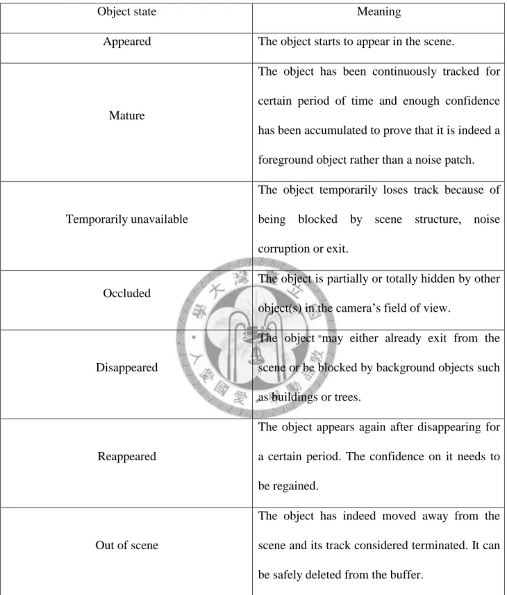
The states of objects in images vary and depend on the relative positions between objects. Lei and Xu provided possible conditions in table 1.2 [31]. When an object appears in camera view for first time, it belongs to the class “Appeared”. In following images if the object is recognized, its state is

“Mature”, we can update its object model. While the object is blocked by background objects, we can’t track it because it is temporarily unavailable in tracking process, so its state will be

“Disappeared”. When it appears again and its previous state is “Disappeared”, its state will be transferred to “Reappeared”. If the object leaves from camera view and we judge that it never return because of its trajectory, its state becomes “Out of scene”. Two conditions are hard to determine, when an object is hidden by other objects, which is the typical case of occlusion, and its state is

“Occluded”. The other case is that an object is corrupted by noise, scene or exit, we can’t identify the object precisely, then its state is “Temporarily unavailable”.

For dynamic scenes the background scene usually changes, it’s necessary to adjust background model to fit the fact. Sample consensus (SACON) is a mechanism of background update [22]. It made use of red, green color values and illumination intensity as standards to extract foreground pixels. Considering the effects of light, if a pixel’s red and green values change dramatically but illumination value doesn’t, this pixel won’t be assigned to a foreground pixel. The background model updates in pixel and blob levels. In pixel level, system creates a counter for each pixel, the counter records how long its corresponding pixel classified as a foreground pixel. When the value of a counter exceeds the threshold value, the pixel will be assigned as a background pixel. In blob level, system also set a counter for each pixel, the counter records how long the pixel as foreground pixel, but in advance the pixel must belong to an object. When the counter is larger than threshold value, the pixel will be updated to be a background pixel, because the object which the pixel belonged to is static for a long time.

Object state Meaning

Appeared The object starts to appear in the scene.

Mature

The object has been continuously tracked for certain period of time and enough confidence has been accumulated to prove that it is indeed a foreground object rather than a noise patch.

Temporarily unavailable

The object temporarily loses track because of being blocked by scene structure, noise corruption or exit.

Occluded

The object is partially or totally hidden by other object(s) in the camera’s field of view.

Disappeared

The object may either already exit from the scene or be blocked by background objects such as buildings or trees.

Reappeared

The object appears again after disappearing for a certain period. The confidence on it needs to be regained.

Out of scene

The object has indeed moved away from the scene and its track considered terminated. It can be safely deleted from the buffer.

Table 1.2︰The number of defined states that an object may enter in a dynamic visual scene.

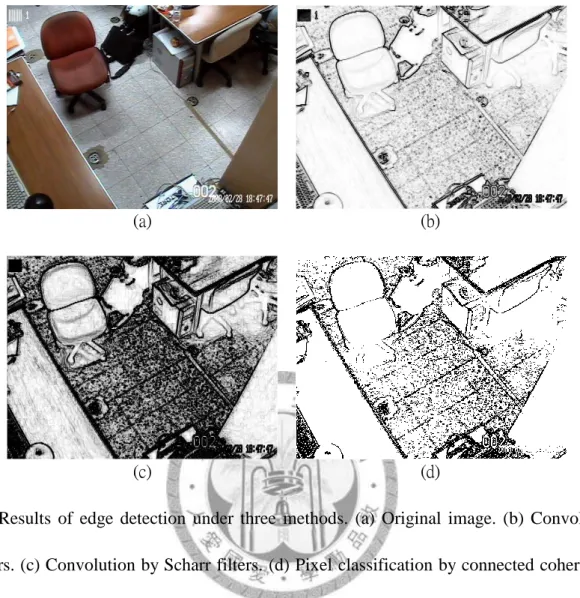
We implemented three concepts mentioned above to analyze an image, the results are displayed in figure 1.2. The original image is figure 1.2a, it’s a monitored view, and we can see desks and chairs within it. We processed the image with Sobel filters and showed the result in figure 1.2b, the settings of the sizes of filters are 3x3 and orientations are vertical, horizontal, and diagonal, total 4 filters. Scharr filters are implemented in figure 1.2c, the settings are identical to Sobel filters. It’s obvious that edges are thicker and darker than figure 1.2b. But many detailed parts are smoother than figure 1.2b. Figure 1.2d is not processed with filters, we took advantage of connected coherence tree algorithm to classify pixels in figure 1.2a. The size of blocks is 3x3 and pixels in white are seeds. This figure is sharper than figure 1.2b but the detailed parts are also not clear comparing to figure 1.2c. Note：In figure 1.2b and 1.2c we assigned pixels’ grayscale intensities according the results of convolutions, but in figure 1.2d the colors of pixels are only white and black because the groups of pixel are only “seed” and “not seed”.

1.4

Thesis Organization

In remaining parts of this thesis we discussed multiple methods proposed by us or other researchers, some are modified to achieve better performance. Finally the results of experiments are showed to validate our system is robust and efficient. Next two sections are important processes in our system, we introduced a background model and two mechanisms to extract foregrounds in chapter 2. We intend to integrate the two mechanisms to eliminate drawbacks of them. Auxiliary parts such as shadow detection and hole filling are introduced later in the section. In chapter 3 there are two filters which can be used to match models and motion objects found in foregrounds. Feature extraction and identification are key points of tracking in the section. chapter 4 and 5 are experiment results and conclusion, respectively. We tested our system with several videos of different scenarios and analyzed results.

(a) (b)

(c) (d)

Fig. 1.3：Results of edge detection under three methods. (a) Original image. (b) Convolution by Sobel filters. (c) Convolution by Scharr filters. (d) Pixel classification by connected coherence tree algorithm.

2 Preprocessing Work

Before beginning tracking motion objects, we must do some preprocessing works to improve the efficiency of tracking. Two important tasks of this are background modeling and deciding the possible foregrounds. Dynamic background model is necessary if background objects are not stationary, especially outdoor scenes. With suitable background model we can extract foregrounds accurately, but the influences of light and shadow will often interfere with our system, we also proposed color-based methods to solve related problems.

2.1 Background Model Construction

The background source can be made from two cases, one is the frames without motion objects, we can call them “real backgrounds” because only stationary objects involved. The foreground will be extracted correctly if using efficient methods, but due to some effects like light, shadow and electro-mechanical problems, background model may deviate away from the reality. There are lots of solutions to this problem, such as building a nearly perfect model or updating model after we receive new frames.

The other case is taking previous frame as the current background model, we do not consider the effects of light if the time interval between two continuous frames is short. But after frame subtraction the foreground may not equal motion object, because the overlay regions of motion object in the two frames won’t present obvious difference, this leads to that only parts of motion objects are regarded as foregrounds. This issue will cause difficulty for object tracking.

Considering the pros and cons of the two cases of background models, we choose the first as our mechanism and develop suitable updating method to do foreground extraction.

To save computing time in real-time environment, we divide background image into blocks with the same size. For every block we compute the mean and standard deviation of intensity of all pixels in it [8]. Then we call the contrast of a block as

) , (

) , j) (

C(i, i j

j i



 

where (i,j) is the position of the block, ( ji, ) the standard deviation, ( ji, ) the mean of intensity. An advantage of dividing images into blocks is reducing the influences of noise pixels, because the importance of a pixel is relatively low in block level.

We also evaluate color and brightness distortion of each block [9]. In background model the brightness distortion of a block of position (i,j) in frame k is

2 2

2

2 2

2 ,

,

)) , (

) , ( ( )) , (

) , ( ( )) , (

) , ( (

) , (

) , ( ) , , ( )

, (

) , ( ) , , ( )

, (

) , ( ) , , (

j i

j i j

i j i j

i j i

j i

j i k j i I j

i

j i k j i I j

i

j i k j i I

B B G

G R

R

R B B

R G G

R R R

k j i











 





















 (2.2)

where_R( ji, ), _G( ji, ) and _B( ji, ) are mean red, green, and blue values of pixels in a block whose position is (i,j) of all background frames, respectively. _R( ji, ), _G( ji, ) and _B( ji, ) are standard deviations of red, green, blue values of pixels in this block of all background frames, respectively. I_R(i,j,k), I_G(i,j,k) and I_B(i,j,k) represent red, green and blue values of the block of background frame no. k. We can find that if a block is brighter than average, its brightness distortion value is high than 1, otherwise the value will be lower than 1 if the block is darker than average. In brief, the value will approximate 1 if the color of block is similar to average no matter the value is greater or lower than 1.

Now we compute color distortion of block in position (i,j),

) . )

, (

) , ( )

, , ( (

, ,

, 2 , ,

,





 

B G R

C C

C k j i C

k j

i

i j

j i k

j i CD I







(2.3)

We can see that _i,j,k is a scale factor of CD_i,j,k. In short, the distortion is similar to the square root of z-score sums.

There are N _i,j,k and CD_i,j,k values in N background frames, with these we can estimate the variation of brightness distortion of block in position (i,j) by computing the root mean square of the distortion,

RMS N a

N

k

k j i j

i j

i









2 ,

, ,

,

) 1 (

) (





N CD CD

RMS b

N

k

k j i j

i j

i







2 , , ,

,

) (

)

(

The two variation values will be factors of threshold to decide foregrounds.

To avoid the influences like light and shadow in individual frame, we take multiple background frames and computed mean contrast values of every block in every frame. It may take much time to do the computation, but this can be finished in advance.

All the information will be compared with current frames for foreground extraction and motion object identification later.

2.2 Foreground Extraction

2.2.1 Method 1

We also compute the values of mean, standard deviation and contrast of all blocks in current frames.

Afterwards, we compare the contrasts of blocks in the same position between background model and current frame. If the difference of contrasts between two blocks exceeds the threshold we set previously (the value will be assigned empirically), the block will be called “foreground block”, otherwise it is a background block.

Drawbacks of the above method would produce include the following. When a pure-colored block (ex. all the colors of pixels in the block are white) changes to another pure-colored block, the standard deviations of them are both zero so that both their contrasts are zero. It means that the difference of contrast is zero that the block wouldn’t identify as a foreground block.

2.2.2 Method 2

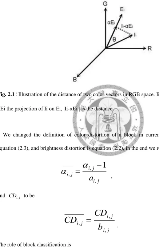
To compensate the problems, another approach from [9] was applied (Huang and Chen proposed a modified version in [19]). We also modified the method from pixel to block level. In figure 2.1, Ei represents the color vector of ith block in background model, its contents include its mean RGB values. And Ii is the same block but from current frame instead. Next, αEi is the projection of Ii on Ei, we compute the length of difference between Ii and αEi, that is, | Ii-αEi |, this will be an index for us to estimate whether a block is foreground block or not (| Ii-αEi | is called the color distortion of i in [9]). The decision is simple, if the value is greater than threshold, the block will be a foreground block.

If a color vector is part of the other vector or vice versa, it indicates the distance | Ii-αEi | is 0, with above definition the block won’t be a foreground block. For example, v₁ = (50,50,50) and v₂ = (200,200,200). In RGB color space v1 is a color nearly gray, and v2 is nearly white. It reveals a controversy that the two colors are similar or not, and we choose to comply with the original

definition. There are some disadvantages of this mechanism discovered in experiments, we modified the algorithm to reduce failures in foreground extraction.

Fig. 2.1：Illustration of the distance of two color vectors in RGB space. Ii and Ei are the two vectors, αEi the projection of Ii on Ei, |Ii-αEi | is the distance.

We changed the definition of color distortion of a block in current frame from | Ii-αEi | to equation (2.3), and brightness distortion is equation (2.2), in the end we rescale _i,j to be

j i j i j

i

a

, ,

 1

 



j i

j i j

i

b

CD CD

, ,

,



. (2.7)

The rule of block classification is

, :

and :

:

2

1 ,

,

, ,

 



 











otherwise H

T T

B

T or

T CD

F

j i j

i

j i CD

j i













(2.8)

where F is abbreviation of foreground block, T_CD and T are thresholds for _ CD_i,j and _i,j, respectively. The two conditions are decisions that a block is either discriminative in color or brightness. B represents background block,

1

T and

2

T are upper and lower bound of _i,j, that is, a block belongs to background if its _i,j locates between

1

T and

2

T . H is the group of other situations.

After identifying all foreground blocks in current frame, we merge these blocks to “foreground regions”. A foreground region is a connected component of foreground blocks. The definition of connection is that if two foreground blocks are 8-neighbors, they are connected, otherwise they are not. Because of the effect of noise, we set a threshold for foreground regions, if the size of a region didn’t exceed the threshold, the region will be treated as noise instead of foreground, even if exactly the region contains motion objects. To express the foreground region easily, the region will be represented by a rectangle whose length and width are multiples of length and width of a block, respectively. So in a foreground region there are both foreground and background blocks, even the later locate in a region, they won’t be analyzed in following processes.

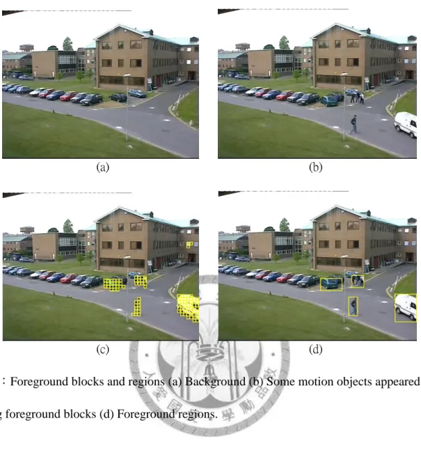
Figure 2.2 showed the performance of foreground extraction, figure 2.2a is one of background frame, which is similar to background model. We can see some people and cars in figure 2.2b, which represent motion objects. The blocks in figure 2.2c are foreground blocks, they cover these objects and parts of a window of the building in rear of motion objects. We combined these blocks in figure 2.2d, four objects are surrounded by large blocks, but because of the threshold of size, the window in top-right side of the image is ignored.

(a) (b)

(c) (d)

Fig. 2.2：Foreground blocks and regions (a) Background (b) Some motion objects appeared (c) Drawing foreground blocks (d) Foreground regions.

Sudden change of light is another problem of background subtraction, in indoor scene the light source is usually from electronic lights, which can’t always offer rays with stable intensity or sometimes are influenced by objects near them. In outdoor scene, the light source is usually sunlight, whose intensity can be affected by cloud and change with time. In a cloudy day, we can figure out there is not enough light source to take sharp pictures.

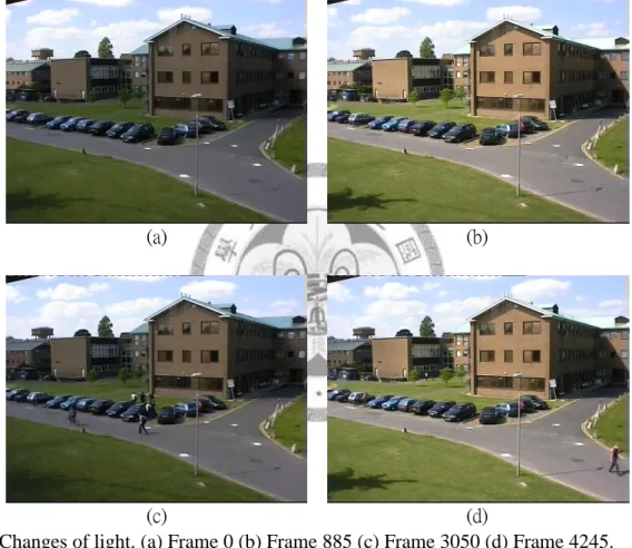
Some examples of light switch are displayed in figure 2.3, the sources of images are from PETS2001 dataset 3, we snapshot some frames of the video. Figure 2.3a is the first frame in the video, the background is almost identical to figure 2.2. A apparent light change happened in figure 2.3b, the intensity of light source increased, it’s believed that the reason is moving cloud. In figure

2.3c and figure 2.4d there are also obvious light changes, the former is darker than figure 2.3b and the later is similar to figure 2.3b. It’s interesting that in the video with length about 5 minutes, there are various light switches between frames. Tracking process in the video will be a great challenge duo to the various intensities of light source. With the kind of video we have to build background model carefully to adapt light problems.

(a) (b)

(c) (d)

Fig. 2.3：Changes of light. (a) Frame 0 (b) Frame 885 (c) Frame 3050 (d) Frame 4245.

2.3 Background Model Updating

In previous section we discussed the problems of background modeling. To match the current background we have to update the model. Something may join the background after we begin tracking, we can find that blocks corresponding to these things always recognized as foreground

blocks if we don’t update the original background model, but in fact they have became parts of backgrounds.

We create a counter for all blocks [10]. When a block is recognized as a foreground block, the counter of this block will increment, otherwise subtract. If the counter exceeds the threshold, it means that the frequency of the block recognized as a foreground block for a period of time is large enough for us to update the block in background model. For example, if the threshold is set to 50, a block must to be assigned to a foreground block at least 51 frames in 100 consecutive frames, or 101 frames in past 200 frames. If we update a block in background model, the contrast and mean intensity of block in the model will be replaced by the mean contrast and mean intensity of all foreground blocks with the same position in previous frames, respectively.

3 Object Recognition and Tracking

From previous work we acquire foreground regions, which are possible motion objects. Here we propose two filters (or two color-based techniques) to create object models and identification objects.

Motion objects in camera view often change their appearance, when a man walks to camera, the region he belongs to in frames will get larger, this is the problem of scale. Every object may change his direction while moving, this is the problem of orientation. Finally, a terrible situation is occlusion, which happens when objects covered by backgrounds or other objects, only parts of this object emerge, we can’t discriminate it by global information collected before.

First, we compare the similarity of color distribution of every pair, one selected from foreground regions (blobs) and the other from motion object models. If a pair is similar by our definition, the comparison of detailed information of all foreground blocks and motion object model will be carried out in second step.

3.1 Global Color Similarity Comparison

In the beginning we check the similarity of foreground regions and motion object models by color histograms. The histogram is composed of all the color intensity of pixels in foreground regions instead of mean color intensity of every block.

The color intensity will be divided into bins, every intensity value belongs to only one bin. From [11], considering the spatial relation, we assign weights to a pixel by its distance to central pixel in the foreground region, the possibility of a intensity value assigned to a bin u is



 ⁿ

i

i

i x

x k C Pu

1

u]

- ) [b(

|)

(|



Kronecker delta function, b(x_i) the bin x_i belonged to. Finally C normalizes P(u) in the range of 0 and 1,



 _n

i

xi

k C

0

|) (|

1

, (3.2)

Then, from experience we know that the scales of objects change frequently, using |x as _i| parameter of weighting function is not proper. The parameter would be changed to the relative (normalized) distance between a pixel and the central point of foreground region. Then (3.1) will be adjusted as



 ⁿ

i

i

h k x C Pu

1

i)-u]

[b(x

|)

(|



where h is the scale of foreground region, a practical definition is the maximum of all pixels in the region to central point, it is, the distance of central point to any corner of the region. And the distance is estimated by Euclidean distance.

Finally the color similarity of foreground regions and motion object models can be evaluated by Bhattacharyya coefficient,





 ⁿ

1 u

) ( [p(y)q]

(y)





note y is the central point of foreground region, p the foreground region, q the object model.

Because the possibility of each bin is between 0 and 1, and we have to normalize the two distributions of possibilities to guarantee that









u u n

u

u

and q

p

1 1

1

1

which indicates for any bin u, the product of p and _u q will locate in the range of 0 and 1, and _u the square root of their product would occur in the same range. For two identical distributions, the

Bhattacharyya coefficient of them is 1. For two similar distributions, their Bhattacharyya coefficient will be close to 1. In [26], Nummiaro at al. set the threshold for the coefficient to decide two objects are similar to be





 [ p ( y ) q ]   2

where  and  are mean and standard deviation of Bhattacharyya coefficients computed in history records. The threshold value indicates the two objects have least 97.5% confidence that they are similar in global color distributions. But we don’t set the threshold that high, the value of threshold





 [ p ( y ) q ]   2

When the similarity of a pair exceeds the threshold, it represents that the pair passed the first filter, in next step we will verify if the region matches to the model in terms of detailed information. If not, there are three possible cases [12]:

Case 1：Occlusion happens, that is, more that one motion objects overlaid in the frame, foreground region contains these objects implies the color histogram is the mixture of them. Because this filter can only analyze global information of objects, we just assume the situation (there are multiple motion objects in a region) happens but we can’t confirm it using the filter.

The other filter will identify the situation because it compares local information.

Case 2：Motion objects changes their appearances or are occluded by background objects. For example, a man puts on a jacket, turns his head, or is sheltered by a desk. We can solve the problem by assigning an active position for every motion object model. If the distance of a foreground region and an object model is short, it’s very possible that the region matched the model. Every time we meet the situation, the threshold of similarity (Bhattacharyya

coefficient) will subtract to avoid this case. Note that tolerance degree increases may result in recognition failures.

Case 3：New object emerges, we can’t let the object match to any models through the two filters, and we should create a new model for this object.

Here a model contains the color distribution of the object and the last position it occurred. If an object hasn’t appeared for a period of time, the model corresponding to it would be deleted because we must save memory space and computing time. Like background model, we will update motion object models to become closer to reality when an object matches to a model,

u u

u

p q

q    ( 1   )

3.2 Detailed Information Comparison

When a pair of object and model passed first filter, it means that the global color histograms of the two objects is similar, here we check the information in all blocks within them. The contrast context histogram can be used as a tool to decide the similarity of two points in different images [13]. When an image changes on scales or orientation, this method can find similar even identical pairs of pixels in two images. The features they extracted from a pixel are color histograms of pixels around it.

First classifying these pixels to groups in terms of their distances and orientations to this pixel Pc (figure 3.1a), for every group computing the mean intensity values higher and lower than Pc. In the end these values will be integrated to form a feature vector of this pixel. Comparing every feature vector of pixels in different images will acquire similar pixel pairs. For the problem of scales, adjusting the size (number of pixels) of groups is an efficient approach but it needs empirical rule to

decide the size. To solve the orientation problem, shifting feature vectors will be a good idea because it is just like to rotate the image to fit the other image.

Whatever the measures we use, it takes much time to compare objects in pixel level. Here we use blocks instead to accelerate computation, so we modified the original algorithm from pixel to block level.

(a) (b)

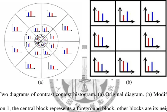
Fig. 3.1：Two diagrams of contrast context histogram. (a) Original diagram. (b) Modified diagram.

In application 1, the central block represents a foreground block, other blocks are its neighbor blocks.

We computed two values for each neighbor block. In application 2, a foreground block will be divided into 9 sub-blocks, we also computed 2 values for 8 outer sub-blocks.

A foreground region is composed of foreground blocks, for every neighbor block of every block, we compute the mean intensity of pixels in neighbor block higher than the block and lower than it.

That is, for a block B and its neighbor B_i, the mean intensity value of pixels in B_i higher than B is





 

i

i i

B B

B I x I and B x x B I

H i

#

)}

( ) (

| ) ( ) {

( , (3.9)

and the lower case is



 ^{ }





i

i i

B

B

B I x I and B x x B I

H

#

)}

( ) (

| ) ( ) {

(

where I(x) is the color intensity of pixel x, I(B_i) is the mean color intensity of B_i, #B_i+ is the number of pixels whose color intensities are greater than I(Bi). #Bi- is the number of pixels belong to the lower case.

Then we get two values from each neighbors (figure 3.1b), 16 values totally (8-neighbor). We made a feature vector for each foreground block, the vector involved 16 values about neighbor blocks and mean red, green, and blue values of this block. It can represent by

)}

( ), ( ), ( , , ,...,

, { )

(B H 1 H 1 H 8 H 8 r B g B b B

CCH  _{B B B B} , (3.10)

where r(B), g(B) and b(B) are mean red, green and blue values of block B.

Comparing all the foreground blocks of region and model by theirs feature vectors, we can evaluate the similarity of detail information between an object and an object model. Considering object orientation, we “rotate” these 16 values about neighbor blocks in feature vector to meet the case that object changes its direction. A neighbor block can rotate 7 times to locate in other place in figure 3.1, a feature vector can also exchange its contents 7 times when comparing in the same meaning.

The clockwise rotation procedure is shown in figure 3.2, the block no.5 is the block we want to extract features, other blocks are its neighbor blocks in figure 3.2a. After first rotation the arrangement of these blocks are shown in figure 3.2b, each block shift to its neighborhood except the block no.5. We can see the final result after 7 rotations in figure 3.2c.

The neighbor blocks of boundary blocks changed when objects moved. Some neighbors are composed of backgrounds, it means the feature vectors we compute above are not adequate for boundary blocks. In case of errors, we compute features inside a block too. To keep the same form, we divided a block into nine sub-blocks of identical size, the interior sub-block (in figure 3.2a, it’s

the block no.5) will be ignored. Two same values (mean intensity values of pixels greater and lower than interior sub-block) will be computed from every exterior sub-block (in figure 3.2a, they are blocks except block no.5), joining with mean red, green, blue values of the block, total 19 value as feature vector inside the block.

(a) (b) (c)

Fig 3.2：Clockwise rotation results of neighbor blocks. (a) Before rotation. (b) After first rotation. (c) After last (7th) rotation.

The detailed model includes the information of neighbor blocks, mean color intensity, its area in the frame, and latest time when blocks occurred. The feature vectors of an object model are collected from appearances of the object in previous frames. Old feature vectors will be replaced by new ones. Area and timestamp can help a lot, objects can’t enlarge or shrink in a short time, and their positions can’t vary dramatically in consecutive frames. With auxiliary information we could identify and track objects more accurately. A model will be deleted if it hasn’t appeared for a long time.

Some examples of detailed object information recognition are displayed in figure 3.3. The scenario of this video (provided by Kun-Chen Tsai, Institute for Information Industry [33]) is a man walked from left to right side, and fell down several seconds later, finally he stood up and left. In

figure 3.3a he appeared, we build and update his model in current and following frames. In figure 3.3b to figure 3.3d he expressed different poses, we analyze his detailed features. Little blocks are drawn as long as the features in the blocks match to his detailed model, we catch about 70 to 80 percentages of his body in these three frames.

(a) (b)

(c) (d)

Fig. 3.3：Recognition of detailed object models. (a) Frame 120 (b) Frame 185 (c) Frame 205 (d) Frame 230

3.3 Occlusion Detection

A tough problem of tracking is occlusion. We can predict interaction of motion objects by information of objects. Positions and velocities of objects are usual cues for us to predict possible situation in following frames. “Occlusion grid” is a simple but efficient method to record and predict positions of objects [32]. The locations of objects will be recorded in the grid, an example is figure

3.4. With the grid, and we modified two filters introduced in section 3.1 and 3.2 to detect two cases of occlusion. The first case is a foreground region contains more than one motion objects, and the other case is a motion object covered by backgrounds. When a foreground region couldn’t match to any models by filter 1, we compare the foreground blocks and detailed features of all models, according to the result we take different actions. If no models exist in the region, the region represents a new object, and we create a new model for it. If just one model is recognized, it means that the object was covered by background or it changed its appearance. Otherwise, if more than one models recognized, occlusion of some motion objects happened. Note that when occlusion took place, we didn’t update the detailed model of identified objects because we assumed these features are biased.

Fig 3.4：An example of occlusion grid. The numbers in sub-grids are object IDs. We can see occupied locations of objects in images from the grid. In the example object 1 and 2 interacted because there are sub-grids which belong to them.

In figure 3.5, there are 4 examples of occlusions. In figure 3.5a, a man is covered by a desk, lower parts of his legs are hidden, it is an example of objects were covered by backgrounds. In figure 3.5b a man was covered by the other man, we can only recognize the rear man by his head and upper body. We can see a van located in front of three men in figure 3.5c, most parts of the left two men hid because of the van. And a black car sheltered the white van in figure 3.5d.

(a) (b)

(c) (d)

Fig 3.5：Occlusion examples. (a) Object was covered by background. (b)(c)(d) Objects were covered by other objects, which are pedestrians or vehicles.

We also show some examples of results of occlusion solution in the video of first view of PETS2001 dataset 1, which included lots of cases of occlusion that objects covered other objects. In figure 3.6a, two vehicles have been tracked and modeled and are represented by two blocks in green and blue. The van was going forward along the road and the other car pulled up in a parking space.

The pedestrians in right side of the frame didn’t be tracked because their size is lower than the threshold for object size. From figure 3.6b to figure 3.6d, occlusion cases happened as the two vehicles existed in the same foreground region, the little blocks in green and blue represent they belong to which object model after analyzing the detailed models. Here the global color feature of these foreground regions are useless, we have to compare detailed features in regions to identify the occlusion cases.

(a) (b)

(b) (d)

Fig. 3.6：Results of occlusion solution by detailed models part 1. (a) Frame 775 (b) Frame 815 (c) Frame 825 (d) Frame 870

The other occlusion case that motion objects are covered by backgrounds is shown in figure 3.7.

The source of this video is PETS2001 dataset 2, it’s the first view of two. We recognized and tracked the whole body of target in figure 3.7a and 3.7b, of course we got more information

concerning the object to update object model. The target was occluded in figure 3.7c and 3.7d, the two frames are original (raw data) in the video. Some parts of this car were covered by a tree, we must identify this car by detailed features. The analytic results of the two frames are shown in figure 3.7e and 3.7f, little blocks means they matched to the detailed model.

(a) (b)

(c) (d)

(e) (f)

Fig. 3.7：Results of occlusion solution by detailed models part 2. (a) Frame 340 (b) Frame 355 (c) Frame 1145 (d) Frame 1180 (e)(f) The results of occlusion solution of (c) and (d), respectively.

With the discussion in the chapter, we summary all conditions based on a foreground region pass the two filters or not in table 3.1.

Pass filter 1? Pass filter 2? Results

Yes Yes Matching to a model.

Yes No

Case 1：Matching to a wrong model.

Case 2：The region includes more than one object.

No Yes

Case 1：Matching to a model but the object is occluded.

Case 2：The region includes more than one object.

No No New object

Table 3.1：Four conditions of foreground region.