J.3 Floating Point J-13
J.4 Floating-Point Multiplication J-17
J.5 Floating-Point Addition J-21
J.6 Division and Remainder J-27
J.7 More on Floating-Point Arithmetic J-32
J.8 Speeding Up Integer Addition J-37
J.9 Speeding Up Integer Multiplication and Division J-44
J.10 Putting It All Together J-58
J.11 Fallacies and Pitfalls J-62
J.12 Historical Perspective and References J-62
Exercises J-68
J
Computer Arithmetic 1
by David Goldberg
Xerox Palo Alto Research Center
The Fast drives out the Slow even if the Fast is wrong.
W. Kahan
Although computer arithmetic is sometimes viewed as a specialized part of CPU design, it is a very important part. This was brought home for Intel in 1994 when their Pentium chip was discovered to have a bug in the divide algorithm. This floating-point flaw resulted in a flurry of bad publicity for Intel and also cost them a lot of money. Intel took a $300 million write-off to cover the cost of replacing the buggy chips.
In this appendix, we will study some basic floating-point algorithms, includ- ing the division algorithm used on the Pentium. Although a tremendous variety of algorithms have been proposed for use in floating-point accelerators, actual implementations are usually based on refinements and variations of the few basic algorithms presented here. In addition to choosing algorithms for addition, sub- traction, multiplication, and division, the computer architect must make other choices. What precisions should be implemented? How should exceptions be handled? This appendix will give you the background for making these and other decisions.
Our discussion of floating point will focus almost exclusively on the IEEE floating-point standard (IEEE 754) because of its rapidly increasing acceptance.
Although floating-point arithmetic involves manipulating exponents and shifting fractions, the bulk of the time in floating-point operations is spent operating on fractions using integer algorithms (but not necessarily sharing the hardware that implements integer instructions). Thus, after our discussion of floating point, we will take a more detailed look at integer algorithms.
Some good references on computer arithmetic, in order from least to most detailed, are Chapter 3 of Patterson and Hennessy [2009]; Chapter 7 of Ham- acher, Vranesic, and Zaky [1984]; Gosling [1980]; and Scott [1985].
Readers who have studied computer arithmetic before will find most of this sec- tion to be review.
Ripple-Carry Addition
Adders are usually implemented by combining multiple copies of simple com- ponents. The natural components for addition are half adders and full adders.
The half adder takes two bits a and b as input and produces a sum bit s and a carry bit cout as output. Mathematically, s = (a + b) mod 2, and cout = ⎣(a + b)/
2⎦, where ⎣ ⎦ is the floor function. As logic equations, s = ab + ab and cout = ab, where ab means a ∧ b and a + b means a ∨ b. The half adder is also called a (2,2) adder, since it takes two inputs and produces two outputs. The full adder
J.1 Introduction
J.2 Basic Techniques of Integer Arithmetic
J.2 Basic Techniques of Integer Arithmetic ■ J-3
is a (3,2) adder and is defined by s = (a + b + c) mod 2, cout = ⎣(a + b + c)/2⎦, or the logic equations
J.2.1 s = ab c + abc + abc + abc J.2.2 cout = ab + ac + bc
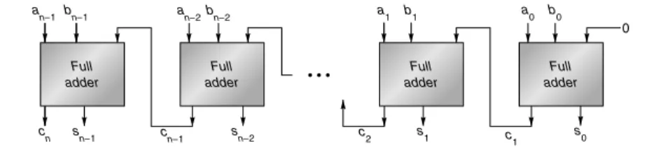
The principal problem in constructing an adder for n-bit numbers out of smaller pieces is propagating the carries from one piece to the next. The most obvi- ous way to solve this is with a ripple-carry adder, consisting of n full adders, as illustrated in Figure J.1. (In the figures in this appendix, the least-significant bit is always on the right.) The inputs to the adder are an–1an–2 ⋅ ⋅ ⋅ a0 and bn–1bn–2 ⋅ ⋅ ⋅ b0, where an–1an–2 ⋅ ⋅ ⋅ a0 represents the number an–1 2n–1 + an–2 2n–2 + ⋅ ⋅ ⋅ + a0. The ci+1 output of the ith adder is fed into the ci+1 input of the next adder (the (i + 1)-th adder) with the lower-order carry-in c0 set to 0. Since the low-order carry-in is wired to 0, the low-order adder could be a half adder. Later, however, we will see that setting the low-order carry-in bit to 1 is useful for performing subtraction.
In general, the time a circuit takes to produce an output is proportional to the maximum number of logic levels through which a signal travels. However, deter- mining the exact relationship between logic levels and timings is highly technology dependent. Therefore, when comparing adders we will simply compare the number of logic levels in each one. How many levels are there for a ripple-carry adder? It takes two levels to compute c1 from a0 and b0. Then it takes two more levels to compute c2 from c1, a1, b1, and so on, up to cn. So, there are a total of 2n levels.
Typical values of n are 32 for integer arithmetic and 53 for double-precision float- ing point. The ripple-carry adder is the slowest adder, but also the cheapest. It can be built with only n simple cells, connected in a simple, regular way.
Because the ripple-carry adder is relatively slow compared with the designs discussed in Section J.8, you might wonder why it is used at all. In technologies like CMOS, even though ripple adders take time O(n), the constant factor is very small. In such cases short ripple adders are often used as building blocks in larger adders.
Figure J.1 Ripple-carry adder, consisting of n full adders. The carry-out of one full adder is connected to the carry-in of the adder for the next most-significant bit. The carries ripple from the least-significant bit (on the right) to the most-significant bit (on the left).
bn–1 an–1
sn–1
Full adder
cn–1 s
c n–2 n
an–2b
n–2
Full adder
b1 a1
s1
Full adder
s0 a0 b0
Full adder
c2 c1
0
Radix-2 Multiplication and Division
The simplest multiplier computes the product of two unsigned numbers, one bit at a time, as illustrated in Figure J.2(a). The numbers to be multiplied are an–1an–2
⋅ ⋅ ⋅ a0 and bn–1bn–2 ⋅ ⋅ ⋅ b0, and they are placed in registers A and B, respectively.
Register P is initially 0. Each multiply step has two parts:
Multiply Step (i) If the least-significant bit of A is 1, then register B, containing bn–1bn–2 ⋅ ⋅ ⋅ b0, is added to P; otherwise, 00 ⋅ ⋅ ⋅ 00 is added to P. The sum is placed back into P.
(ii) Registers P and A are shifted right, with the carry-out of the sum being moved into the high-order bit of P, the low-order bit of P being moved into register A, and the rightmost bit of A, which is not used in the rest of the algorithm, being shifted out.
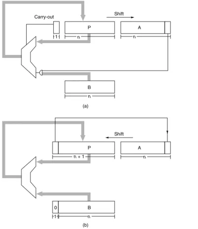
Figure J.2 Block diagram of (a) multiplier and (b) divider for n-bit unsigned integers.
Each multiplication step consists of adding the contents of P to either B or 0 (depend- ing on the low-order bit of A), replacing P with the sum, and then shifting both P and A one bit right. Each division step involves first shifting P and A one bit left, subtracting B from P, and, if the difference is nonnegative, putting it into P. If the difference is nonnegative, the low-order bit of A is set to 1.
Carry-out
P A
n
n
n Shift
P
B 0
A n + 1
n 1
n Shift (a)
(b) 1
B
J.2 Basic Techniques of Integer Arithmetic ■ J-5
After n steps, the product appears in registers P and A, with A holding the lower-order bits.
The simplest divider also operates on unsigned numbers and produces the quotient bits one at a time. A hardware divider is shown in Figure J.2(b). To com- pute a/b, put a in the A register, b in the B register, and 0 in the P register and then perform n divide steps. Each divide step consists of four parts:
Divide Step (i) Shift the register pair (P,A) one bit left.
(ii) Subtract the content of register B (which is bn–1bn–2 ⋅ ⋅ ⋅ b0) from register P, putting the result back into P.
(iii) If the result of step 2 is negative, set the low-order bit of A to 0, otherwise to 1.
(iv) If the result of step 2 is negative, restore the old value of P by adding the contents of register B back into P.
After repeating this process n times, the A register will contain the quotient, and the P register will contain the remainder. This algorithm is the binary ver- sion of the paper-and-pencil method; a numerical example is illustrated in
Figure J.3(a).
Notice that the two block diagrams in Figure J.2 are very similar. The main difference is that the register pair (P,A) shifts right when multiplying and left when dividing. By allowing these registers to shift bidirectionally, the same hard- ware can be shared between multiplication and division.
The division algorithm illustrated in Figure J.3(a) is called restoring, because if subtraction by b yields a negative result, the P register is restored by adding b back in. The restoring algorithm has a variant that skips the restoring step and instead works with the resulting negative numbers. Each step of this nonrestoring algorithm has three parts:
Nonrestoring If P is negative,
Divide Step (i-a) Shift the register pair (P,A) one bit left.
(ii-a) Add the contents of register B to P.
Else,
(i-b) Shift the register pair (P,A) one bit left.
(ii-b) Subtract the contents of register B from P.
(iii) If P is negative, set the low-order bit of A to 0, otherwise set it to 1.
After repeating this n times, the quotient is in A. If P is nonnegative, it is the remainder. Otherwise, it needs to be restored (i.e., add b), and then it will be the remainder. A numerical example is given in Figure J.3(b). Since steps (i-a) and (i-b) are the same, you might be tempted to perform this common step first, and then test the sign of P. That doesn’t work, since the sign bit can be lost when shifting.
The explanation for why the nonrestoring algorithm works is this. Let rk be the contents of the (P,A) register pair at step k, ignoring the quotient bits (which are simply sharing the unused bits of register A). In Figure J.3(a), initially A con- tains 14, so r0 = 14. At the end of the first step, r1 = 28, and so on. In the restoring Figure J.3 Numerical example of (a) restoring division and (b) nonrestoring division.
00000 00001 –00011 –00010 00001 00011 –00011 00000 00001 –00011 –00010 00001 00010 –00011 –00001 00010
1110 110
1100 1100 100
1001 001
0010 0010 010
0100 0100
Divide 14 = 1110
2 by 3 = 11
2. B always contains 0011
2. step 1(i): shift.
step 1(ii): subtract.
step 1(iii): result is negative, set quotient bit to 0.
step 1(iv): restore.
step 2(i): shift.
step 2(ii): subtract.
P A
step 2(iii): result is nonnegative, set quotient bit to 1.
step 3(i): shift.
step 3(ii): subtract.
step 3(iii): result is negative, set quotient bit to 0.
step 3(iv): restore.
step 4(i): shift.
step 4(ii): subtract.
step 4(iii): result is negative, set quotient bit to 0.
step 4(iv): restore. The quotient is 01002 and the remainder is 000102.
00000 00001 +11101 11110 11101 +00011 00000 00001 +11101 11110 11100 +00011 11111 +00011 00010
1110 110
1100 100
1001 001
0010 010
0100
Divide 14 = 11102 by 3 = 112. B always contains 00112. step 1(i-b): shift.
step 1(ii-b): subtract b (add two’s complement).
step 1(iii): P is negative, so set quotient bit to 0.
step 2(i-a): shift.
step 2(ii-a): add b.
step 2(iii): P is nonnegative, so set quotient bit to 1.
step 3(i-b): shift.
step 3(ii-b): subtract b.
step 3(iii): P is negative, so set quotient bit to 0.
step 4(i-a): shift.
step 4(ii-a): add b.
step 4(iii): P is negative, so set quotient bit to 0.
Remainder is negative, so do final restore step.
The quotient is 01002 and the remainder is 000102. (b)
(a)
J.2 Basic Techniques of Integer Arithmetic ■ J-7
algorithm, part (i) computes 2rk and then part (ii) 2rk− 2nb (2nb since b is sub- tracted from the left half). If 2rk − 2nb ≥ 0, both algorithms end the step with identical values in (P,A). If 2rk− 2nb < 0, then the restoring algorithm restores this to 2rk, and the next step begins by computing rres = 2(2rk) − 2nb. In the non- restoring algorithm, 2rk− 2nb is kept as a negative number, and in the next step rnonres = 2(2rk− 2nb) + 2nb = 4rk− 2nb = rres. Thus (P,A) has the same bits in both algorithms.
If a and b are unsigned n-bit numbers, hence in the range 0 ≤ a,b ≤ 2n− 1, then the multiplier in Figure J.2 will work if register P is n bits long. However, for division, P must be extended to n + 1 bits in order to detect the sign of P. Thus the adder must also have n + 1 bits.
Why would anyone implement restoring division, which uses the same hard- ware as nonrestoring division (the control is slightly different) but involves an extra addition? In fact, the usual implementation for restoring division doesn’t actually perform an add in step (iv). Rather, the sign resulting from the sub- traction is tested at the output of the adder, and only if the sum is nonnegative is it loaded back into the P register.
As a final point, before beginning to divide, the hardware must check to see whether the divisor is 0.
Signed Numbers
There are four methods commonly used to represent signed n-bit numbers: sign magnitude, two’s complement, one’s complement, and biased. In the sign magni- tude system, the high-order bit is the sign bit, and the low-order n − 1 bits are the magnitude of the number. In the two’s complement system, a number and its neg- ative add up to 2n. In one’s complement, the negative of a number is obtained by complementing each bit (or, alternatively, the number and its negative add up to 2n − 1). In each of these three systems, nonnegative numbers are represented in the usual way. In a biased system, nonnegative numbers do not have their usual representation. Instead, all numbers are represented by first adding them to the bias and then encoding this sum as an ordinary unsigned number. Thus, a nega- tive number k can be encoded as long as k + bias ≥ 0. A typical value for the bias is 2n–1.
Example Using 4-bit numbers (n = 4), if k = 3 (or in binary, k = 00112), how is −k expressed in each of these formats?
Answer In signed magnitude, the leftmost bit in k = 00112 is the sign bit, so flip it to 1: −k is represented by 10112. In two’s complement, k + 11012 = 2n = 16. So −k is rep- resented by 11012. In one’s complement, the bits of k = 00112 are flipped, so −k is represented by 11002. For a biased system, assuming a bias of 2n−1 = 8, k is represented by k + bias = 10112, and −k by −k + bias = 01012.
The most widely used system for representing integers, two’s complement, is the system we will use here. One reason for the popularity of two’s complement is that it makes signed addition easy: Simply discard the carry-out from the high- order bit. To add 5 + −2, for example, add 01012 and 11102 to obtain 00112, resulting in the correct value of 3. A useful formula for the value of a two’s com- plement number an–1an–2 ⋅ ⋅ ⋅ a1a0 is
J.2.3 −an–12n–1 + an–22n–2 + ⋅ ⋅ ⋅ + a121 + a0
As an illustration of this formula, the value of 11012 as a 4-bit two’s complement number is −1⋅23 + 1⋅22 + 0⋅21 + 1⋅20 = −8 + 4 + 1 = −3, confirming the result of the example above.
Overflow occurs when the result of the operation does not fit in the represen- tation being used. For example, if unsigned numbers are being represented using 4 bits, then 6 = 01102 and 11 = 10112. Their sum (17) overflows because its binary equivalent (100012) doesn’t fit into 4 bits. For unsigned numbers, detect- ing overflow is easy; it occurs exactly when there is a carry-out of the most- significant bit. For two’s complement, things are trickier: Overflow occurs exactly when the carry into the high-order bit is different from the (to be dis- carded) carry-out of the high-order bit. In the example of 5 + −2 above, a 1 is car- ried both into and out of the leftmost bit, avoiding overflow.
Negating a two’s complement number involves complementing each bit and then adding 1. For instance, to negate 00112, complement it to get 11002 and then add 1 to get 11012. Thus, to implement a − b using an adder, simply feed a and b (where b is the number obtained by complementing each bit of b) into the adder and set the low-order, carry-in bit to 1. This explains why the rightmost adder in Figure J.1 is a full adder.
Multiplying two’s complement numbers is not quite as simple as adding them. The obvious approach is to convert both operands to be nonnegative, do an unsigned multiplication, and then (if the original operands were of opposite signs) negate the result. Although this is conceptually simple, it requires extra time and hardware. Here is a better approach: Suppose that we are multiplying a times b using the hardware shown in Figure J.2(a). Register A is loaded with the number a; B is loaded with b. Since the content of register B is always b, we will use B and b interchangeably. If B is potentially negative but A is nonnegative, the only change needed to convert the unsigned multiplication algorithm into a two’s complement one is to ensure that when P is shifted, it is shifted arithmetically;
that is, the bit shifted into the high-order bit of P should be the sign bit of P (rather than the carry-out from the addition). Note that our n-bit-wide adder will now be adding n-bit two’s complement numbers between −2n–1 and 2n–1 − 1.
Next, suppose a is negative. The method for handling this case is called Booth recoding. Booth recoding is a very basic technique in computer arithmetic and will play a key role in Section J.9. The algorithm on page J-4 computes a × b by examining the bits of a from least significant to most significant. For example, if a = 7 = 01112, then step (i) will successively add B, add B, add B, and add 0.
Booth recoding “recodes” the number 7 as 8 − 1 = 10002 − 00012 = 1001, where
J.2 Basic Techniques of Integer Arithmetic ■ J-9
1 represents −1. This gives an alternative way to compute a × b, namely, succes- sively subtract B, add 0, add 0, and add B. This is more complicated than the unsigned algorithm on page J-4, since it uses both addition and subtraction. The advantage shows up for negative values of a. With the proper recoding, we can treat a as though it were unsigned. For example, take a = −4 = 11002. Think of 11002 as the unsigned number 12, and recode it as 12 = 16 − 4 = 100002− 01002
= 10100. If the multiplication algorithm is only iterated n times (n = 4 in this case), the high-order digit is ignored, and we end up subtracting 01002 = 4 times the multiplier—exactly the right answer. This suggests that multiplying using a recoded form of a will work equally well for both positive and negative numbers.
And, indeed, to deal with negative values of a, all that is required is to sometimes subtract b from P, instead of adding either b or 0 to P. Here are the precise rules:
If the initial content of A is an–1 ⋅ ⋅ ⋅ a0, then at the ith multiply step the low-order bit of register A is ai, and step (i) in the multiplication algorithm becomes:
I. If ai = 0 and ai–1 = 0, then add 0 to P.
II. If ai = 0 and ai–1 = 1, then add B to P.
III. If ai = 1 and ai–1 = 0, then subtract B from P.
IV. If ai = 1 and ai–1 = 1, then add 0 to P.
For the first step, when i = 0, take ai–1 to be 0.
Example When multiplying −6 times −5, what is the sequence of values in the (P,A) register pair?
Answer See Figure J.4.
Figure J.4 Numerical example of Booth recoding. Multiplication of a = –6 by b = –5 to get 30.
0000 0000 0000 + 0101 0101 0010 + 1011 1101 1110 + 0101 0011 0001
1010 1010 0101
0101 1010
1010 1101
1101 1110
Put –6 = 10102 into A, –5 = 10112 into B.
step 1(i): a0 = a–1 = 0, so from rule I add 0.
step 1(ii): shift.
step 2(i): a1 = 1, a0 = 0. Rule III says subtract b (or add –b = –10112 = 01012).
step 2(ii): shift.
step 3(i): a
2 = 0, a
1 = 1. Rule II says add b (1011).
step 3(ii): shift. (Arithmetic shift—load 1 into leftmost bit.) step 4(i): a3 = 1, a2 = 0. Rule III says subtract b.
step 4(ii): shift. Final result is 000111102 = 30.
P A
The four prior cases can be restated as saying that in the ith step you should add (ai–1 − ai)B to P. With this observation, it is easy to verify that these rules work, because the result of all the additions is
Using Equation J.2.3 (page J-8) together with a−1 = 0, the right-hand side is seen to be the value of b × a as a two’s complement number.
The simplest way to implement the rules for Booth recoding is to extend the A register one bit to the right so that this new bit will contain ai–1. Unlike the naive method of inverting any negative operands, this technique doesn’t require extra steps or any special casing for negative operands. It has only slightly more control logic. If the multiplier is being shared with a divider, there will already be the capability for subtracting b, rather than adding it. To summarize, a simple method for handling two’s complement multiplication is to pay attention to the sign of P when shifting it right, and to save the most recently shifted-out bit of A to use in deciding whether to add or subtract b from P.
Booth recoding is usually the best method for designing multiplication hard- ware that operates on signed numbers. For hardware that doesn’t directly imple- ment it, however, performing Booth recoding in software or microcode is usually too slow because of the conditional tests and branches. If the hardware supports arithmetic shifts (so that negative b is handled correctly), then the following method can be used. Treat the multiplier a as if it were an unsigned number, and perform the first n − 1 multiply steps using the algorithm on page J-4. If a < 0 (in which case there will be a 1 in the low-order bit of the A register at this point), then subtract b from P; otherwise (a ≥ 0), neither add nor subtract. In either case, do a final shift (for a total of n shifts). This works because it amounts to multiply- ing b by −an–1 2n–1 + ⋅ ⋅ ⋅ + a12 + a0, which is the value of an–1 ⋅ ⋅ ⋅ a0 as a two’s complement number by Equation J.2.3. If the hardware doesn’t support arithme- tic shift, then converting the operands to be nonnegative is probably the best approach.
Two final remarks: A good way to test a signed-multiply routine is to try
−2n–1 × −2n–1, since this is the only case that produces a 2n − 1 bit result. Unlike multiplication, division is usually performed in hardware by converting the oper- ands to be nonnegative and then doing an unsigned divide. Because division is substantially slower (and less frequent) than multiplication, the extra time used to manipulate the signs has less impact than it does on multiplication.
Systems Issues
When designing an instruction set, a number of issues related to integer arithme- tic need to be resolved. Several of them are discussed here.
First, what should be done about integer overflow? This situation is compli- cated by the fact that detecting overflow differs depending on whether the operands
b(ai–1–ai)2i
i 0= n 1–
∑ = b(–an–12n–1+an–22n–2+. . .+a12+a0) ba+ –1
J.2 Basic Techniques of Integer Arithmetic ■ J-11
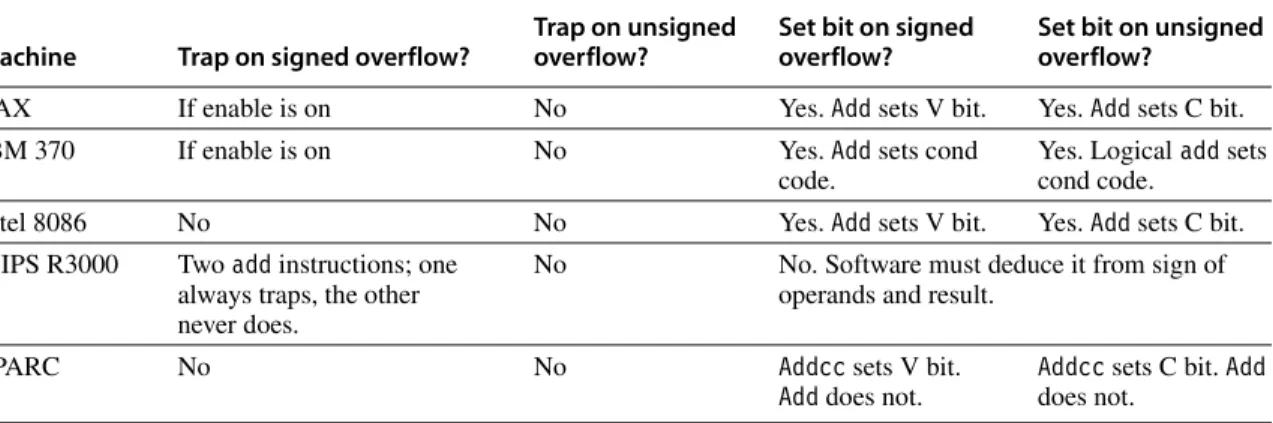
are signed or unsigned integers. Consider signed arithmetic first. There are three approaches: Set a bit on overflow, trap on overflow, or do nothing on overflow. In the last case, software has to check whether or not an overflow occurred. The most convenient solution for the programmer is to have an enable bit. If this bit is turned on, then overflow causes a trap. If it is turned off, then overflow sets a bit (or, alter- natively, have two different add instructions). The advantage of this approach is that both trapping and nontrapping operations require only one instruction. Further- more, as we will see in Section J.7, this is analogous to how the IEEE floating-point standard handles floating-point overflow. Figure J.5 shows how some common machines treat overflow.
What about unsigned addition? Notice that none of the architectures in Figure J.5 traps on unsigned overflow. The reason for this is that the primary use of unsigned arithmetic is in manipulating addresses. It is convenient to be able to subtract from an unsigned address by adding. For example, when n = 4, we can subtract 2 from the unsigned address 10 = 10102 by adding 14 = 11102. This gen- erates an overflow, but we would not want a trap to be generated.
A second issue concerns multiplication. Should the result of multiplying two n-bit numbers be a 2n-bit result, or should multiplication just return the low-order n bits, signaling overflow if the result doesn’t fit in n bits? An argument in favor of an n-bit result is that in virtually all high-level languages, multiplication is an operation in which arguments are integer variables and the result is an integer variable of the same type. Therefore, compilers won’t generate code that utilizes a double-precision result. An argument in favor of a 2n-bit result is that it can be used by an assembly language routine to substantially speed up multiplication of multiple-precision integers (by about a factor of 3).
A third issue concerns machines that want to execute one instruction every cycle. It is rarely practical to perform a multiplication or division in the same amount of time that an addition or register-register move takes. There are three possible approaches to this problem. The first is to have a single-cycle multiply- step instruction. This might do one step of the Booth algorithm. The second
Machine Trap on signed overflow?
Trap on unsigned overflow?
Set bit on signed overflow?
Set bit on unsigned overflow?
VAX If enable is on No Yes. Add sets V bit. Yes. Add sets C bit.
IBM 370 If enable is on No Yes. Add sets cond
code.
Yes. Logical add sets cond code.
Intel 8086 No No Yes. Add sets V bit. Yes. Add sets C bit.
MIPS R3000 Two add instructions; one always traps, the other never does.
No No. Software must deduce it from sign of operands and result.
SPARC No No Addcc sets V bit.
Add does not.
Addcc sets C bit. Add does not.
Figure J.5 Summary of how various machines handle integer overflow. Both the 8086 and SPARC have an instruction that traps if the V bit is set, so the cost of trapping on overflow is one extra instruction.
approach is to do integer multiplication in the floating-point unit and have it be part of the floating-point instruction set. (This is what DLX does.) The third approach is to have an autonomous unit in the CPU do the multiplication. In this case, the result either can be guaranteed to be delivered in a fixed number of cycles—and the compiler charged with waiting the proper amount of time—or there can be an interlock. The same comments apply to division as well. As examples, the original SPARC had a multiply-step instruction but no divide-step instruction, while the MIPS R3000 has an autonomous unit that does multiplica- tion and division (newer versions of the SPARC architecture added an integer multiply instruction). The designers of the HP Precision Architecture did an especially thorough job of analyzing the frequency of the operands for multi- plication and division, and they based their multiply and divide steps accordingly.
(See Magenheimer et al. [1988] for details.)
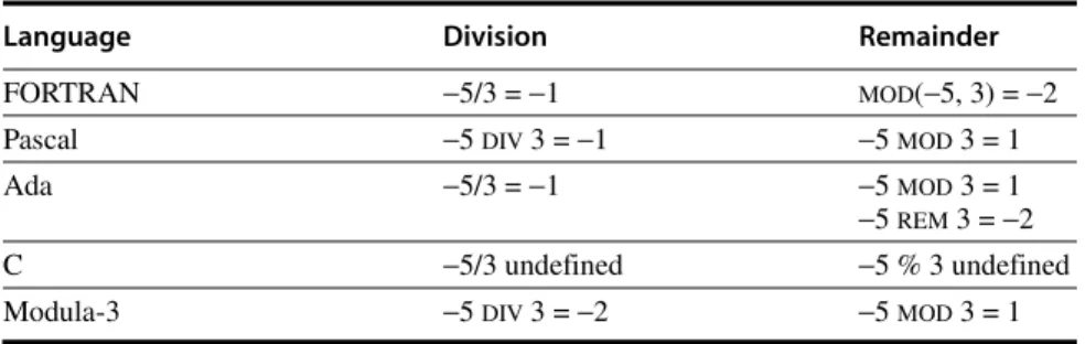
The final issue involves the computation of integer division and remainder for negative numbers. For example, what is −5 DIV 3 and −5 MOD 3? When comput- ing x DIV y and x MOD y, negative values of x occur frequently enough to be worth some careful consideration. (On the other hand, negative values of y are quite rare.) If there are built-in hardware instructions for these operations, they should correspond to what high-level languages specify. Unfortunately, there is no agreement among existing programming languages. See Figure J.6.
One definition for these expressions stands out as clearly superior, namely, x DIV y = ⎣x/y⎦, so that 5 DIV 3 = 1 and −5 DIV 3 = −2. And MOD should satisfy x = (x DIV y)×y + xMODy, so that x MOD y ≥ 0. Thus, 5 MOD 3 = 2, and −5 MOD 3 = 1. Some of the many advantages of this definition are as follows:
1. A calculation to compute an index into a hash table of size N can use MOD N and be guaranteed to produce a valid index in the range from 0 to N − 1.
2. In graphics, when converting from one coordinate system to another, there is no “glitch” near 0. For example, to convert from a value x expressed in a sys- tem that uses 100 dots per inch to a value y on a bitmapped display with 70 dots per inch, the formula y = (70 × x) DIV 100 maps one or two x coordinates into each y coordinate. But if DIV were defined as in Pascal to be x/y rounded to 0, then 0 would have three different points (−1, 0, 1) mapped into it.
3. x MOD 2k is the same as performing a bitwise AND with a mask of k bits, and x
DIV 2k is the same as doing a k-bit arithmetic right shift.
Language Division Remainder
FORTRAN −5/3 = −1 MOD(−5, 3) = −2
Pascal −5 DIV 3 = −1 −5 MOD 3 = 1
Ada −5/3 = −1 −5 MOD 3 = 1
−5 REM 3 = −2
C −5/3 undefined −5 % 3 undefined
Modula-3 −5 DIV 3 = −2 −5 MOD 3 = 1
Figure J.6 Examples of integer division and integer remainder in various program- ming languages.
J.3 Floating Point ■ J-13
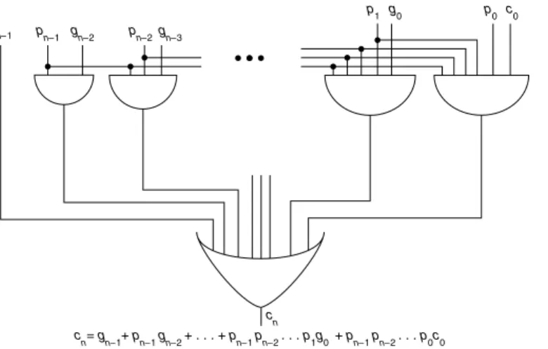
Finally, a potential pitfall worth mentioning concerns multiple-precision addition. Many instruction sets offer a variant of the add instruction that adds three operands: two n-bit numbers together with a third single-bit number. This third number is the carry from the previous addition. Since the multiple-precision number will typically be stored in an array, it is important to be able to increment the array pointer without destroying the carry bit.
Many applications require numbers that aren’t integers. There are a number of ways that nonintegers can be represented. One is to use fixed point; that is, use integer arithmetic and simply imagine the binary point somewhere other than just to the right of the least-significant digit. Adding two such numbers can be done with an integer add, whereas multiplication requires some extra shifting. Other representations that have been proposed involve storing the logarithm of a num- ber and doing multiplication by adding the logarithms, or using a pair of integers (a,b) to represent the fraction a/b. However, only one noninteger representation has gained widespread use, and that is floating point. In this system, a computer word is divided into two parts, an exponent and a significand. As an example, an exponent of −3 and a significand of 1.5 might represent the number 1.5 × 2–3
= 0.1875. The advantages of standardizing a particular representation are obvi- ous. Numerical analysts can build up high-quality software libraries, computer designers can develop techniques for implementing high-performance hardware, and hardware vendors can build standard accelerators. Given the predominance of the floating-point representation, it appears unlikely that any other representa- tion will come into widespread use.
The semantics of floating-point instructions are not as clear-cut as the seman- tics of the rest of the instruction set, and in the past the behavior of floating-point operations varied considerably from one computer family to the next. The varia- tions involved such things as the number of bits allocated to the exponent and sig- nificand, the range of exponents, how rounding was carried out, and the actions taken on exceptional conditions like underflow and overflow. Computer architec- ture books used to dispense advice on how to deal with all these details, but fortu- nately this is no longer necessary. That’s because the computer industry is rapidly converging on the format specified by IEEE standard 754-1985 (also an interna- tional standard, IEC 559). The advantages of using a standard variant of floating point are similar to those for using floating point over other noninteger represen- tations.
IEEE arithmetic differs from many previous arithmetics in the following major ways:
1. When rounding a “halfway” result to the nearest floating-point number, it picks the one that is even.
2. It includes the special values NaN, ∞, and −∞.
J.3 Floating Point
3. It uses denormal numbers to represent the result of computations whose value is less than 1.0 × 2Emin.
4. It rounds to nearest by default, but it also has three other rounding modes.
5. It has sophisticated facilities for handling exceptions.
To elaborate on (1), note that when operating on two floating-point numbers, the result is usually a number that cannot be exactly represented as another float- ing-point number. For example, in a floating-point system using base 10 and two significant digits, 6.1 × 0.5 = 3.05. This needs to be rounded to two digits. Should it be rounded to 3.0 or 3.1? In the IEEE standard, such halfway cases are rounded to the number whose low-order digit is even. That is, 3.05 rounds to 3.0, not 3.1.
The standard actually has four rounding modes. The default is round to nearest, which rounds ties to an even number as just explained. The other modes are round toward 0, round toward +∞, and round toward –∞.
We will elaborate on the other differences in following sections. For further reading, see IEEE [1985], Cody et al. [1984], and Goldberg [1991].
Special Values and Denormals
Probably the most notable feature of the standard is that by default a computation continues in the face of exceptional conditions, such as dividing by 0 or taking the square root of a negative number. For example, the result of taking the square root of a negative number is a NaN (Not a Number), a bit pattern that does not represent an ordinary number. As an example of how NaNs might be useful, con- sider the code for a zero finder that takes a function F as an argument and evalu- ates F at various points to determine a zero for it. If the zero finder accidentally probes outside the valid values for F, then F may well cause an exception. Writ- ing a zero finder that deals with this case is highly language and operating-system dependent, because it relies on how the operating system reacts to exceptions and how this reaction is mapped back into the programming language. In IEEE arith- metic it is easy to write a zero finder that handles this situation and runs on many different systems. After each evaluation of F, it simply checks to see whether F has returned a NaN; if so, it knows it has probed outside the domain of F.
In IEEE arithmetic, if the input to an operation is a NaN, the output is NaN (e.g., 3 + NaN = NaN). Because of this rule, writing floating-point subroutines that can accept NaN as an argument rarely requires any special case checks. For example, suppose that arccos is computed in terms of arctan, using the formula arccos x = 2 arctan( ). If arctan handles an argument of NaN properly, arccos will automatically do so, too. That’s because if x is a NaN, 1+x, 1−x, (1+x)/(1−x), and will also be NaNs. No checking for NaNs is required.
While the result of is a NaN, the result of 1/0 is not a NaN, but +∞, which is another special value. The standard defines arithmetic on infinities (there are both
1–x
( ) 1 x⁄( + ) 1–x
( ) 1 x⁄( + ) 1
–
J.3 Floating Point ■ J-15
+∞ and –∞) using rules such as 1/∞ = 0. The formula arccos x = 2 arc- tan( ) illustrates how infinity arithmetic can be used. Since arctan x asymptotically approaches π/2 as x approaches ∞, it is natural to define arctan(∞)
= π/2, in which case arccos(−1) will automatically be computed correctly as 2 arc- tan(∞) = π.
The final kind of special values in the standard are denormal numbers. In many floating-point systems, if Emin is the smallest exponent, a number less than 1.0 × 2Emincannot be represented, and a floating-point operation that results in a number less than this is simply flushed to 0. In the IEEE standard, on the other hand, numbers less than 1.0 × 2Emin are represented using significands less than 1.
This is called gradual underflow. Thus, as numbers decrease in magnitude below 2Emin, they gradually lose their significance and are only represented by 0 when all their significance has been shifted out. For example, in base 10 with four significant figures, let x = 1.234 × 10Emin. Then, x/10 will be rounded to 0.123 × 10Emin, having lost a digit of precision. Similarly x/100 rounds to 0.012 × 10Emin, and x/1000 to 0.001 × 10Emin, while x/10000 is finally small enough to be rounded to 0. Denormals make dealing with small numbers more predictable by maintain- ing familiar properties such as x = y ⇔ x − y = 0. For example, in a flush-to-zero system (again in base 10 with four significant digits), if x = 1.256 × 10Emin and y = 1.234 × 10Emin, then x − y = 0.022 × 10Emin, which flushes to zero. So even though x ≠ y, the computed value of x − y = 0. This never happens with gradual underflow.
In this example, x − y = 0.022 × 10Emin is a denormal number, and so the computa- tion of x − y is exact.
Representation of Floating-Point Numbers
Let us consider how to represent single-precision numbers in IEEE arithmetic.
Single-precision numbers are stored in 32 bits: 1 for the sign, 8 for the exponent, and 23 for the fraction. The exponent is a signed number represented using the bias method (see the subsection “Signed Numbers,” page J-7) with a bias of 127.
The term biased exponent refers to the unsigned number contained in bits 1 through 8, and unbiased exponent (or just exponent) means the actual power to which 2 is to be raised. The fraction represents a number less than 1, but the sig- nificand of the floating-point number is 1 plus the fraction part. In other words, if e is the biased exponent (value of the exponent field) and f is the value of the frac- tion field, the number being represented is 1. f × 2e–127.
Example What single-precision number does the following 32-bit word represent?
1 10000001 01000000000000000000000
Answer Considered as an unsigned number, the exponent field is 129, making the value of the exponent 129 − 127 = 2. The fraction part is .012 = .25, making the signifi- cand 1.25. Thus, this bit pattern represents the number −1.25×22 = −5.
1–x
( ) 1 x⁄( + )
The fractional part of a floating-point number (.25 in the example above) must not be confused with the significand, which is 1 plus the fractional part. The lead- ing 1 in the significand 1.f does not appear in the representation; that is, the leading bit is implicit. When performing arithmetic on IEEE format numbers, the fraction part is usually unpacked, which is to say the implicit 1 is made explicit.
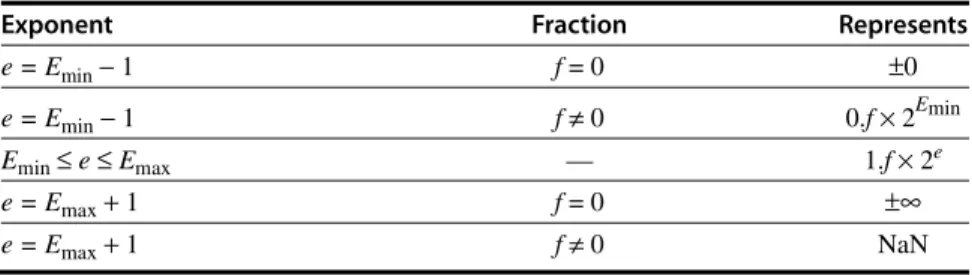
Figure J.7 summarizes the parameters for single (and other) precisions. It shows the exponents for single precision to range from –126 to 127; accordingly, the biased exponents range from 1 to 254. The biased exponents of 0 and 255 are used to represent special values. This is summarized in Figure J.8. When the biased exponent is 255, a zero fraction field represents infinity, and a nonzero fraction field represents a NaN. Thus, there is an entire family of NaNs. When the biased exponent and the fraction field are 0, then the number represented is 0.
Because of the implicit leading 1, ordinary numbers always have a significand greater than or equal to 1. Thus, a special convention such as this is required to represent 0. Denormalized numbers are implemented by having a word with a zero exponent field represent the number 0.f × 2Emin.
The primary reason why the IEEE standard, like most other floating-point formats, uses biased exponents is that it means nonnegative numbers are ordered in the same way as integers. That is, the magnitude of floating-point numbers can be compared using an integer comparator. Another (related) advantage is that 0 is represented by a word of all 0s. The downside of biased exponents is that adding them is slightly awkward, because it requires that the bias be subtracted from their sum.
Single Single extended Double Double extended
p (bits of precision) 24 ≥32 53 ≥64
Emax 127 ≥1023 1023 ≥16383
Emin −126 ≤−1022 −1022 ≤−16382
Exponent bias 127 1023
Figure J.7 Format parameters for the IEEE 754 floating-point standard. The first row gives the number of bits in the significand. The blanks are unspecified parameters.
Exponent Fraction Represents
e = Emin− 1 f = 0 ±0
e = Emin− 1 f ≠ 0 0.f × 2Emin
Emin≤ e ≤ Emax — 1.f × 2e
e = Emax+ 1 f = 0 ±∞
e = Emax+ 1 f ≠ 0 NaN
Figure J.8 Representation of special values. When the exponent of a number falls outside the range Emin≤ e ≤ Emax, then that number has a special interpretation as indi- cated in the table.
J.4 Floating-Point Multiplication ■ J-17
The simplest floating-point operation is multiplication, so we discuss it first. A binary floating-point number x is represented as a significand and an exponent, x = s × 2e. The formula
(s1 × 2e1) • (s2 × 2e2) = (s1 • s2) × 2e1+e2
shows that a floating-point multiply algorithm has several parts. The first part multiplies the significands using ordinary integer multiplication. Because floating- point numbers are stored in sign magnitude form, the multiplier need only deal with unsigned numbers (although we have seen that Booth recoding handles signed two’s complement numbers painlessly). The second part rounds the result.
If the significands are unsigned p-bit numbers (e.g., p = 24 for single precision), then the product can have as many as 2p bits and must be rounded to a p-bit num- ber. The third part computes the new exponent. Because exponents are stored with a bias, this involves subtracting the bias from the sum of the biased exponents.
Example How does the multiplication of the single-precision numbers 1 10000010 000. . . = –1 × 23
0 10000011 000. . . = 1 × 24 proceed in binary?
Answer When unpacked, the significands are both 1.0, their product is 1.0, and so the result is of the form:
1 ???????? 000. . .
To compute the exponent, use the formula:
biased exp (e1 + e2) = biased exp(e1) + biased exp(e2) − bias From Figure J.7, the bias is 127 = 011111112, so in two’s complement –127 is 100000012. Thus, the biased exponent of the product is
10000010
10000011
+ 10000001 10000110
Since this is 134 decimal, it represents an exponent of 134 − bias = 134 − 127 = 7, as expected.
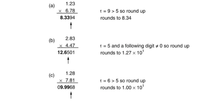
The interesting part of floating-point multiplication is rounding. Some of the different cases that can occur are illustrated in Figure J.9. Since the cases are sim- ilar in all bases, the figure uses human-friendly base 10, rather than base 2.
J.4 Floating-Point Multiplication