蟻群系統於單機單準則與多準則排程問題之應用(II)

行政院國家科學委員會專題研究計畫 成果報告

蟻群系統於單機單準則與多準則排程問題之應用(2/2)

計畫類別： 個別型計畫

計畫編號： NSC93-2213-E-011-014-

執行期間： 93 年 08 月 01 日至 94 年 07 月 31 日 執行單位： 國立臺灣科技大學工業管理系

計畫主持人： 廖慶榮

報告類型： 完整報告

處理方式： 本計畫涉及專利或其他智慧財產權，1 年後可公開查詢

中 華 民 國 94 年 10 月 26 日

行政院國家科學委員會專題研究計畫成果報告

蟻群系統於單準則與多準則排程問題之應用

Ant Colony Optimization for Scheduling Problems

with Single and Multiple Criteria

計畫編號：NSC-92-2213- E-011-058, NSC-93-2213-E-011-014 執行期限：92 年 8 月 1 日至 94 年 7 月 31 日

主持人：廖慶榮 教授 台灣科技大學工業管理系

計畫參與人員：曾兆堂 台灣科技大學企業管理系博士班

黃國凌 台灣科技大學工業管理系碩士班

阮曉健 台灣科技大學工業管理系碩士班 廖錚圻 台灣科技大學工業管理系碩士班

中文摘要

本 研 究 中 我 們 設 計 了 不 同 的 三 種 不 同 的 螞 蟻 族 群 最 佳 化 (Ant Colony Optimization；ACO) 演算法來求解單機單目標、單機多目標及零工型排程問題。本研 究主要區分為以下三部分：

Part I: ACO 求解考慮相依整備時間的單機環境下之排程問題

在實務界的生產系統中，相依整備時間 (sequence-dependent setups) 是排程不可或 缺的考慮因素，而其中總延遲時間一直被視為最重要的目標之一。但儘管相依整備時間 之延遲問題是如此的重要，過去的文獻卻鮮有相關的討論。因此在本論文中，我們利用 ACO 在單機環境下求解相依整備時間之延遲問題。我們提出的螞蟻演算法有一些不同 以往的特色，包括導入一個費洛蒙初始值的修正參數以及採用局部搜尋的時機等。我們 針對標竿問題來做測試，發現它的績效凌駕了許多其它的演算法；我們更進一步地將此 演算法應用在無權重的延遲問題上，實驗結果顯示，此演算法在面對其它擁有最佳表現 的演算法時，也能顯現出它的優勢。

Part II. ACO 求解單機多目標準則之排程問題

我們也嘗試將螞蟻演算法應用在求解最大完工時間以及總延遲時間的單機雙目標 問題上，並將它與一種派工法則 ATCS (Apparent Total Cost with Setups) 做比較，由實 驗結果得知，在此問題下，螞蟻演算法亦有相當優秀的表現。

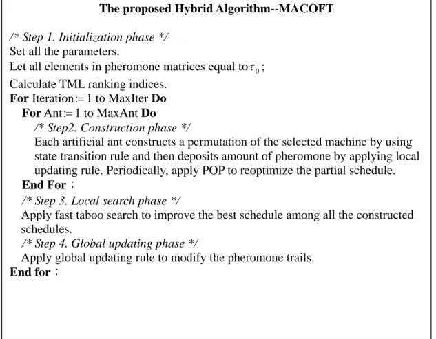
Part III. 混合以單機為基礎之 ACO 演算法與禁忌演算法來求解典型零工型排程問題 在此部分中，我們以瓶頸轉換法的分解概念作為基礎，將原本複雜的零工型排程問 題分解為多個單機問題來發展出一種以單機為基礎之 ACO 求解模式，並結合禁忌演算 法設計出一種混合型演算法。ACO 在許多組合問題上有許多相當不錯的發展，在零工 型排程問題的發展上仍屬初步，部分原因在於費落蒙收斂性過差。有鑑於此，我們設計 了一種新型的費落蒙陣列來提升 ACO 在此問題上的搜尋能力，輔以禁忌搜尋演算法來 提升求解品質，實驗解果顯示此混合演算法在標竿問題的求解中獲得相當良好的效果，

而與其他單一或混合演算法相比較，仍然具有相當良好的競爭力。

關鍵詞：排程、螞蟻演算法、相依整備時間、總延遲時間、雙目標、最大完工時間、零 工型排程、禁忌搜尋。

Abstract

In this research we develop three specific ant colony optimization (ACO) algorithms for single machine problem with single criterion and multiple criteria and for job shop scheduling problems. The research includes the following three parts:

Part I. Ant colony optimization for single machine tardiness scheduling with sequence- dependent setups.

In many real-world production systems, it requires an explicit consideration of sequence-dependent setup times when scheduling jobs. As for the scheduling criterion, the weighted tardiness is always regarded as one of the most important criteria in practical systems. While the importance of the weighted tardiness problem with sequence-dependent setup times has been recognized, the problem has received little attention in the scheduling literature. In this paper, we present an ant colony optimization (ACO) algorithm for such a problem in a single machine environment. The proposed ACO algorithm has several features, including introducing a new parameter for the initial pheromone trail and adjusting the timing of applying local search, among others. The proposed algorithm is experimented on the benchmark problem instances and shows its advantage over existing algorithms. As a further investigation, the algorithm is applied to the unweighted version of the problem.

Experimental results show that it is very competitive with the existing best-performing algorithms. Furthermore, we try to apply ACO algorithm to the single machine problem with bi-criteria of makespan and total weighted tardiness. The ACO algorithm is compared with the constructive-type heuristic of Apparent Tardiness Cost with Setups (ATCS) and its superiority is demonstrated.

Part II. Ant colony optimization for single machine scheduling problem with multiple objective scheduling criteria.

In this part we try to apply ACO algorithm to the single machine problem with bi-criteria of makespan and total weighted tardiness. The ACO algorithm is compared with the constructive-type heuristic of Apparent Tardiness Cost with Setups (ATCS) and its superiority is demonstrated.

Part III. Ant Colony Optimization combined with Taboo Search for the Job Shop Scheduling Problem

Following the conception of ACO in single machine problems, in this part we try to

decompose the job shop into several single machine problems and thus a single machine-based ACO combining with taboo search algorithm for the classical job shop scheduling problem is presented. ACO has been successfully applied to many combinatorial optimization problems, but obtained relatively uncompetitively computational results for this problem. To enhance the learning ability of ACO, we propose a specific pheromone trails definition inspired from the shifting bottleneck procedure and decompose the job shop scheduling into several single machine problems. Furthermore, we use a taboo local search to reinforce the schedules generated from the artificial ants. The proposed algorithm is experimented on 101 benchmark problem instances and shows its superiority over other novel algorithms. In particular, our proposed algorithm improves the upper bound on one open benchmark problem instance.

Keywords: Scheduling; Ant colony optimization; Weighted tardiness; Sequence- dependent setups; Taboo search; Job shop scheduling; Makespan; bicriterion.

Part I. Ant colony optimization for single machine tardiness scheduling with sequence-dependent setups

1. Introduction

The operations scheduling problems have been studied for over five decades. Most of these studies either ignored setup times or assumed them to be independent of job sequence [1]. However, an explicit consideration of sequence-dependent setup times (SDST) is usually required in many practical industrial situations, such as in the printing, plastics, aluminum, textile, and chemical industries [2, 3]. As Wortman [4] indicates, the inadequate treatment on SDST will hinder the competitive advantage.

On the other hand, a survey of US manufacturing practices indicates that meeting due dates is the single most important scheduling criterion [5]. Among the due-date criteria, the weighted tardiness is the most flexible one as it can be used to differentiate between customers.

While the importance of the weighted tardiness problem with SDST has been recognized, the problem has received little attention in the scheduling literature, mainly because of its complexity difficulty. This inspires us to develop a heuristic to obtain a near-optimal solution for this practical problem in the single machine environment. It is noted that the single machine problem does not necessarily involve only one machine; a complicated machine environment with a single bottleneck may be treated as a single machine problem.

We now give a formal description of the problem. We have

n

p ), due date (

d ), and weight (

w ). In addition, there is a setup time (

s )

j follows job i immediately in the processing sequence. Let Q be a

Q

Q Q

Q n , where Q k is the index of the

k

Q

The completion time of

Q k is

1

{

}

= ∑

+

Q k l Q l Q l Q l

C s p

Q k is

( ) =max{ ( )− ( ),

Q k Q k Q k

T C d

( ) ( )

=1

= ∑

Q k Q k Q k

WT w T

1/ s

/ ∑ w T

1/ ^s

/ ∑ ^T

Scheduling heuristics can be broadly classified into two categories: the constructive type

and the improvement type. In the literature the best constructive-type heuristic for the

1/ s

/ ∑ w T

1/ s

/ ∑ w T

1/ s

/ ∑ w T

1/ ^s

/ ∑ ^T

2. Literature review

2.1. Scheduling with sequence-dependent setup times

The importance of explicitly treating sequence-dependent setup times in production scheduling has been emphasized in the scheduling literature. In particularly, Wilbrecht and Prescott [7] states that this is particularly true where production equipment is being used close to its capacity levels. Wortman [4] states that the efficient management of production capacity requires the consideration of setup times.

2.2. 1/ ^s

/ ∑ ^T

^{and 1/ s}

^/ ∑ ^{w T}

Tardiness is a difficult criterion to work with even in the single machine environment.

There is no simple rule to minimize tardiness with sequence-independent set times, except for two special cases: (i) the Shortest Processing Time (SPT) scheduling minimizes total tardiness if all jobs are tardy, and (ii) the Earliest Due Date (EDD) scheduling minimizes total

tardiness if at most one job is tardy [8].Lawler et al. [9] show that the

1// ∑ w T

1/ s

/ ∑ w T

1/ ^s

/ ∑ ^T

s

C

NP-hard [13, p. 79] and

C

∑ T

Emmons [8] developed the dominance condition and solved two particular cases with constant setups. Lawler [9], among others, wrote on subject of the decomposition principle.

These contributions allowed the development of optimal solution procedures but they also inspired the construction of various heuristics.

Scheduling heuristics can be broadly classified into two categories: the constructive type and the improvement type [14, 15]. Construction techniques use dispatching rules to build a solution by fixing a job in a position at each step. These methods can select jobs for the sequence in a very simple or complex method. Simple methods may consist of sorting the jobs by the due date. More complex methods may be based on the specific problem structure.

These methods generally take fewer resources to find a solution but the solution tends to be erratic. Both of them are fast and highly efficient, but the quality of the solution in not very good. The dispatching rule might be a static one, i.e. time dependent like the earliest due date (EDD) rule, or a dynamic one, i.e. time dependent like the apparent tardiness cost (ATC) rule.

Vepsalainen and Morton [15] propose the ATC rule and test efficient dispatching rules for the weighted tardiness problem with specified due date and delay penalties.

In the literature the best constructive-type heuristic for the

1/ s

/ ∑ w T

In the second phase, the ranking indexes of all unscheduled jobs are computed and the job with the highest priority is sequenced. This procedure continues until all jobs are scheduled.

The third phase of the heuristic consists of a local search performed on a limited neighborhood, in which only the most promising moves are considered for evaluation.

However, like other constructive-type heuristics, ATCS can derive a feasible solution quickly but the solution quality is usually unsatisfactory, especially for large-sized problems. On the other hand, the improvement-type heuristic can produce better solutions but with much more computational efforts. For the

1/ s

/ ∑ w T

1/ s

/ ∑ w T

On the other hand, there exist several heuristics of the improvement type for the unweighted problem

1/ ^s

/ ∑ ^T

2.3. The ACO algorithm

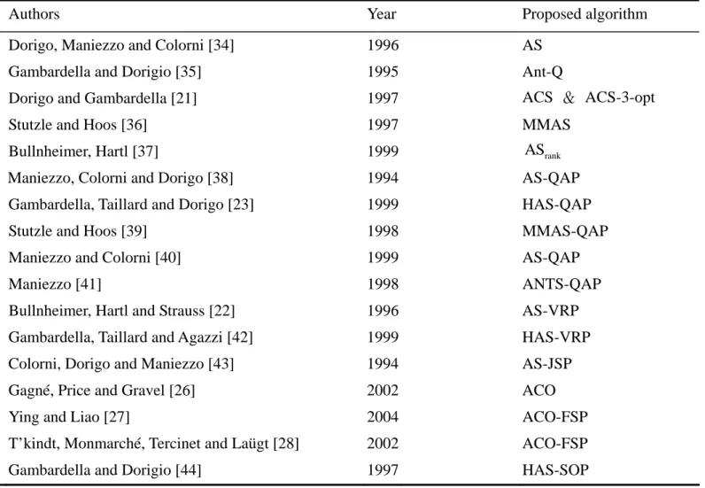
ACO has been successfully applied to a large number of combinatorial optimization problems, including traveling salesman problems [e.g., 21], vehicle routing problems [e.g., 22], and quadratic assignment problems [e.g., 23], which have shown the competitiveness with other metaheuristics. ACO has also been used successfully in solving scheduling problems on single machines [e.g., 24, 25, 26] and flow shops [e.g., 27, 28]. Table 1 lists the available implementations of ACO algorithms.

3. The background of ACO

ACO is inspired by the foraging behavior of real ants, which can be described as follows [33]. Real ants have the ability to find the shortest path from a food source to their nest without using visual cue. Instead, they communicate information about the food source through producing a chemical substance, called pheromone, laid on their paths. Since the shorter paths have a higher traffic density, these paths can accumulate higher amount of pheromone. Hence, the probability of ants following these shorter paths will be higher than the longer ones.

ACO is one of the metaheuristics for discrete optimization. One of the first applications of the ACO was to the solution of the traveling salesman problem (TSP) [21]. A matrix D of the distances

d i j between pairs ( i , j ) of cities is known and the objective is to find

Finally, the ant

k

k

We now describe details of the choice process: At time t the ant chooses the next city to visit considering a first factor called the trail intensity ( , )

τ

i j

τ

η

i j

d i j . This visibility acts as a greedy rule that favors the closest cities in the choice

p i j ,allows a

k

β

m

n

k

L

τ

i j

L

1 −

Table 1. Applications of ACO algorithm to combinatorial optimization problems

Problem type Authors Year Proposed algorithm

Traveling salesman Dorigo, Maniezzo and Colorni [34] 1996 AS

Gambardella and Dorigio [35] 1995 Ant-Q

Dorigo and Gambardella [21] 1997 ACS ＆ ACS-3-opt

Stutzle and Hoos [36] 1997 MMAS

Bullnheimer, Hartl [37] 1999 AS

Quadratic assignment Maniezzo, Colorni and Dorigo [38] 1994 AS-QAP Gambardella, Taillard and Dorigo [23] 1999 HAS-QAP

Stutzle and Hoos [39] 1998 MMAS-QAP

Maniezzo and Colorni [40] 1999 AS-QAP

Maniezzo [41] 1998 ANTS-QAP

Vehicle routing Bullnheimer, Hartl and Strauss [22] 1996 AS-VRP Gambardella, Taillard and Agazzi [42] 1999 HAS-VRP

Scheduling Colorni, Dorigo and Maniezzo [43] 1994 AS-JSP

Gagné, Price and Gravel [26] 2002 ACO

Ying and Liao [27] 2004 ACO-FSP

T’kindt, Monmarché, Tercinet and Laügt [28] 2002 ACO-FSP

Sequential ordering Gambardella and Dorigio [44] 1997 HAS-SOP

4. The proposed ACO algorithm

The ACO algorithm proposed in this paper is basically the ACS version [21], but it introduces the feature of minimum pheromone value from “max-min-ant system” (MMAS) [45]. Other elements of MMAS are not applied because there are no significant effects for the studied problem.

To make the algorithm more efficient and effective, we employ two distinctive features, along with three other elements used in some ACO algorithms. Before elaborating these features, we present our ACO algorithm as follows:

4.1. The step of the proposed ACO algorithm Step 0. Parameter description

Distance adjustment value ( β

Transition probability value (

q ):

q is a parameter between 0 and 1. It determines the

Decay parameter (

ρ

ρ

ρ ρ

Trail intensity ( ( , )

τ

i j

i j . Both the level of the trail and the probability are greater and will again

τ

i j

τ

Number of ants (

m

m

Step 1. Pheromone initialization

Let the initial pheromone trail

τ

K n WT

K is a parameter, n

WT

Step 2. Main loop

In the main loop, each of the

m

n

= 1000

Step 2.1. Constructing a job sequence by each ant

A set of artificial ants is initially created. Each ant starts with an empty sequence and then successively appends an unscheduled job to the partial sequence until a feasible solution is constructed (i.e., all jobs are scheduled). In choosing the next job j to be appended at the current position

i , the ant applies the following state transition rule:

[ ] [ ]

{ }

arg max ( , ) ( , ) if

otherwise

τ η

∈

⎧ ⋅ ≤

= ⎨⎪

⎪⎩

t 0

u U

i u i u q q

j

S

where ( , )

τ

i u

u

i at

t , U

q is a random number uniformly distributed in [0,1] ,

q is a parameter

q

q

q

S

S

[ ] [ ] [ ] [ ]

( , ) ( , )

( , )

( , ) ( , )

t

t u U

i j i j

p i j

i u i u

β β

τ η

τ η

∈

= ⋅

∑ ⋅

The parameter ( , )

η i j

β

η i j

I t v (i.e., set

( , )

i j I t v

η

1 2

max( , 0)

( , )

exp

exp

j

j

s

w d p t

I t v

p k p k s

− −

⎡ ⎤ ⎡ ⎤

= ⎢ − ⎥ ⎢ − ⎥

⎣ ⎦ ⎣ ⎦

where t denotes the current time,

w

p d are the weight, processing time, and due-date of job

j respectively, v

i − 1

k is the due date-related parameter, and

k is the setup time-related

Step 2.2. Local update of pheromone trail

To avoid premature convergence, a local trail update is performed. The update reduces the pheromone amount for adding a new job so as to discourage the following ants from choosing the same job to put at the same position. This is achieved by the following local updating rule:

( , ) (1 ) ( , ) 0

t

i j

i j

τ

ρ τ

ρ τ

ρ

ρ

Step 2.3. Local search

The local search in our algorithm is a combination of the interchange (IT) and the insert neighborhood (IS). The IT considers exchanges of jobs placed at the

i

Step 2.4. Global update of pheromone trail

The global updating rule is applied after each ant has completed a feasible solution (i.e., an iteration). Following the rule, the pheromone trail is added to the path of the incumbent global best solution, i.e., the best solution found so far. If job j is put at position i in the global best solution during iteration t , then

1( , )

t

i j

τ

α τ

i j

α τ

i j

where (0

α

α

t

i j WT

τ

Δ = , where

WT is the weight tardiness of the global best solution. In order to avoid

τ

i j

τ

4.2. The distinctive features

The above ACO algorithm has two distinctive features that make it competitive with other algorithms:

1. Introducing a new parameter for the initial pheromone trail.

2. Adjusting the timing of applying local search.

We first discuss the impact of introducing a new parameter for the initial pheromone trail

τ

0 1/(

n L

τ

L is the objective value of a solution obtained either randomly or through

τ

1/ s

/ ∑ w T

We thus introduce a new parameter K for

τ

τ

K n L

As for the second feature, we note that in conventional ACO algorithms the local search is executed for the global best solution once within each iteration even for those with no improvement.

In our algorithm, the local search is applied whenever a better solution is found during an iteration.

Hence, the local search may be applied more than once or completely unused in an iteration. The computational experiments given in Section 5 show that our approach can save consistently the computation time as many as four times without deteriorating the solution quality. The main reason is that the local search in our approach has a higher probability to generate a better solution because the search is performed on a less unexplored space.

In addition to the two features, there are also some useful elements which have been used in other ACO algorithms being employed in our proposed algorithm. These elements include

1. A lower bound for the pheromone trail. Stützle and Hoos [45] develop the so-called max-min ant system (MMAS) which introduces upper and lower bounds to the values of pheromone trail.

Based on our experiments, imposing a lower bound to the pheromone trail value improves the solution significantly, but there is no significant effect with an upper bound. Thus, only a lower bound is introduced in our algorithm.

2. A local search combining the interchange (IT) and the insert neighborhoods (IS). In our algorithm, the local search is a combination of IT and IS [25]. We use two of its variants, IT/IS and IS/IT, depending on which is implemented first. The choice of IT/IS or IS/IT is determined randomly in our algorithm.

3. The job-to-position definition of pheromone trail. In general, there are two manners to define the pheromone trail in scheduling, job-to-job [26] and job-to-position definitions. Based on our experimental analyses, the job-to-position definition is more efficient than job-to-job for the

1/ s

/ ∑ w T

5. Computational experiments

To verify the performance of the algorithm, two sets of computational experiments were conducted, one is for

1/ s

/ ∑ w T

1/ s

/ ∑ T

5.1. 1/ s

/ ∑ w T

In the first set of experiments (for

1/ s

/ ∑ w T

ζ

δ

R

ζ

For each combination, 10 problem instances each with 60 jobs were generated. The best known solutions to these instances were established by applying each of the following improvement-type heuristics: LDS (limited discrepancy search), HBSS (heuristic-biased stochastic sampling), VBSS (value-biased stochastic sampling), and VBSS-HC (hill-climbing using VBSS). According to the benchmark library, 27 such instances has been updated recently by a simulated annealing algorithm.

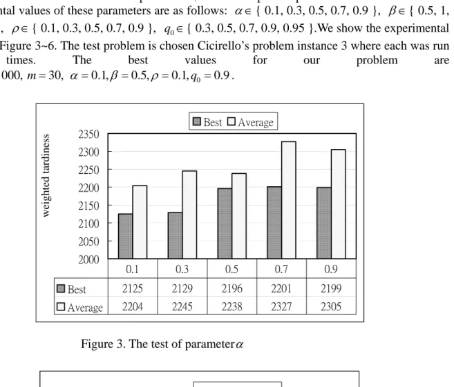
5.1.1. Parameters setting

To determine the best values of parameters, a series of pilot experiments was conducted. The experimental values of these parameters are as follows: α

∈

β

ρ

q

m

α

β

ρ

q

2000 2050 2100 2150 2200 2250 2300 2350

weighted tard iness

Best Average

Best 2125 2129 2196 2201 2199

Average 2204 2245 2238 2327 2305

0.1 0.3 0.5 0.7 0.9

Figure 3. The test of parameterα

1900 2000 2100 2200 2300 2400 2500

we ig h te d ta rd in e ss

Best Average

Best 2123 2135 2168 2157 2363 Average 2201 2225 2241 2285 2393

0.5 1 3 5 10

Figure 4. The test of parameter

β

2000 2050 2100 2150 2200 2250 2300 2350

weighted tardines s

Best Average

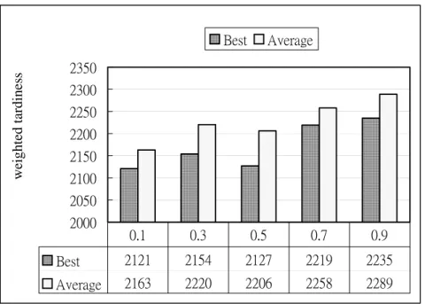
Best 2121 2154 2127 2219 2235 Average 2163 2220 2206 2258 2289

0.1 0.3 0.5 0.7 0.9

Figure 5. The test of parameter

ρ

1800 2000 2200 2400 2600 2800 3000

weighted tardiness

Best Average

Best 2799 2501 2294 2153 2165 Average 2958 2612 2477 2254 2302 0.3 0.5 0.7 0.9 0.95

Figure 6. The test of parameter

q

We now evaluate the impact of adding a new parameter K for the initial pheromone trail. To make a clear comparison, we temporarily remove the local search from the algorithm; all the other experiments in this paper were done with local search. Table 2 gives the computational results for 10 arbitrarily chosen Cicirello’s instances where each was run five times. Although there is no single best value of K for all the problem instances, good results can be obtained by setting

20

K =

K = 20

K = 20

Table 2.

The impact of introducing a parameter

K = 20

Average Best

Problem

K

K = 20

% to

=1

K K

K = 20

% to

=1

K

72 71694 69761 −2.7 69787 69657 −0.2

73 47322 45809 −3.2 46772 43242 −7.5

74 61158 49032 −19.8 59211 47809 −19.3 75 43518 39251 −9.8 43484 37291 −14.2 76 97201 72494 −25.4 88887 68361 −23.1 77 61302 52809 −13.9 58902 51940 −11.8 78 37598 34675 −7.8 37309 30274 −18.9 79 146437 134360 −8.2 142718 132398 −7.2 80 62990 45816 −27.3 58601 40266 −31.3

5.1.2. The test of local search

Another preliminary experiment was conducted to evaluate the timing of applying the local search. As noted earlier, in conventional ACO algorithms the local search is executed once for every iteration, but our algorithm applies the local search whenever a better solution is found. Table 3 gives the computational results for 10 arbitrarily chosen Cicirello’s instances where each was run five times. In the experiment, the only termination rule is set by letting Itemax

= 1000

Table 3.

The effect of timing for applying the local search

Average Best Time (sec.)

Problem Conv. New Conv. New Conv. New % 71 157328 + 160022 150521 + 157382 120.25 30.99 25.8 72 58011 57669 + 56364 56273 + 122.62 32.11 26.2 73 35989 + 36203 34932 + 35108 121.31 31.45 25.9 74 37267 37012 + 34508 + 34964 121.52 31.80 26.2 75 34305 32013 + 32990 29878 + 118.66 31.42 26.5 76 68225 67936 + 67084 65317 + 126.05 33.02 26.2 77 40113 + 40539 37247 + 37896 121.89 33.14 27.2 78 28987 25998 + 27308 25213 + 123.52 31.84 25.8 79 126553 125293 + 123905 123408 + 125.92 32.59 25.9 80 28488 + 29033 27401 + 27796 130.30 34.30 26.3

* Conv.: the conventional approach; New: the new approach used in our algorithm

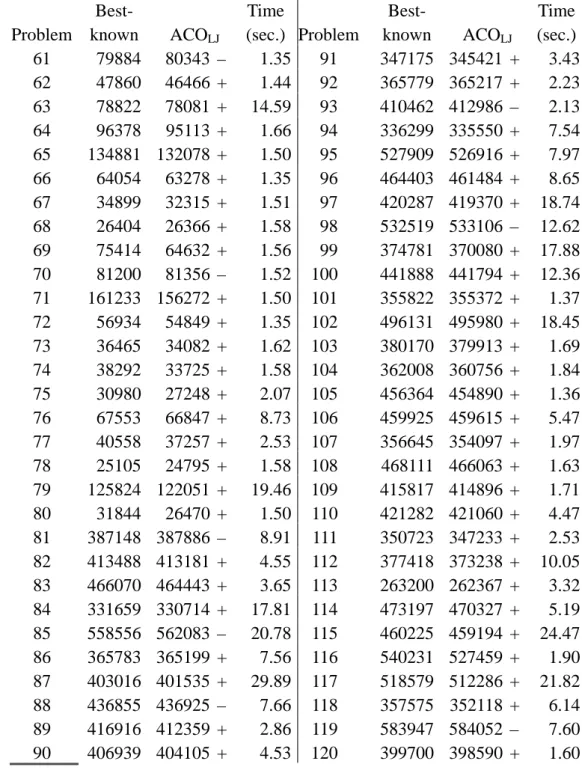
5.1.3. Results and discussions

We now present the formal experimental results for

1/ s

/ ∑ w T

selected. For the 104 instances with non-zero weighted tardiness, ACO_LJ has produced a better solution in 90 such instances (86%). For those with zero weighted tardiness, ACOLJ also has obtained the optimal solution. The average computation time for each run is only 4.99 seconds with 16 instances taking more than 10 seconds. The comparison of computation times cannot be made because they are not provided in the benchmark library.

Table 4.

Comparison of the solutions from the proposed ACOLJ with the best-known solutions

Problem

Best-

known ACOLJ

Time

(sec.) Problem

Best-

known ACOLJ

Time (sec.)

1 978 894 + 1.35 31 0 0 0†

2 6489 6307 + 1.33 32 0 0 0†

3 2348 2003 + 1.34 33 0 0 0†

4 8311 8003 + 2.05 34 0 0 0†

5 5606 5215 + 1.56 35 0 0 0†

6 8244 5788 + 4.48 36 0 0 0†

7 4347 4150 + 1.35 37 2407 2078 + 3.70

8 327 159 + 8.04 38 0 0 0†

9 7598 7490 + 2.69 39 0 0 0†

10 2451 2345 + 1.74 40 0 0 0†

11 5263 5093 + 6.46 41 73176 73578 – 7.57 12 0 0 12.08 42 61859 60914 + 1.49 13 6147 5962 + 8.43 43 149990 149670 + 1.74 14 3941 4035 – 7.09 44 38726 37390 + 1.33 15 2915 2823 + 27.45 45 62760 62535 + 2.21 16 6711 6153 + 2.64 46 37992 38779 – 1.67 17 462 443 + 6.14 47 77189 76011 + 7.53 18 2514 2059 + 4.12 48 68920 68852 + 2.31 19 279 265 + 5.29 49 84143 81530 + 1.35 20 4193 4204 – 1.35 50 36235 35507 + 1.58

21 0 0 0† 51 58574 55794 + 2.32

22 0 0 0† 52 105367 105203 + 8.35

23 0 0 0† 53 95452 96218 – 6.44

24 1791 1551 + 0† 54 123558 124132 – 3.63

25 0 0 0† 55 76368 74469 + 2.71

26 0 0 0† 56 88420 87474 + 1.80

27 229 137 + 1.762 57 70414 67447 + 5.13 28 72 19 + 1.803 58 55522 52752 + 1.47

29 0 0 0† 59 59060 56902 + 9.18

30 575 372 + 8.49 60 73328 72600 + 12.54

(Continued on next page)

Table 4 (Continued)

Problem

Best-

known ACOLJ

Time

(sec.) Problem

Best-

known ACOLJ

Time (sec.) 61 79884 80343 – 1.35 91 347175 345421 + 3.43 62 47860 46466 + 1.44 92 365779 365217 + 2.23 63 78822 78081 + 14.59 93 410462 412986 – 2.13 64 96378 95113 + 1.66 94 336299 335550 + 7.54 65 134881 132078 + 1.50 95 527909 526916 + 7.97 66 64054 63278 + 1.35 96 464403 461484 + 8.65 67 34899 32315 + 1.51 97 420287 419370 + 18.74 68 26404 26366 + 1.58 98 532519 533106 – 12.62 69 75414 64632 + 1.56 99 374781 370080 + 17.88 70 81200 81356 – 1.52 100 441888 441794 + 12.36 71 161233 156272 + 1.50 101 355822 355372 + 1.37 72 56934 54849 + 1.35 102 496131 495980 + 18.45 73 36465 34082 + 1.62 103 380170 379913 + 1.69 74 38292 33725 + 1.58 104 362008 360756 + 1.84 75 30980 27248 + 2.07 105 456364 454890 + 1.36 76 67553 66847 + 8.73 106 459925 459615 + 5.47 77 40558 37257 + 2.53 107 356645 354097 + 1.97 78 25105 24795 + 1.58 108 468111 466063 + 1.63 79 125824 122051 + 19.46 109 415817 414896 + 1.71 80 31844 26470 + 1.50 110 421282 421060 + 4.47 81 387148 387886 – 8.91 111 350723 347233 + 2.53 82 413488 413181 + 4.55 112 377418 373238 + 10.05 83 466070 464443 + 3.65 113 263200 262367 + 3.32 84 331659 330714 + 17.81 114 473197 470327 + 5.19 85 558556 562083 – 20.78 115 460225 459194 + 24.47 86 365783 365199 + 7.56 116 540231 527459 + 1.90 87 403016 401535 + 29.89 117 518579 512286 + 21.82 88 436855 436925 – 7.66 118 357575 352118 + 6.14 89 416916 412359 + 2.86 119 583947 584052 – 7.60 90 406939 404105 + 4.53 120 399700 398590 + 1.60 + The proposed algorithm is better.

– The proposed algorithm is worse.

†Computation time less than 0.1 second for each of 10 runs.

5.2. 1/ s

/ ∑ T

These favorable computational results encourage us to apply our ACO_LJ algorithm to the unweighted problem

1/ s

/ ∑ T

1/ s

/ ∑ T

1/ s

/ ∑ T

5.2.1. The small and medium-sized problems

To test the small and medium-sized problems (with 15-45 jobs), we use the 32 test problem instances provided by Rubin and Ragatz [6] which can be obtained at http://mgt.bus.msu.edu/datafiles.htm. Table 5 shows the comparison among RSPI, ACOGPG, and ACO_LJ (the result of Tabu-VNS is not available for the small-sized problems), where ACO_GPG gives the best solution from 20 runs and ACOLJ gives the best solution from 10 runs. All the three algorithms find the optimal solutions for those 16 instances whose optimal solutions are known. For the remaining 16 instances, the three algorithms (RSPI, ACO_GPG, and ACO_LJ) find the best solutions for 2 (13%), 3 (19%), and 15 (94%) such instances, respectively; three instances end in a tie.

To evaluate the degree of difference in performance, we calculate the percentage difference for each of those instances whose solutions are different by ACOGPG and ACOLJ. The results are given in the last columns of table 5. A positive value of percentage difference indicates that the ACO_GPG is better while a negative value indicates that ACOLJ is better. ACOLJ shows an average percentage improvement of 1.71% for small-sized problems .

5.2.2. The large-sized problems

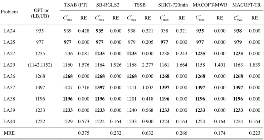
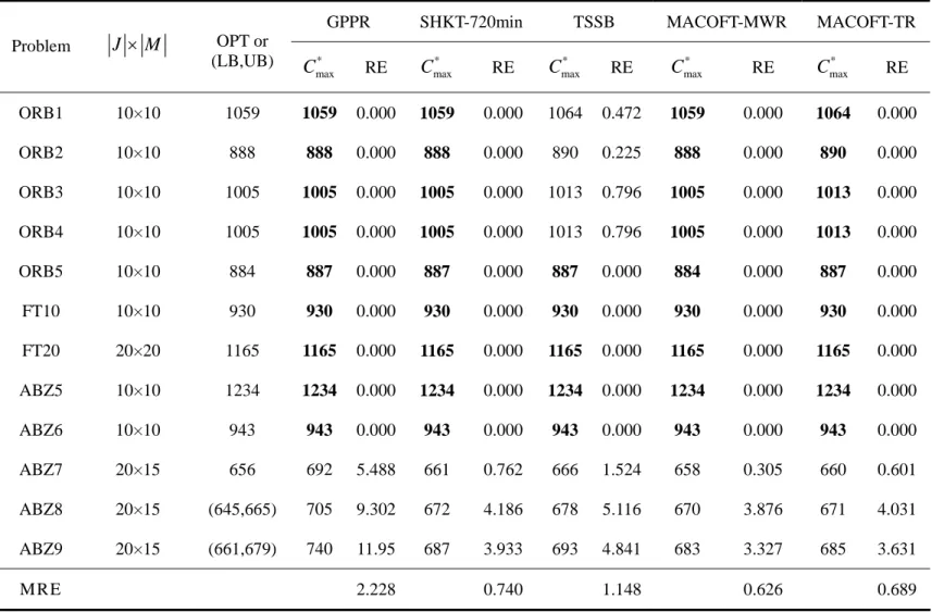
To test the large-sized problems (with 55-85 jobs), we use the test problem instances provided by Gagné et al. [26] and make the comparison among ACO_GPG, Tabu-VNS, and ACO_LJ. Both ACOGPG and ACOLJ give their best solutions from 20 runs. To make our ACOLJ algorithm more efficient and effective, some of its parameters were fine tuned:

β

q

K

We simply note that the average computation time of each run for our ACO_LJ is 24.17 seconds for all the 32 instances.