可靠度導向之隨機流量網路最佳化資源配置研究

行政院國家科學委員會專題研究計畫 成果報告

可靠度導向之隨機流量網路最佳化資源配置研究(第 3 年) 研究成果報告(完整版)

計 畫 類 別 ： 個別型

計 畫 編 號 ： NSC 96-2628-E-011-116-MY3

執 行 期 間 ： 98 年 08 月 01 日至 99 年 07 月 31 日 執 行 單 位 ： 國立臺灣科技大學工業管理系

計 畫 主 持 人 ： 林義貴

計畫參與人員： 博士班研究生-兼任助理人員：葉承達

報 告 附 件 ： 出席國際會議研究心得報告及發表論文

處 理 方 式 ： 本計畫涉及專利或其他智慧財產權，2 年後可公開查詢

中 華 民 國 99 年 10 月 19 日

行政院國家科學委員會補助專題研究計畫 ■ 成 果 報 告

□期中進度報告 可靠度導向之隨機流量網路最佳化資源配置研究

計畫類別：個別型計畫 □整合型計畫 計畫編號：NSC 96-2628-E-011-116-MY3 執行期間： 96 年 8 月 1 日至 99 年 7 月 31 日

執行機構及系所：

計畫主持人：林義貴 教授 共同主持人：

計畫參與人員：葉承達 博士班研究生 許璧麗 碩士班研究生

成果報告類型(依經費核定清單規定繳交)：□精簡報告 完整報告

本計畫除繳交成果報告外，另須繳交以下出國心得報告：

□赴國外出差或研習心得報告

□赴大陸地區出差或研習心得報告

■出席國際學術會議心得報告

□國際合作研究計畫國外研究報告

處理方式：除列管計畫及下列情形者外，得立即公開查詢

■涉及專利或其他智慧財產權，□一年■二年後可公開查詢

中 華 民 國 99 年 8 月 27 日

目錄

目錄...I 中文摘要... II Abstract ... II

一、前言與目的...1

二、研究方法...1

1. Assumptions and notations ...1

2. Multi-commodity stochastic-flow network... 2

3. Problem formulation ... 5

4. GA based approach development... 6

四、結果與討論...7

1. Example: a practical logistic network ... 7

2. Conclusion and discussion ... 11

參考文獻...12

國科會補助專題研究計畫成果報告自評表...144

國科會補助計畫衍生研發成果推廣資料表...15

國科會補助專題研究計畫項下出席國際學術會議心得報告...17

出席國際學術會議發表之論文...21

中文摘要

本三年期計畫處理的網路，其每個傳輸邊與節點上具有多個資源可供配置，每個資源有多 種狀態，每個狀態代表不同的容量（capacity），當網路上的邊與節點配置這些具有多種狀態的 資源時，則網路為一隨機型流量網路。本計畫考量因素則包含：資源的「容量」與「傳輸時間」、

「傳輸時間」、「多商品」及「節點失效」，其中容量與傳輸時間為隨機變數。每項因素都是 重要且需要複雜的研究步驟，故將此一計畫分為三年執行。在終點處已提出需求量之要求下，

系統可靠度為系統可以從起點至終點成功傳輸商品量之機率，如何配置此些資源以使系統可靠 度得到最大值便為本計畫之目標。本三年期計畫利用基因演算法找出最佳的資源配置，而系統 可靠度之計算則是藉由最小路徑之網路特性以及遞迴不交合法 (Recursive Sum of Disjoint Products，RSDP)所求得，而所發展之模式，則近一步探討如何應用在物流網路中。

關鍵詞：資源配置、最佳系統可靠度、傳輸成本、多商品、基因演算法

Abstract

The purpose of the 3-year project is to study the resource allocation in order to maximize the system reliability. Each resource has several states which represent the possible capacities. The network associated with any resource allocation is a stochastic-flow network. This plan considers the factors including transmission cost, transmission time, multi-commodity and node failure, in which the capacity and is stochastic. Since the steps which each factor involves are very complicated, this plan is executed in three years. The system reliability is the probability that the network associated with the resource allocation can satisfy the given units of multi-commodity demand subject to a budget. How to allocate the existing resources to the network such that the system reliability is maximized is the objective of the plan. The 3-year project utilizes the genetic algorithm to search for the optimal resource allocation with maximal system reliability. The system reliability is evaluated by the minimal paths and the Recursive Sum of Disjoint Products.

Key Words: Resources allocation, maximal system reliability, transmission cost, multi-commodity, genetic algorithm.

一、前言與目的

傳統之網路分析遇到流量（flow）、傳輸成本等因素時，大多為分開處理，並且大多將此 些因素設為確定性模式（deterministic）。然而，由於維修、故障、被預約等因素，站在客戶的 觀點而言，許多實際的流量網路如電腦系統、電信系統、物流系統、交通運輸系統等，其傳輸 邊的容量應視為隨機性（stochastic）方較合理，因為客戶可以使用的容量受限於前述因素不見 得都是一成不變。此種流量網路稱之為隨機型流量網路（stochastic-flow network）[1,9-24]。舉 例而言，電腦系統為其中一種代表性網路，以每部電腦（或交換機）代表網路之節點，傳輸線 視為網路之傳輸邊。而傳輸線由多條實體網路線（如 T1 電纜、E1 電纜、光纖等）組成，每條 實體網路線只有正常與失效兩種情況；所以每條傳輸線會有數種狀態（state），狀態 k 表示有 k 條實體網路線正常。因此每個傳輸邊的容量會有數種可能值，自然導致系統的最大流量會有多 種可能，因而系統本身也是多種狀態。

近年來，如何將現有之資源配置於系統上，以達成最佳化之系統可靠度已成為另一重要之 課題。已有多位學者[2-8]針對隨機型網路進行最佳化可靠度之相關議題研究。此外，諸如文獻 [7]探討 k-out-of-r-from-n 的系統，系統中 r 個元件的績效總和小於一需求值則定義為系統失效，

利用基因演算法（Genetic algorithm）找出最佳的配置；文獻[8]則考量訊號傳輸有時間因素，系 統可靠度定義為時間限制內成功傳輸訊號的機率。然而在上述的最佳化可靠度議題中，僅考慮 起點與終點能連通（connect）的機率，並未將流量因素列入考量。就隨機型流量網路而言，Levitin [4]定義系統可靠度為商品能夠從起點至終點被成功傳送的機率。由於每個資源本身的狀態機率 分佈不盡相同，不同之配置會造成系統可靠度之差異，因而找出最好的配置規則以達成最大系 統可靠度為極有意義之議題。

本三年的研究以最小路徑特性考慮配置資源的「容量」與「成本」，以及「多商品」、「節 點失效」等因素，其中每一資源之容量為隨機變數。對於於每一傳輸邊及節點分別配置一資源，

並求算該組資源配置下，系統能夠傳送特定需求量及滿足預算限制之系統可靠度。在求算任一 組資源配置時，可利用最小路徑之網路特性與遞迴不交合法則可計算該組資源配置下之系統可 靠度，而利用基因演算法的程序逐步找出最佳之資源配置解，以得出最高之系統可靠度。

二、研究方法

1. Assumptions and notations

Let (N, R) be a network where N denotes the set of nodes, R = {ri|1 ≤ i ≤ n} denotes the set of n routes connecting two nodes. The MPs of (N, R) are designated as p1, p2, …, pm and the demand of u commodities at sink t is designated as D = (d1, d2, …, du) where dkis the demand of commodity k. Let W_i = {w_ie|1 ≤ e ≤z_i} be the set of z_i resources on route r_i for i = 1, 2, …, n, in which w_ie is the eth resource on route ri. Each resource wie has multiple states,1,2,…,Mie, with corresponding available capacities, 0 = hie(1) < hie(2) < … < hie(Mie) for e = 1, 2, …, zi, in which hie(l) is the lth capacity of wie

for l = 1,2,…,Mie. The cost ciemeans the cost per unit of capacity provided by resource wieon route ri. A resource allocation is designated as B = (b1, b2,…,bn) where bi= e if resource wieis selected to ship

stochastic-flow network. Several necessary assumptions for the stochastic-flow network for are listed as follows:

I. Flow in (N, R) must satisfy the flow-conservation principle. That is, no flow will be decreased or be increased during the delivery.

II. The capacities of different resources are statistically independent.

III. Different commodities should not be loaded in the same capacity.

Furthermore, xis the ceiling function which means the smallest integer such that xx. xis the floor function which means the greatest integer such thatxx.

2. Multi-commodity stochastic-flow network

The maximal capacity on route ri denoted by hib_i(Mib_i) is equal to hⁱε(Miε) if bi = εwhere ε{1, 2, …, zi} for i = 1, 2, …, n. Let MB = (h1b₁(M1b₁), h2b₂(M2b₂),…,hnb_n(Mnb_n)) be the maximal capacity vector associated with resource allocation B. Let X = (x₁, x₂, …, x_n) be a current capacity vector of (N, R) where xiis the current capacity on route ri. Any capacity vector X which is feasible associated with B meets the following constraint:

XM_B. (1)

Constraint (1) means the current capacity xi should not exceed the maximal capacity on route rifor i = 1, 2, …, n. For convenience, let U_B= {X|XM_B} be the set of all feasible X associated with B.

Let F = (f11, f12, …, f1m, f21, f22, …, f2m, …, fu1, fu2, …, fum) be a flow vector where fkj is the flow of commodity k through pj. The consumed capacity by per commodity k denoted by qkfor k = 1, 2, …, u is a real number. Under capacity vector MB, the amount of commodity k through route ri is bounded by

hib_i(Mib_i)/qk. Thus, any F satisfying the following constraints is said to be feasible under capacity vector MB.

1 :

( )

i i

i j

u

k kj ib ib

k

j r p

q f h M

 

  

  

  

 

 

for i = 1, 2,…,n, and (2)

where

:_{i j} kj j r p

f



 is the flow of commodity k traveling through route ri,

:_{i j}

k kj

j r p

q f



 

 

 





is the consumed capacity on ri by commodity k, and ₁

:_{i j} u

k kj

k

j r p

q f

 

  

  

  

 

 

is the total consumed capacity on ri by all commodities. Constraint (2) means the consumed capacity on route r_i should not exceed the maximal capacity of route rifor i = 1,2,…,n.

For convenience, let FM_Bdenote the set of all feasible F under MB. Similarly, let FX denote the set

of all F satisfying the following constraint:

1

:_{i j} u

k kj i

k

j r p

q f x

 

  

  

  

 

 

for i = 1, 2,…,n. (3)

Any capacity vector X is said to meet the demand D and the budget C if and only if there exists a flow vector FFXsatisfying the following constraints:

m

kj k

j

f d



for k = 1, 2, …, u, and (4)

1 1

:

i

i j

n u

ib k kj

i k

j r p

c q f

 



  

  

  

 

  

^{C. (5)}

where _{1 1}

:

i

i j

n u

ib k kj

i k

j r p

c q f

 



  

  

  

 

  

is the cost of the total flow traveling through route ri. For convenience, let XB = {X|X U_B satisfies the demand D and the budget C}. The system reliability associated with resource allocation B denoted by RD,C(B) is the probability that the demand D can be successfully shipped from s to t through the logistics network associated with B subject to budget C.

That is, RD,C(B) = Pr( )

X_B X



X .

A (B,D,C)-MP is defined to improve the computational efficiency of system reliability measurement.

Definition 1. A (B,D,C)-MP is a capacity vector XX_Bsuch that YX_Bfor any Y < X (where Y ≤X:

(y1, y2,…,yn) ≤(x1, x2,…,xn) if and only if yi≤ xifor each i; Y < X if and only if Y ≤X and y_i< xifor at least one i.)

Equivalently, any (B,D,C)-MP X is the maximal capacity vector in XB. Suppose there are totally v (B,D,C)-MPs: X1, X2,…,Xv. Then, XB=

1

{ { | , }}

v

i B

i

X X X X



 U



^{. Thus,}

RD,C(B) = Pr( )

X_B X



X

= Pr{

1 v

i{X|X Xi, XUB}}. (6)

Such a probability can be calculated by the RSDP. The RSDP is presented as the following pseudo codes.

The RSDP

function RSDP(X1, X2,…,Xv) //Input v capacity vectors for (i = 1; iv; i++)

if i == 1

Reliability = Pr(X ≥ Xi);

else

MRA = Pr(X ≥Xi);

if i == 2

MRB = Pr(X ≥max(X1, Xi)); //max(x1k, xik) for k = 1, 2, ..., n else

for (j = 1; ji –1; j++)

Xj= max(Xj, Xi); //max(xjk, xik) for k = 1, 2, ..., n end

v = v –1

MRB = RSDP(X1, X2,…,Xv); //Execute recursive procedure end

end

Reliability = Reliability + MRA –MRB; //Return system reliability end

Any flow vector F  F_M

B is said to meet the exact demand D and budget C if it satisfies constraints (5) and (7):

m

kj k

j

f d



for k = 1, 2, …, u. (7)

Let ΦB = {F|F F_M

B meets constraints (5) and (7)} be the set of F satisfying exact D subject to C under MB. A necessary condition for any (B,D,C)-MP is illustrated in the following theorem.

Theorem 1. If XU_Bis a (B,D,C)-MP, then there exists a feasible FΦ_Bsuch that xi= hib_i(l) where l {1,2,…,M_ib

i} and hib_i(l ﹣1) < ₁

:_{i j} u

k kj

k

j r p

q f

 

  

  

  

 

 

^hibi(l) for i = 1,

2,…,n. (8)

Proof. Let X be a (B,D,C)-MP and an FΦ_B∩F_X. Suppose to the contrary that there exists a route rπ

with xπ> hπb_π(l) ≥

1

: _j u

k kj

k

j r p

q f



 

  

  

  

 

 

^{and xi = hib}i(l) ≥

1

:_{i j} u

k kj

k

j r p

q f

 

  

  

  

 

 

^i ≠π.Set Y = (y₁, y2, …, yn) with yπ= hπb_π(l) and yi = xi  i ≠π. Thus, Y < X and F is feasible under Y due to

1

:_{i j} u

k kj

k

j r p

q f

 

  

  

  

 

 

^{yifor i = 1,2,…,}n. It infers YΦ_Band contradicts that X is a (B,D,C)-MP.



Based on Theorem 1, we transform each flow vector FΦ_Binto a capacity vector X through Eq.

(9). Such a capacity vector X is treated as a (B,D,C)-MP candidate. Let ΓB= {X|X is transformed from FΦ_Bvia Eq. (8)} be the set of such (B,D,C)-MP candidates, and Γ_B,minbe the set of minimal vectors in ΓB. The following theorem shows that ΓB,minis equivalent to the set of (B,D,C)-MPs.

Theorem 2. ΓB,minis equivalent to the set of (B,D,C)-MPs.

Proof. Suppose X  ΓB,min that means X  XB but it is not a (B,D,C)-MP. Hence, there exists a (B,D,C)-MP Y such that Y < X. That is, YΓ_Bwhich contradicts XΓ_B,min. Conversely, suppose X is a (B,D,C)-MP but XΓ_B,min. It is known X Γ_Bbased on Theorem 1. There exists a YΓ_Bsuch that Y

< X. It is given that Y X_B which contradicts that X is a (B,D,C)-MP. We therefore conclude ΓB,min is the set of (B,D,C)-MPs. 

Based on Theorem 2, whether (B,D,C)-MP candidates are (B,D,C)-MPs is identified by the following algorithm.

The (B,D,C)-MPs generation algorithm. //Check which capacity vectors in ΓBare (B,D,C)-MPs.

1) I =  (I is the stack which stores the indexes of the capacity vectors in Γ_B which are not a (B,D,C)-MP. Initially, I is empty.)

2) For i = 1 to |ΓB| & iI. //|Γ_B| means the number of capacity vectors in ΓB. 3) For j = i + 1 to |ΓB|, & jI.

4) If Xj< Xi, then Xiis not a (B,D,C)-MP, I = I ∪ {i}, and go to step 7.

Else X_jis not a (B,D,C)-MP, I = I ∪ {j}.

5) Next j.

6) Xiis a (B,D,C)-MP.

7) Next i.

3. Problem formulation

The mathematical program of the discussed problem is thus given by Max RD,C(B) = Pr{

1 v

i{X|X Xi, XUB}} (9)

Subject to

bi= e e {1,2,…,zi} for i = 1,2,…,n. (10)

Constraint (10) says route ri must be assigned exact one resource from set Wi for i = 1,2,…,n. All feasible resource allocations are found subject to constraint (10). Note that RD,C(B) = 0 if XB

=

1

{ { | , }}

v

i B

i

X X X X



 U



⁼ . The optimal resource allocation with maximal system reliability subject to budget C is obtained by maximizing objective function (9).

4. GA based approach development

The following steps describe the procedure of implementing the GA to solve the discussed problem.

1) Initially, set θ(population size), α(crossover rate), β(mutation rate), and λ(number of generations) and let count = 1. //count is utilized to count how many generations the GA runs.

2) Generate initial population with θchromosomes by using the integer representation.

3) Compute RD,C(G) for each chromosome G by the following algorithm: //Chromosome G is equivalent to resource allocation B.

3.1) Find all F satisfying the following constraints:

1 :

( )

i i

i j

u

k kj ig ig

k

j r p

q f h M

 

  

  

  

 

 

for i = 1, 2,…,n, and (11)

1 1

:

i

i j

n u

ig k kj

i k

j r p

c q f

 



  

  

  

 

  

^{C, (12)}

m

kj k

j

f d



for k = 1, 2, …, u. (13)

If there is no F satisfying constraints (11) — (13), a small value is assigned to be the chromosome’s system reliability and then to evaluate the next chromosome.

3.2) Transform each F into (G,D,C)-MP candidate X via the following equation:

xi= hig_i(l) where l {1,2,…,M_ig

i} and hig_i(l ﹣1) < ₁

:_{i j} u

k kj

k

j r p

q f

 

  

  

  

 

 

^higi(l) for i = 1,

2,…,n. (14)

3.3) Utilize the (G,D,C)-MPs generation algorithm to identify which (G,D,C)-MP candidates are (G,D,C)-MPs. //(G,D,C)-MP is (B,D,C)-MP since G is equivalent to B.

3.4) Suppose there are v (G,D,C)-MPs. Evaluate RD,C(G) = Pr{

1 v

i{X|X Xi, X UG}} by the RSDP.

4) If count > λ, return the optimal solution of the λth generation and stop the GA-MPRSDP.

Else if countλ,count = count + 1 and go to step 5.

5) Execute the evolution process

5.1) Employ the roulette wheel selection to select two chromosomes.

5.2) Implement the crossover uniform based on α. 5.3) Implement the uniform mutation based on β.

6) Use the two new chromosomes from step 5 to replace the two worst ones in the original population.

7) Calculate RD,C(G) for the two new chromosomes by the steps 3.13.4 and then go to step 4.

四、結果與討論

1. Example: a practical logistic network

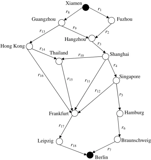
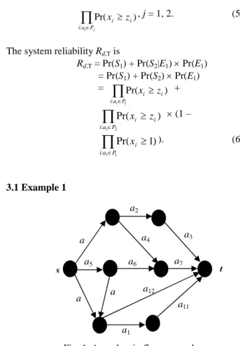
A LCD television manufacturer in Taiwan owns an assembly plant at Xiamen in China and focuses on producing the three types of LCD televisions - 42”LCD television, 47”LCD television, and 55”LCD television. The freight delivery from Xiamen to Berlin in Germany is through the logistics network with 18 routes and 10 MPs (see Figure 1). The available capacity data of carriers (i.e., resource) are listed in Table 1. Each carrier owns multiple capacities, 0, 10 TEU, …, 40 TEU with a probability distribution from carriers’database. The dimensions of the 42”, 47”, and 55”LCD televisions are 108.1 × 76.8 × 20, 125.5 × 83.6 × 24.3, and 138.3 × 94.5 × 25.5 (unit: cm), respectively. A TEU with the size, 589.8 × 235.2 × 238.5, can load approximately 200 (resp. 130 and 100) pieces of 42” (resp. 47”and 55”) LCD televisions. In general, one unit of LCD televisions is calculated in terms of 100 pieces. Hence, one unit of 42”(resp. 47”and 55”) LCD televisions consumes approximately 0.5 (resp. 0.8 and 1) TEU, i.e. w1= 0.5 (resp. w2= 0.8 and w3= 1).

Figure 1. A practical logistics network connecting Xiamen and Berlin.

Xiamen

Guangzhou Fuzhou

Hangzhou Thailand

Hong Kong

Shanghai

Singapore

Frankfurt Hamburg

Berlin Leipzig

r₁₄

r10

r15

r16

r4

r12

r11

r8 r1

r₂ r9

r13

r5

r6

r17

r18

r3

r₇

Braunschweig

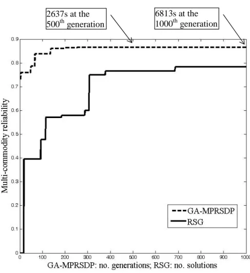
Figure 2. The comparison between GA-MPRSDP and RSG.

The manufacturer has acquired such an order which is to ship 1,000 pieces of 42”LCD television, 2,000 pieces of 47”LCD television, and 2,000 pieces of 55”LCD television to the customer at Berlin, i.e., D = (10, 20, 20). The manufacturer pays close attention to increase the customer’s satisfaction and thus devotes to finding the best carrier selection (i.e., resource allocation).

For the demand D = (10, 20, 20), the manufacturer pays the delivery expanse at most $72,000 USD (United States dollar). For this case, we execute the GA-MPRSDP with θ= 50, α= 0.8, β= 0.05 and λ

= 1000 for 10 times to observe the largest maximal system reliability, the average maximal system reliability, the largest CPU time, and the average CPU time. The experimental result presents the largest maximal system reliability is 0.86618217, the average maximal system reliability is 0.84926714, the largest CPU time is 6813 seconds, and the average CPU time is 5906 seconds. In other words, the addressed problem can be solved by the GA in a reasonable time. Table 2 lists the optimal resource allocation with the largest maximal system reliability. Furthermore, the GA is compared with the random solution generation (RSG) by searching for 1000 solutions, in which the RSG keeps searching for a better solution by randomly producing solutions without any evolution process. Figure 2 summarizes the comparison of the proposed approach and the RSG, and shows that

6813s at the 1000^thgeneration 2637s at the

500^thgeneration

the GA obtains larger maximal system reliability than the RSG.

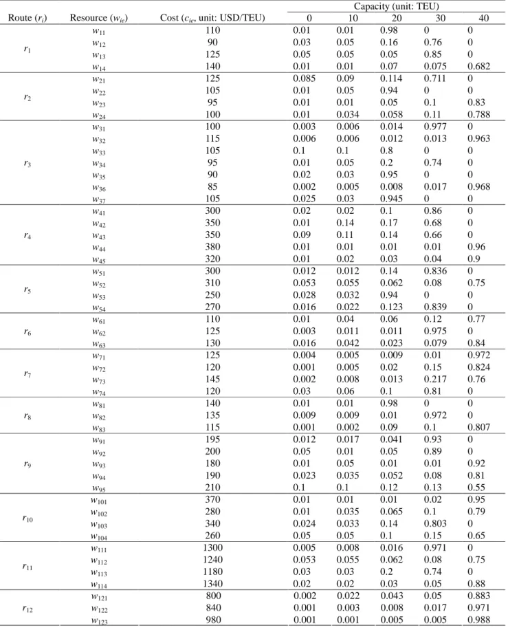
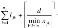
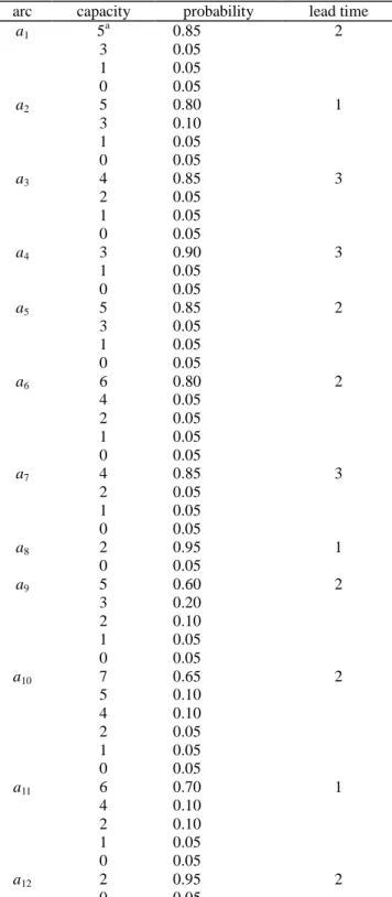
Table 1 The capacities of the resources on routes in Figure 1

Capacity (unit: TEU)

Route (r_i) Resource (w_ie) Cost (c_ie, unit: USD/TEU) 0 10 20 30 40

w₁₁ 110 0.01 0.01 0.98 0 0

w₁₂ 90 0.03 0.05 0.16 0.76 0

w₁₃ 125 0.05 0.05 0.05 0.85 0

r₁

w₁₄ 140 0.01 0.01 0.07 0.075 0.682

w₂₁ 125 0.085 0.09 0.114 0.711 0

w₂₂ 105 0.01 0.05 0.94 0 0

w₂₃ 95 0.01 0.01 0.05 0.1 0.83

r₂

w₂₄ 100 0.01 0.034 0.058 0.11 0.788

w31 100 0.003 0.006 0.014 0.977 0

w₃₂ 115 0.006 0.006 0.012 0.013 0.963

w33 105 0.1 0.1 0.8 0 0

w₃₄ 95 0.01 0.05 0.2 0.74 0

w35 90 0.02 0.03 0.95 0 0

w₃₆ 85 0.002 0.005 0.008 0.017 0.968

r₃

w37 105 0.025 0.03 0.945 0 0

w₄₁ 300 0.02 0.02 0.1 0.86 0

w42 350 0.01 0.14 0.17 0.68 0

w₄₃ 350 0.09 0.11 0.14 0.66 0

w44 380 0.01 0.01 0.01 0.01 0.96

r₄

w₄₅ 320 0.01 0.02 0.03 0.04 0.9

w₅₁ 300 0.012 0.012 0.14 0.836 0

w₅₂ 310 0.053 0.055 0.062 0.08 0.75

w53 250 0.028 0.032 0.94 0 0

r5

w₅₄ 270 0.016 0.022 0.123 0.839 0

w₆₁ 110 0.01 0.04 0.06 0.12 0.77

w₆₂ 125 0.003 0.011 0.011 0.975 0

r₆

w₆₃ 130 0.016 0.042 0.023 0.079 0.84

w₇₁ 125 0.004 0.005 0.009 0.01 0.972

w₇₂ 120 0.001 0.005 0.02 0.15 0.824

w₇₃ 145 0.002 0.008 0.013 0.217 0.76

r₇

w₇₄ 120 0.03 0.06 0.1 0.81 0

w81 140 0.01 0.01 0.98 0 0

w₈₂ 135 0.009 0.009 0.01 0.972 0

r8

w₈₃ 115 0.001 0.002 0.09 0.1 0.807

w₉₁ 195 0.012 0.017 0.041 0.93 0

w92 200 0.05 0.01 0.05 0.89 0

w₉₃ 180 0.01 0.05 0.01 0.01 0.92

w94 190 0.023 0.035 0.052 0.08 0.81

r9

w₉₅ 210 0.1 0.1 0.12 0.13 0.55

w101 370 0.01 0.01 0.01 0.02 0.95

w₁₀₂ 280 0.01 0.035 0.065 0.1 0.79

w103 340 0.024 0.033 0.14 0.803 0

r₁₀

w₁₀₄ 260 0.05 0.05 0.1 0.15 0.65

w111 1300 0.005 0.008 0.016 0.971 0

w₁₁₂ 1240 0.053 0.055 0.062 0.08 0.75

w₁₁₃ 1180 0.03 0.03 0.2 0.74 0

r11

w₁₁₄ 1340 0.02 0.02 0.03 0.05 0.88

w₁₂₁ 800 0.002 0.022 0.043 0.05 0.883

w₁₂₂ 840 0.001 0.003 0.008 0.017 0.971

r₁₂

w₁₂₃ 980 0.001 0.001 0.005 0.005 0.988

w131 70 0.012 0.012 0.14 0.17 0.666

w₁₃₂ 60 0.053 0.055 0.062 0.08 0.75

w133 85 0.028 0.032 0.94 0 0

w₁₃₄ 75 0.016 0.022 0.123 0.839 0

w135 80 0.004 0.008 0.009 0.979 0

w₁₃₆ 90 0.01 0.01 0.025 0.03 0.925

r13

w137 100 0.001 0.006 0.007 0.009 0.977

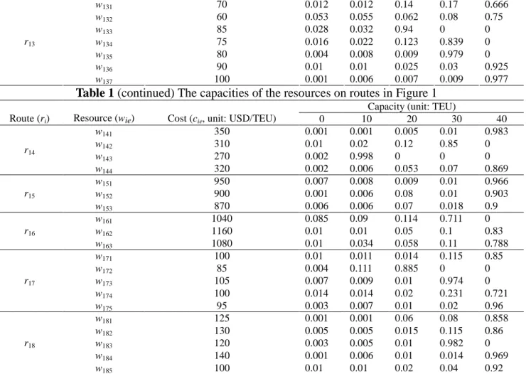
Table 1 (continued) The capacities of the resources on routes in Figure 1

Capacity (unit: TEU)

Route (r_i) Resource (w_ie) Cost (c_ie, unit: USD/TEU) 0 10 20 30 40

w₁₄₁ 350 0.001 0.001 0.005 0.01 0.983

w142 310 0.01 0.02 0.12 0.85 0

w₁₄₃ 270 0.002 0.998 0 0 0

r₁₄

w144 320 0.002 0.006 0.053 0.07 0.869

w₁₅₁ 950 0.007 0.008 0.009 0.01 0.966

w₁₅₂ 900 0.001 0.006 0.08 0.01 0.903

r₁₅

w₁₅₃ 870 0.006 0.006 0.07 0.018 0.9

w161 1040 0.085 0.09 0.114 0.711 0

w₁₆₂ 1160 0.01 0.01 0.05 0.1 0.83

r₁₆

w₁₆₃ 1080 0.01 0.034 0.058 0.11 0.788

w₁₇₁ 100 0.01 0.011 0.014 0.115 0.85

w₁₇₂ 85 0.004 0.111 0.885 0 0

w₁₇₃ 105 0.007 0.009 0.01 0.974 0

w₁₇₄ 100 0.014 0.014 0.02 0.231 0.721

r₁₇

w₁₇₅ 95 0.003 0.007 0.01 0.02 0.96

w₁₈₁ 125 0.001 0.001 0.06 0.08 0.858

w₁₈₂ 130 0.005 0.005 0.015 0.115 0.86

w₁₈₃ 120 0.003 0.005 0.01 0.982 0

w₁₈₄ 140 0.001 0.006 0.01 0.014 0.969

r18

w₁₈₅ 100 0.01 0.01 0.02 0.04 0.92

Table 2 The optimal resource allocation of Figure 1

Maximal system reliability: 0.86618217

i of r_i Selected resource: e of w_ie i of r_i Selected resource: e of w_ie

1 4 ¹⁰ 2

2 3 ¹¹ 3

3 6 ¹² 1

4 5 ¹³ 7

5 1 ¹⁴ 2

6 2 ¹⁵ 3

7 2 ¹⁶ 3

8 3 ¹⁷ 5

9 3 ¹⁸ 3

2. Conclusion and discussion

In the above case, although the logistics networks are not very complex, the number of possible resource allocations is

18 i i

z 



121,927,680,000. That is, it is very time-consuming by using the implicit enumeration approach to solve such a problem as the logistics network is rather complicated.

The GA based approach integrating the MPs and the RSDP is proposed to solve the addressed problem.

For the practical case with D = (10, 20, 20) and C = 72,000, the optimal carrier selection can be found in 6813 seconds by the proposed approach. Moreover, it finds better solutions than the RSG. In addition, the proposed approach is not only applied to the case of multi-commodity shipment but also applied to the case of single-commodity shipment.

參考文獻

[1] K.K. Aggarwal, J.S. Gupta, K.B. Misra, A simple method for reliability evaluation of a communication system, IEEE Transactions on Communications 23 (1975) 563-565.

[2] G. Arnoldsson, Optimal allocation for linear combinations of linear predictors in generalized linear models, Journal of Applied Statistics 23(1996) 493-505.

[3] G. Levitin, Redundancy optimization for multi-state system with fixed resource-requirements and unreliable sources, IEEE Transactions on Reliability 50(2001) 52-87.

[4] G. Levitin, Reliability evaluation for acyclic consecutively connected networks with multistate elements, Reliability Engineering and System Safety 73 (2001) 137-143.

[5] G. Levitin and A. Lisnianski, Reliability optimization for weighted voting system, Reliability Engineering and System Safety 71 (2001) 131-138.

[6] G. Levitin and A. Lisnianski, Structure optimization of multi-state system with two failure modes, Reliability Engineering and System Safety 72 (2001) 75-89.

[7] G. Levitin, Optimal allocation of elements in a linear multi-state sliding window system, Reliability Engineering and System Safety 76 (2002) 245-254.

[8] G. Levitin, Optimal reliability enhancement for multi-state transmission networks with fixed transmission times, Reliability Engineering & System Safety 76 (2002) 287-299.

[9] C.C. Jane, J.S. Lin, J. Yuan, On reliability evaluation of a limited-flow network in terms of minimal cutsets, IEEE Transactions on Reliability 42 (1993) 354-361.

[10] J.S. Lin, C.C. Jane, J. Yuan, On reliability evaluation of a capacitated-flow network in terms of minimal pathsets, Networks 25 (1995) 131-138.

[11] J.S. Lin, Reliability evaluation of capacitated-flow networks with budget constraints, IIE Transactions 30 (1998) 1175-1180.

[12] Y.K. Lin, On Reliability evaluation of a stochastic-flow network in terms of minimal cuts, Journal of Chinese Institute of Industrial Engineers 18 (2001) 49-54.

[13] Y.K. Lin, Study on the multicommodity reliability of a capacitated-flow network, Computers &

Mathematics with Applications 42 (2001) 255-264.

[2] Y.K. Lin, A simple algorithm for reliability evaluation of a stochastic-flow network with node failure, Computers and Operations Research 28 (2001) 1277-1285.

[14] Y.K. Lin, Using minimal cuts to evaluate the system reliability of a stochastic-flow network with failures at nodes and arcs, Reliability Engineering & System Safety 75 (2002) 41 –46.

[15] Y.K. Lin, On the multicommodity reliability for a stochastic- flow network with node failure under budget constraint, Journal of Chinese Institute of Industrial Engineers 20 (2003) 42–48.

[16] Y.K. Lin, Reliability evaluation for a multi-commodity flow model under budget constraint, Journal of the Chinese Institute of Engineers 25 (2002) 109- 116.

[17] Y.K. Lin, Reliability of a stochastic-flow network with unreliable branches & nodes under budget constraints. IEEE Transactions on Reliability 53 (2004) 381-387.

[18] Y.K. Lin, “Evaluatetheperformanceofastochastic-flow network with cost attribute in terms of minimalcuts”,Reliability Engineering & System Safety. 91 (2006) 539-545.

[19] Y.K. Lin, A simple algorithm to generate all (d,B)-MCs of a multicommodity stochastic-flow network”,Reliability Engineering & System Safety. 91 (2006) 923-929.

[20] J. Xue, On multistate system analysis, IEEE Transactions on Reliability 34 (1985) 329-337.

[21] W.C. Yeh, A revised layered-network algorithm to search for all d-minpaths of a limited-flow acyclic network, IEEE Transactions on Reliability 47 (1998) 436-442.

[22] W.C. Yeh, A simple algorithm to search for all d-MPs with unreliable nodes, Reliability Engineering & System Safety 73 (2001) 49-54.

[23] W.C. Yeh, A simple approach to search for all d-MCs of a limited-flow network, Reliability Engineering & System Safety 71 (2001) 15-19.

[24] W.C. Yeh, A new approach to evaluate reliability of multistate networks under the cost constraint.

Omega 33 (2005) 203-209.

國科會補助專題研究計畫成果報告自評表

請就研究內容與原計畫相符程度、達成預期目標情況、研究成果之學術或應用價值

（簡要敘述成果所代表之意義、價值、影響或進一步發展之可能性）、是否適合在 學術期刊發表或申請專利、主要發現或其他有關價值等，作一綜合評估。

1. 請就研究內容與原計畫相符程度、達成預期目標情況作一綜合評估

■ 達成目標

□ 未達成目標（請說明，以 100 字為限）

□ 實驗失敗

□ 因故實驗中斷

□ 其他原因 說明：

2. 研究成果在學術期刊發表或申請專利等情形：

論文：■已發表 □未發表之文稿 □撰寫中 □無 專利：□已獲得 ■申請中 □無

技轉：□已技轉 □洽談中 □無 其他：（以 100 字為限）

3. 請依學術成就、技術創新、社會影響等方面，評估研究成果之學術或應用價值

（簡要敘述成果所代表之意義、價值、影響或進一步發展之可能性） （以 500 字 為限）

1. 就學術上貢獻而言，將使隨機性流量網路可同時考量「最佳化配置」、「傳輸成本」、「傳輸

商品種類多寡」、「容量」與「失效節點」等因素的影響。不僅使流量網路之理論更臻完整，

所提出的網路模型能擴大作業研究領域，激發更多學者參與此一領域之研究。可將成果投 稿於國際上關於可靠度、品質或 OR 領域之 SCI 學術期刊。

2. 於實務上貢獻而言，我們提出相當完整的網路模型，可視為工具箱，遇到實際系統可以採

用不同的模型以真實反應該系統的特色。

3. 就人員訓練方面，能夠以紮實嚴謹的過程處理流量網路問題，並且能結合網路分析理論、

柔性運算、線性代數、作業研究與統計理論。並培養以數理能力分析演算法之時間複雜度，

以及以模擬方法分析演算法之時間複雜度。

4. 有助於品管、可靠度工程及維護度工程的研究工作，故可藉此培養出一些可靠度及維護度

工程的人才。

國科會補助計畫衍生研發成果推廣資料表

日期：98 年 8 月 27 日

國科會補助計畫

計畫名稱：可靠度導向之隨機流量網路最佳化資源配置研究 計畫主持人：林義貴

計畫編號：NSC 96-2628-E-011-116-MY 領域：

（中文）最佳可靠度之隨機物流網路運輸商選擇方法

研發成果名稱

（英文）The method of carrier selection for stochastic logistics network with optimal reliability

成果歸屬機構

^{台灣科技大學}

發明人

(創作人)

林義貴、葉承達

（中文）本技術主要用以搜尋最佳的資源配置，使得系統可靠度 最佳，並且該技術了結合了基因演算法、最小路徑之網路特性以 及遞迴不交合法。在本技術中，基因演算法主要用以搜尋最佳的 資源配置方式，而最小路徑與遞迴不交合法則是用以計算一組資 源配置下的系統可靠度，其主要是利用最小路徑之網路特性，找 出所有滿足特定需求量的下界負載向量，並將系統可靠度表示為 這些向量的聯集形式，最後利用遞迴不交合法計算該集合之機 率，即系統可靠度。本技術不僅可以有效處理單一型態資源的配 置，亦可處理兩種型態資源的配置。

技術說明

（英文）The technology integrates the genetic algorithm, minimal paths and Recursive Sum of Disjoint Products (RSDP) and determines the optimal resource allocation with the maximal network reliability.

In his technology, the GA is developed to search for the optimal resource allocation, the minimal paths and the RSDP is utilized to evaluate the system reliability associated with a resource allocation.

The minimal capacity vectors for a given demand are found in terms of the minimal paths and then the system reliability is represented as the form of the union set by using these vectors. Finally, the RSDP is utilized to calculate the probability of the set. The technology can not only deal with the single-type resource allocation but also the double-resource allocation.

產業別

電腦及周邊產業、運輸工具產業、電力供應產業、顧問諮詢業

技術/產品應用範圍

任何電腦電子產品，若需評估物流網路由供應商配送到顧客端之 需求，皆可在該電子產品上附加此功能

技術移轉可行性及預期 效益

全球化影響下，製造業外移，商品往往需經由物流網路配送至顧 客端上，而商品是否能成功的配送至顧客端則為重要的顧客滿意 度指標之一，本創作即提供一套如何以可靠度為基礎選擇物流網 路上的最佳運輸商組合之技術

註：本項研發成果若尚未申請專利，請勿揭露可申請專利之主要內容。

國科會補助專題研究計畫項下出席國際學術會議心得報告

日期：98 年 8 月 18 日

報告人姓名 林義貴 服務機構

及職稱

國立台灣科技大學工業管理系 教授 時間

會議 地點

98 年 8/6-8/8

美國加州舊金山市 本會核定

補助文號

國科會補助專題研究計畫 NSC96-2628-E-011-116-MY3 會議

名稱

(中文): 第十五屆國際科學與應用科技學會可靠度與品質設計國際會議

(英文): Fifteenth ISSAT International Conference on Reliability and Quality in Design 發表

論文 題目

(中文) 隨機流量網路之路由政策問題

（英文）: The routing policy problem of a stochastic flow network

報告內容應包括下列各項：

一、參加會議經過

本次國際會議名稱為『Fifteenth ISSAT International Conference on Reliability and Quality in Design』，由 ISSAT（International Society of Science and Applied Technology）主辦，為期三天（八 月六號至八號地點為美國加州舊金山市。大會主席為美國 Rutgers 大學的 Hoang Pham。本人有 二篇論文於本次會議中發表，排定於第三天中午 session 22 中發表，本人論文主題為隨機流量網 路之路由政策問題，另一篇論文與博士班學生合著，由該生負責口頭報告。會議之前大會主席 Hoang Pham 教授已商請本人擔任下一年度之議程主席，該人事訊息也在大會中宣布。本人除負 責台灣地區的論文投稿及審查過程外，更承擔整個研討會的議程規劃。大會主席與議程主席以 及本人則連續三天商議明年度的議程規劃，並且研擬最佳論文獎與學生論文獎的選拔事宜，將 在會後先篩選出第一波名單，再交由幾位主席評分候選定論文獎得主。大會最後宣佈明年研討 會的舉辦地點為美國華盛頓特區。此次會議中有來自於台灣、美國、日本、韓國、中國、新加 坡、香港等國的學者參加。

二、與會心得

會議中與休息時間與多位美國及中國學者交流目前發展趨勢及教學心得，獲益良多。觀看國外 大師的論文發表台風以及提綱挈領的演講方式，相當值得學習。參與的人數中可發現亞洲地區 以日本最具代表，其次是中國，尤其有許多的美國學者來自於中國，形成一股龐大的勢力，相 對而言台灣參與人數增加幅度相當小。有不少教師已經繳交註冊費，卻礙於遠程旅費的關係或 者擔憂 H1N1 的威脅而紛紛缺席，殊為可惜。

三、考察參觀活動(無是項活動者省略) 四、建議

未來可以集中國內學者火力爭取於國內舉辦此重要之國際盛事，尤其鄰近的日本及新加坡皆表 達出主辦此校國際會議的高度意願，國內學者更應積極面對之。同時國內重點大學不僅應培養 此企圖心，更應在硬體設施上建構一可辦國際會議之演講廳，至於 session 可在一般教室舉辦。

五、攜回資料名稱及內容

攜回本次大會的論文集、議程冊及一些相關會議之 call papers。包括

1. 15th ISSAT International Conference on Reliability and Quality in Design 研討會論文集 2. 16th ISSAT International Conference on Reliability and Quality in Design, August 5-7, 2010,

Washington, DC, USA, Call for Papers.

六、其他

國科會補助專題研究計畫項下出席國際學術會議心得報告

99 年 2 月 3 日

報告人姓名 林義貴 服務機構

及職稱

國立台灣科技大學工業管理系 教授 時間

會議 地點

99 年 1 月 25 日起 99 年 1 月 28 日止

泰國曼谷

本會核定 補助文號

國科會補助專題研究計畫 NSC96-2628-E-011-116-MY3 會議

名稱

(中文): 第 2 屆產業與管理教育國際研討會

(英文): 2^ndInternational Conference on Business & Management Education 發表

論文 題目

(中文) 本次並未發表論文

（英文）:

報告內容應包括下列各項：

七、參加會議經過

本次國際會議名稱為『2^ndInternational Conference on Business & Management Education』，由泰 國之大學University of Balamand與紐西蘭的大學Eastern Institute of Technology主辦，為期4天（1 月25號至28號）地點為泰國首都曼谷市的飯店Ramada D'MA Hotel。本人對於討論議題中的

「Business Systems and Architecture」（一月26日的下午）、「Learning and Knowledge Production」

（一月26日的下午）、「Asian Business Issues」（一月27日的下午）、「Human Resources Management」

（一月27日的下午）、與「Current Business & Management Issues」（1月28日上午）的幾項議題 很有興趣，分別聆聽這些討論場次的幾篇論文聆聽。此次會議中有來自於馬來西亞、印尼、印 度、伊朗、澳洲、南韓、台灣、美國、以色列、英國、中國、新加坡、日本、埃及、紐西蘭等 國的學者參加。

八、與會心得

會議中與休息時間與多位馬來西亞與印尼學者交流目前發展趨勢及教學心得，獲益良多。尤其 牽涉到 MBA 的教育，特別是針對 EMBA 的部分，本系屬於管理學院，亦招收許多的 EMBA 學 生，雖然有很豐富的業界經驗，但是牽涉到研究議題的時候卻難有紮實的研究，主要便在於雙 方認知的差異。如何透過業界豐富的經驗，將學界的研究更務實化，也是各個國家在管理領域 遇到的相同問題。針對這一問題，我們的共識為透過 EMBA 學生與日間部學生的配合共同完成 論文，可以讓一般的研究更為深入且讓實務的問題進入學界的課題中。從中的討論也發現工管 的一些績效分析模型較少使用於管理領域，例如人員的績效評估尚未有人利用網路的方式求 解，目前大多的學者聯想到的為 ANP(分析網路法)，但這一方法乃是針對方案以及準則進行評 估，並非直接進行績效評估。

九、考察參觀活動(無是項活動者省略) 十、建議

這些會議的參與者來自許多東南亞國家，這些國家的經濟皆為起步且有不錯的前景，相信爾後 若舉辦類似的會議，可以奠立台灣在亞洲區的學界領導位階，不妨在策略上可以逐漸將亞洲列 為學術影響力的重心。

十一、 攜回資料名稱及內容

攜回本次大會的論文集、議程冊及一些相關會議之 call papers。

十二、 其他