生物晶片資料分析與肺腺癌存活之預測

(1)

國立臺灣大學理學院數學系碩士論文

Department of Mathematics College of Science National Taiwan University

Master Thesis

生物晶片資料分析與肺腺癌存活之預測 Microarray Data Analysis and

Prognosis of Lung Adenocarcinomas

何昊 Hao Ho

指導教授: 李克昭教授 Advisor: Professor Ker-Chau Li

中華民國九十九年二月 February 2010

(2)

i

誌謝

七年前，第一次走進台大數學系。一轉眼七年過去了，也將正式離開這充滿回憶的地方。在這裡，我度過了大半的青春時光，失去了很多，得到了更多。所有好的、不好的，開心、不開心的，都將化成我最珍貴的回憶。

首先要感謝的是養我育我、對我萬般包容的家人。感謝爸爸、媽媽無論何時何地都給予我最大的支持。感謝爺爺、奶奶在我小的時候對我的照顧及教育。感謝所有無論住在一起或沒住在一起，一直關心我的家人。請原諒我的不開朗以及任性。我愛你們，謝謝你們給了我一切最好的。

感謝李克昭老師的指導，寬廣了我的視野，更見識到問問題的藝術。感謝老師您給我如此大的空間獨立地思考、學習、研究，又總在關鍵時候指導我什麼才是真正最重要的，讓我不會迷失在自己絮亂的想法之中。感謝陳宏老師，因為您的啟蒙，讓我決定走上統計這條路。感謝江金倉老師亦師亦友

、直言不諱的給予當頭棒喝以及鼓勵。感謝陳素雲老師不厭其煩的提點，無論在統計以及英文寫作上都讓我獲益良多。感謝簫朱杏老師在我的研究過程中給予的所有幫助。感謝袁新盛老師耐心的陪我討論我那多且煩雜的問題。

感謝所有曾在我的世界中留下不同軌跡的朋友們。感謝你們給了我另一份歸屬感。感謝數學系的大伙兒、天外天的兄弟們、ＭＩＢ的同伴們、替代役的長官及夥伴們、歷任資Ａ資Ｂ的家庭成員們，還有所有關心我以及曾關心我的知己們，謝謝你們帶給我生命中不同的美麗風景。感謝我最愛的妳，

陪我走過這十年的求學生涯。感謝妳的好，讓我成長。一路上要感謝的人實在太多，然而，誌謝可用的篇幅又太少，請原諒我無法將心中所有的感謝在此一一訴盡。

最後，僅將所有的感謝化成兩個字，再一次的向你們說：謝謝！

(3)

ii

中文摘要

近年來肺癌高居國內及全球癌症相關死因首位，其死亡率至今仍然居高不下。非小細胞肺癌乃發生率最高之肺癌，其中又以肺腺癌最為普遍。研究指出，肺癌病患的治療方式不只取決於腫瘤類型，而不同肺癌分期亦應適當選擇給予不同治療方式。因此，為幫助病患選取最有利之治療方式，建立更準確之新肺癌診斷方法，有其重要性及迫切性。其中，因前期肺癌病患仍有數種治療方式可選擇，故對於前期肺癌病患之診斷最為重要。

生物晶片技術的發展使得研究人員得以同步測量數以萬計之基因表現量，

並提供了新的研究平台。一項大型的肺腺癌研究建立了豐富的肺腺癌病患之基因表現量資料和臨床資料，用以建立及驗證數種以基因表現量導出之肺癌診斷方法。然而，對於前期病患的存活預測，尚未能找到一種基因訊號對於所有的驗證資料皆能達到百分之五之顯著水準。我們的研究目的即是重新研究這份資料，以期建立一個新的基因訊號對於所有的驗證資料皆能有顯著的存活預測力。

我們引用一個兩階段之維度縮減方法佐以部份的修正來導出肺癌診斷之基因訊號。在第一階段中，我們以基因和存活時間的相關性與配對基因和存活時間的流動關聯性來選出重要的候選基因。第二階段，我們則使用了改良的切片逆迴歸分析方法導出最後的肺癌診斷基因訊號。

分析結果指出，以相同的驗證流程檢驗我們導出的基因訊號，在所有的驗證資料都能達到百分之五之顯著水準的存活預測能力，更進一步的，在另一個包含肺腺癌及鱗狀細胞癌的非小細胞肺癌資料上，我們導出的基因訊號也同樣達到百分之五之顯著水準的存活預測能力。因此，我們認為以TMEM 66，CSRP1，BECN1，FOSL2，ERO1L，SRP54及PAWR七個基因所導出的基因訊號對於非小細胞肺癌病患有好的存活預測能力。

(4)

iii

Abstract

Purpose Recently, several new gene expressions based signatures were pro- posed to predictive the survival of Non Small Cell Lung Cancer (NSCLC) patients. However, for stage I patients, the task is more difficult and no signatures had been found from a large study of lung adenocarcinoma. We reanalyzed this large sample data and tried to construct a gene signature, which had significant prediction power for all stage and early stage patients in all the validation sets. We also used an external independent cohort data set containing both adenocarcinomas and squamous cell carcinomas to test if our gene signature still had significant prediction power for all stage and early stage NSCLC patients.

Materials A total of 442 lung adenocarcinoma gene expression proﬁles from Shedden et al. (2008) containing four independent data sets were reanalyzed in our study. Two of the data sets were combined as a training data set to derive our gene signature. The other two data sets were used for validation.

An external NSCLC data from Duke lung caner cohort was used for addi- tional validation.

Methods We modified a two-steps dimension reduction method proposed by Wu et al. (2008) to derive our gene signature. In the first step, both correlation and liquid association methods were used to select the candidate genes. In the second step, we applied the modified sliced inverse regression proposed by Li et al. (1998) to derive a gene signature from the candidate genes.

Results Five genes TMEM66, CSRP1, BECN1, FOSL2 and ERO1L were selected by correlation methods. SRP54 and PAWR (as a LA pair) were selected by liquid association method. The ﬁnal signature gave signiﬁcant

(5)

iv prediction power for samples with all stage patients and for samples with stage I patients only in all the validation sets.

Conclusion The gene signature derived from the seven genes (TMEM66, CSRP1, BECN1, FOSL2, ERO1L, SRP54 and PAWR) had good prediction power for all stage and early stage NSCLC patients.

(6)

List of Figures

2.1 The ﬂow chart of analysis procedures. . . 10 3.1 Scatter plots of gene expression proﬁles of DDR1 in HLM and

UM two data sets preprocessed together versus preprocessed separately by dChip algorithm: The left panel is log-2 transformed gene expression proﬁles and the right panel is normal quantile transformed gene expression proﬁles. . . 12 3.2 Histogram of the ranks of mean expressions of 22,215 probe

sets in training data set after excluded inconsistent genes. . . 15 3.3 Histogram of the ranks of mean expression proﬁles of the re-

maining genes with a total of 22,215 probe sets in training data set. . . 16 4.1 The log-log Kaplan-Meier curves of diﬀerent stages for the

training data set. . . 21 4.2 Observed Kaplan-Meier plot and Cox proportional hazard

model. Cox coeﬀicients of (Stage IB, II, III/IV)= (0.50, 1.05, 1.81). The hazard ratio of (Stage IB, II, III/IV)= (1.64, 2.85, 6.12). . . 22

vii

(9)

LIST OF FIGURES viii 4.3 The scatter plot of ratios of expected number to the observed

number versus cutoﬀs of the absolute value of correlation co- eﬀicient in the training data. . . 27 4.4 The scatter plot of ratios of expected number to the observed

number versus cutoﬀs of the absolute value of correlation co- eﬀicient in one of the 1,000 permutations. . . 28 4.5 The scatter plot of ratios of expected number to the observed

number versus cutoﬀs of the absolute value of LA scores in the training data. . . 35 5.1 Kaplan-Meier survival curves for all stage and stage I samples

in training data set separated by gene signature constructed by only ﬁve correlation genes. . . 44 5.2 Kaplan-Meier survival curves for all stage samples in training

data separated by gene signature constructed by ﬁve correlation genes and one LA pair. . . 45 5.3 Kaplan-Meier survival curves for stage I samples in training

data separated by gene signature constructed by ﬁve correlation genes and one LA pair. . . 46 6.1 Kaplan-Meier curves for all stage samples separated by gene

signature . . . 55 6.2 Kaplan-Meier curves for stage I samples separated by gene

signature . . . 56 6.3 Kaplan-Meier curves for all stage samples separated by TNM

stage . . . 57 6.4 Kaplan-Meier curves for stage I samples separated by TNM

stage . . . 58

(10)

LIST OF FIGURES ix 7.1 Kaplan-Meier curves for all stage and stage I samples sepa-

rated by gene signature preprocessed by dChip in CAN/DF and MSK data . . . 67 7.2 Kaplan-Meier curves for all stage and stage I samples sepa-

rated by gene signature preprocessed by RMA in CAN/DF and MSK data . . . 68

(11)

List of Tables

2.1 Summary statistics of the clinical and survival data . . . 5 4.1 Simulation comparison between two imputation methods . . . 25 4.2 The candidate genes and the correlation coeﬀicients of the

candidate genes and the imputed survival time . . . 29 4.3 The LA hub gene SRP54 and its LA paired genes . . . 35 5.1 The estimated coeﬀicients of SIR direction . . . 48 5.2 Hazard ratio with the corresponding 95% conﬁdent interval,

p-value and the CPE of our gene signature . . . 48 5.3 Hazard ratios with the corresponding 95% conﬁdent intervals

and p-values of our gene signature and clinical covariates . . . 49 6.1 Validation results in CAN/DF, MSK and Duke data sets . . . 54 7.1 The estimated coeﬀicients of SIR direction for expression pro-

ﬁles preprocessed by dChip and RMA . . . 65 7.2 Validation results in CAN/DF and MSK data preprocessed

by dChip and RMA . . . 66

x

(12)

Chapter 1 Introduction

In the latest years, lung cancer is the leading cause of caner death in many Western countries and also in Taiwan. The most common cell type of lung cancer is Non Small Cell Lung Cancer (NSCLC), especially the lung adenocarcinomas [1] [2]. The treatment selection of different patients is dependent on various factors including tumor cell types and cancer stages. Recently, the adjuvant chemotherapy has been proved for significantly improving the survival of stage IB and stage II patients [3]. However, for some early stage patients with good prognoses, the benefit is not significant. To help early stage patients select the most beneficial treatment, a new diagnostic method is urgently needed.

The development of microarray technology has helped researchers to measure more than ten thousands of gene expressions simultaneously. From the information contained in these data, several new gene expression based signatures were introduced to predict to survival of NSCLC patients [4]-[9].

However, to reproduce and to validate these signatures in general are not easy. A large sample lung adenocarcinomas data containing four indepen-

1

(13)

CHAPTER 1. INTRODUCTION 2 dent cohort data sets was generated to compare the performance of several latest expression based diagnostic signatures [10]. Nevertheless, the study did not found a signature having signiﬁcant prediction power for samples with stage I patients only in all the validation data sets.

We reanalyzed this large adenocarcinomas data starting from data preprocessing to filter out some non-informative genes. A two-steps dimension reduction method proposed by Wu et al. (2008) [11] was then applied with some modifications for deriving diagnostic signature on the training set. In the first step, both correlation and liquid association methods [13] [14] were used to select the candidate genes. In the second step, we applied the mod- ified sliced inverse regression proposed by Li et al. (1998) [16] to derive the signature from the candidate genes. Based on the same validation procedure for all the testing data as in Shedden et al. (2008), our signature gave signif- icant prediction power for samples with all stage patients and samples with stage I patients only. Furthermore, we also used an external independent cohort data set containing both adenocarcinomas and squamous cell carcinomas to test if our gene signature still had significant prediction power for all stage and early stage patients. Our gene signature still gave significant prediction power in this validation data set.

Here we summarize the main contents of this thesis. We introduce all the cohort data sets used in our analysis and our analysis procedure in Chapter 2. Three diﬀerent criterions for gene ﬁltering are introduced in Chapter 3.

In Chapter 4, we introduce how we select the candidate genes by correlation and liquid association (LA) methods. A modiﬁed imputation method for censored data is also given. In Chapter 5, we discuss how we derived the

(14)

CHAPTER 1. INTRODUCTION 3 gene signature from the selected candidate genes. A brief introduction for modified sliced inverse regression and its implementation is also given. The validation results and cross platform adjustment for testing sets are presented in Chapter 6. In Chapter 7, we discuss the genes we used in our signature, the relationship between our permutation procedure and Benjamini-Hochberg procedure under independent assumption in our data setting, and the effect, which might be caused by different preprocessing methods.

(15)

Chapter 2 Materials and analysis procedure

2.1 Materials

In this section, we introduce several independent cohort data sets we used to construct our gene signature or to test the prediction power of our gene signature. Each data set contains gene expression proﬁles measured by Aﬀymetrix microarray and survival outcome data of Non Small Cell Lung Cancer (NSCLC) patients. Some relevant clinical and pathological data, such as sex, age, TNM tumor stage and tumor cell type are also available. The summary statistics of clinical variables in each data set are given as table 2.1.

442 lung adenocarcinoma data from Shedden et al. (2008)

In Shedden et al. (2008), a large lung adenocarcinomas microarray data was generated from four institutions, Moﬀitt Cancer Center (HLM), Univer- sity of Michigan Cancer Center (UM), Dana-Farber Cancer Institute (CAN/DF)

4

(16)

CHAPTER 2. MATERIALS AND ANALYSIS PROCEDURE 5

Table 2.1: Summary statistics of the clinical and survival data

HLM UM CAN/DF MSK Duke

Sample size 79 177 82 104 111

Age (mean) 67 64 61 65 65

Cell type (% adenocarcinomas) 100% 100% 100% 100% 52%

Sex (% male) 51% 56% 56% 36% 57%

Stage IA 11% 39% 13% 26% 36%

Stage IB 43% 27% 55% 35% 24%

Stage II 27% 16% 32% 19% 16%

Stage III 19% 18% 0% 20% 20%

Stage IV 0% 0% 0% 0% 4%

Median follow up (months) 39 54 51 43 31

Number of deaths 60 102 35 39 58

and the Memorial Sloan-Kettering Cancer Center (MSK), using a common platform, Aﬀymetrix U133A. After excluding samples with poor quality of microarray data or incomplete clinical data, a total of 442 samples from four independent data sets were analyzed in their study. They analyzed the data for validating the following four hypotheses: (1) can gene expression predict the survival of all stage patients? (2) Can gene expression predict the survival of stage I patients? (3) Can gene expression with clinical covariates (stage, sex and age) predict the survival of all stage patients? (4) Can gene expression with clinical covariates predict the survival of stage I patients?

They combined the ﬁrst two data sets, HLM and UM, as a training data set to construct the gene signature, and used the rest two independent data sets,

(17)

CHAPTER 2. MATERIALS AND ANALYSIS PROCEDURE 6 CAN/DF and MSK, to test the prediction power of the derived signatures.

In their reports, with the clinical covariates, several methods gave significant prediction power for all stage and stage I patients in the rest two validation sets, CAN/DF and MSK. However, without clinical covariates, there were no signatures found with significant prediction power for stage I patients in both validation sets. Therefore, in our analysis, we focused on the first and the second hypotheses. Our purpose was to derive a gene signature from the training data set which had significant prediction power for all stage and stage I patients in both validation data sets. The raw data were downloaded from https://caarraydb.nci.nih.gov/caarray/publicExperimentDetailAction.do?ex pId=1015945236141280.

111 NSCLC samples from Duke lung caner cohort

Another microarray data set from Duke lung caner cohort containing 111 NSCLC samples was used to test our gene signature. This data set was a more challenging external validation data set. First we noted that it contained patients of two different tumor cell types, adenocarcinomas and squamous cell carcinomas. The prediction power of our gene signature for patients with different tumor cell types can be tested in this validation set. Second, since the gene expression profiles were measured by a different microarray platform Affymetrix HU133plus2, a cross platform adjustment was needed. The detail of our adjustment is discussed in Chapter 6.

(18)

CHAPTER 2. MATERIALS AND ANALYSIS PROCEDURE 7

2.2 Analysis procedure

In this section, we brieﬂy introduce our analysis procedure and the main methods we used to construct our gene signature. The theoretical and implemented details of these methods are given in later chapters.

The major challenge in microarray data analysis is the large dimension- ality. The number of genes (G) is in the range of ten to fifty thousands but the sample size (n) is only about hundreds. To reduce the effect of microar- ray noise, we used three criterions to filter out non-informative genes. We excluded the genes with low expressions, small variation expressions or with inconsistent expressions between three preprocessing methods, the MAS 5.0 Statistical algorithm from Affymatrix (2001) [18], the dChip algorithm from Li and Wong (2001) [19] and the Robust Multi-chip Average (RMA) from Irizarry et al. (2003) [20]. The detail of this part is discussed in Chapter 3.

After gene filtering, we reduced the number of genes (G) to a related smaller number (G^∗), but the true effective dimensions to the survival time might be much smaller. Our strategy was to implement a two-steps dimen- sion reduction method proposed by Wu et al. (2008) with some modifications.

This approach contained gene selection and signature construction two steps.

In the gene selection part, we used both correlation and liquid association methods to select the important candidate genes related to survival time.

Pearson’s correlation coeﬀicient was introduced to measure the strength of linear dependency between two variables. However, the association between gene expressions and patients survival might not be linear and might be more complicated. The liquid association (LA) method was implemented here to explore the interaction of two genes related to the survival time. Due to the

(19)

CHAPTER 2. MATERIALS AND ANALYSIS PROCEDURE 8 data censoring issue, both correlation and liquid association could not be implemented directly. Therefore, we modified a nonparametric imputation method [11] to impute the censored data, then the correlation coefficients could be evaluated by plugging the imputed survival probability. After that, we calculated and ranked the correlation coefficients between gene expressions and the imputed survival probability by the absolute values. Genes in the first few places were selected as candidate genes in this part. We also proposed a permutation procedure to decide how many genes should be selected. For implementing the liquid association (LA) method, our strategy was to select the genes, which recurrently appeared in the first few extreme LA gene pairs. These genes were called the LA hub genes. We selected the LA hub gene and also its paired genes as candidate genes in this part.

We note that the gene expression profiles and the imputed survival probability were normalized by normal quantile transformed in the first two parts, gene filter and the gene selection. The normal quantile transformation is necessary for the liquid association method and makes the procedure robust against the outliers. Both the correlation and liquid association can be com- puted in the website http://kiefer.stat2.sinica.edu.tw/LAP3/index.php. The details of the imputation methods and liquid association method are given in Chapter 4.

In the signature construction part, the candidate genes selected from the previous step were used to derive a gene signature for survival prediction.

First, we applied the modified sliced inverse regression to estimate the effective dimension reduction (e.d.r.) directions and projected the selected gene expression profiles on the e.d.r. space. If there is only one SIR direction, the

(20)

CHAPTER 2. MATERIALS AND ANALYSIS PROCEDURE 9 estimated e.d.r. direction, found significantly by a large sample chi-squared test, we projected the expression profiles on it as our final gene signature.

Otherwise, we could use the projected directions to fit other survival model, for example the multivariate Cox proportional hazard model, and derive the final gene signature. We note that the normal quantile transformation was not used in this part. The regressors (X) in the dimension reduction model were the candidate gene expression profiles transformed by log-2 transformation and centered toward sample mean in training data set. The theoretical derivation and practical implementation of modified sliced inverse regression are given in Chapter 5.

The prediction power of our gene signature was tested in the independent validation data sets. In each validation data set, we used the linear combina- tion coefficients estimated from the training data set to combine the selected gene expressions into a gene signature. We used two ways to present the prediction power of our signature. First we used median of our signatures in each validation set to separate the samples into two groups, high risk and low risk groups, as a categorical classifier. For this categorical classifier, the log rank test was used to test the difference of the survival distribution of two groups. Second, we used our derived gene signature as a continuous risk score to fit the Cox proportional hazard model. We estimated the hazard ratios with corresponding p-value and the concordance probabilities (CPE) [23] for both categorical classifier and the continuous risk score. The CPE estimated the probability that survival outcome agreed with the risk score or categorical classifier under the Cox proportional hazard model. To compare the derived gene signature and the TNM tumor stage the results of multivariate Cox proportional hazard model were also presented. A flow chart of

(21)

CHAPTER 2. MATERIALS AND ANALYSIS PROCEDURE 10 our procedure is given as ﬁgure 2.1.

Training data (HLM+UM)

Gene ﬁlter Inconsistent gene

expressions Low gene

expressions Small varia?on gene expressions

Gene selec?on Correla?on Liquid associa?on

Gene signature construc?on

Modiﬁed sliced inverse regression

(Mul?variate Cox model, if more than one signiﬁcant direc?ons)

Valida?on CAN/DF MSK DUKE

Normal score transforma?on

Log 2 transforma?on

Survival imputa?on

Figure 2.1: The ﬂow chart of analysis procedures.

(22)

Chapter 3 Gene ﬁlter

3.1 Inconsistent gene expressions

At the beginning of microarray analysis, choosing data preprocessing method is still an open issue. MAS 5.0 Statistical algorithm, dChip algorithm and the Robust Multi-chip Average (RMA) method are three widely used data preprocessing methods. However, different methods may lead to different results. In Shedden et al. (2008), they preprocessed the expression profiles by running dChip algorithm on all four data sets together. Never- theless, there was an issue they remarked: running the dChip algorithm on the entire data sets may have removed some of the inter-site differences but is somewhat unrealistic. Figure 3.1 showed a dramatic shift of the data indi- cating that gene expressions preprocessed separately or together as a group using dChip algorithm are not comparably scaled. This inter-site difference may impact the validation results a lot.

In our data analysis, we chose the MAS 5.0 Statistical algorithm for data preprocessing. The MAS 5.0 algorithm allowed us to preprocess the microar-

11

(23)

CHAPTER 3. GENE FILTER 12

10.5 11.0 11.5 12.0

10.511.011.512.0

HLM and UM preprocessed separatly

HLM and UM preprocessed together

UM HLM

-2 -1 0 1 2

-2-1012

HLM and UM preprocessed separatly

HLM and UM preprocessed together

HLM UM

Figure 3.1: Scatter plots of gene expression profiles of DDR1 in HLM and UM two data sets preprocessed together versus preprocessed separately by dChip algorithm: The left panel is log-2 transformed gene expression profiles and the right panel is normal quantile transformed gene expression profiles.

ray data entirely or chip by chip with the same results. However, we thought that the genes with inconsistent expression profiles between three preprocessing methods were unconvinced. Therefore, we filtered out the genes that had inconsistent expression levels between three preprocessing methods. Corre- lation coefficient is a measure also used to measure the similarity of two variables. Here we used it to measure the similarity of the expression levels preprocessed by each two of the three preprocessing methods for each gene.

Nevertheless, since the RMA preprocessed data is in log-2 scale, we may transform it before we calculated the correlation coeﬀicients. Furthermore, the normal quantile transformed correlation coeﬀicients between gene expressions and imputed survival probability is an important selecting criterion in the gene selection part. Thus, we also used the normal quantile transformed

(24)

CHAPTER 3. GENE FILTER 13 correlation coeﬀicient in this part.

Before continuing the introduction of the gene ﬁlter, here we give a def- inition of the normal quantile transformation and note some properties of it.

Deﬁnition 3.1.1. For any n observations x = (x₁, ..., x_n)^′ of variable X, The normal quantile transformation is deﬁne by

N (x) = (

Φ⁻¹( 1 n + 1R₁)

, Φ⁻¹( 1 n + 1R₂)

, ..., Φ⁻¹( 1

n + 1R_n))^′ ,

where Φ(·) is the cumulative distribution function of standard normal distri- bution and R_i is the rank of x_i in x for i = 1, 2, ..., n.

Since Pearson’s correlation coefficient with normal quantile transformation only depends on the rank of observations, it can be viewed as a kind of rank correlation coefficient. It is more robust against outliers than the original Pearson’s correlation coefficient. Furthermore, in elementary statistics, the correlation coefficient between N(x) and x is used to test for the null hy- pothesis that X is normally distributed. The correlation coefficient between N(x) and x is closed to 1 under null hypothesis. If X₁ and X₂ are both normally distributed, the correlation coefficient between N(x₁) and N(x₂) is closed to the correlation coefficient between x1 and x2. Then some properties of the original Pearson’s correlation coefficient carried over. We also note that the normal quantile transformation is necessary for the LA calculation.

Therefore, we used the normal quantile transformed correlation coeﬀicient for all the correlations between two variables in our analysis procedure.

For our real data analysis, ﬁrst we preprocessed the expression proﬁles by using all the three preprocessing methods separately in HLM, UM, CAN/DF

(25)

CHAPTER 3. GENE FILTER 14 and MSK four data sets for three versions of gene expression profiles. Since the CAN/DF and MSK data sets were used for validation, the gene filter was only implemented in the training data sets, HLM and UM. There were 22,215 probe sets on Affymetrix U133A microarray. For each gene in the two training data sets, we evaluated the normal quantile transformed correlation coefficients between each two of the three different preprocessed expression profiles. Thus, there were six correlation coefficients evaluated for each gene.

The genes that had as least one of the six correlation coeﬀicients smaller than 0.78 were excluded.

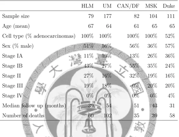
In each data set, the ranks of the mean expressions of the remaining genes with a total of 22,215 probe sets were recorded. The histogram is given in ﬁgure 3.2. In the histogram, the proportion of the remaining genes with high rank is found larger than the proportion of the remaining genes with low rank.

3.2 Low gene expressions

Although microarray can be used to detect more than ten thousands of gene expression profiles simultaneously, the proportion of truly expressed genes might be no greater than half. In this gene filtering part, we evaluated the sample mean expression of each gene in the training set and filtered out the genes with small sample mean expressions. In practice, the genes with sample mean expressions smaller than 300 in the training data set were excluded.

(26)

CHAPTER 3. GENE FILTER 15

HLM

Rank

Frequency

0 5000 10000 15000 20000

020406080100

UM

Rank

Frequency

0 5000 10000 15000 20000

020406080100

CAN/DF

Rank

Frequency

0 5000 10000 15000 20000

020406080100

MSK

Rank

Frequency

0 5000 10000 15000 20000

020406080100

Figure 3.2: Histogram of the ranks of mean expressions of 22,215 probe sets in training data set after excluded inconsistent genes.

3.3 Small variation gene expressions

Another gene filtering criterion we used was the variation of each gene expression profile. Some ”housekeeping” genes expressed constantly high or low for basic reactions. The variations of these gene expression profiles were small and may not relate to the survival time of patients. However, selecting genes by normal quantile transformed correlation coefficients compared the correlations between gene expressions and survival time of patients at the same sale of variation. Some non-informated genes might be selected.

(27)

CHAPTER 3. GENE FILTER 16 Therefore, we excluded the genes with small sample variation of expressions.

In practice, the genes that had standard deviation smaller than 135 in the training data set were excluded.

After three-steps gene filtering, there were 6,252 genes remained in our analysis. The histogram of the ranks of mean expression profiles of the remaining genes with a total of 22,215 probe sets in training data set is given as figure 3.3.

Training data set: inconsistent gene expressions excluded

Rank

Frequency

0 5000 10000 15000 20000

02060100

Training data set: low gene expressions excluded

Rank

Frequency

0 5000 10000 15000 20000

02060100

Training data set: small variation gene expressions excluded

Rank

Frequency

0 5000 10000 15000 20000

02060100

Figure 3.3: Histogram of the ranks of mean expression proﬁles of the remaining genes with a total of 22,215 probe sets in training data set.

(28)

Chapter 4 Gene selection

4.1 Correlation

In the previous chapter, we reduced the number of genes from 22,215 (G) to 6,252 (G^∗) through the three-steps gene ﬁlter. However, the number is still much larger than the sample size 256 (n). The implementation of sliced inverse regression (SIR) requires the covariance matrix Σ_x to be non- singular, which can not hold in such a case. To solve this issue, we used both correlation and liquid association (LA) methods to select the important candidate genes. The genes with greatest correlations to the survival time Y^◦ and gene pairs that had interaction related to the survival time were selected as candidate genes in this part. Due to the censoring of survival data, both correlation and liquid association methods could not be applied directly for the observed time Y = min{Y^◦, C}, where C is the censored time. A modiﬁed imputation method was proposed to impute the survival probability for the censored time, and then both correlation and liquid association methods could be implemented by plugging the imputed survival probability.

17

(29)

CHAPTER 4. GENE SELECTION 18

4.1.1 Imputation of survival time with right censoring

Here we used the normal quantile transformed correlation coefficient described in the previous chapter to measure the correlation between survival time y^◦ and each gene expression profile xg, where g = 1, 2, ..., G^∗. Due to data censoring, we could not use the correlation coefficient between observed time y and gene expression xg. Let δ = 1_{Y◦≤C}(Y^◦, C) be the indicator that indicated the status of each patient. To reduce the effect caused by right censoring, an imputation ˆY^◦ for δ = 0 was needed.

Suppose that Y^◦was the true survival time with survival function S^◦(y^◦) = P (Y^◦ > y^◦) and density function f (y^◦). In elementary statistics, we knew that the conditional mean, E(Y^◦ | Y^◦ > y), minimized the 2-norm impu- tation error loss, l₂( ˆY^◦) = E[( ˆY^◦ − Y^◦)² | Y^◦ > y]. However, Wu et al.

(2008) pointed out the limitation of estimating the conditional mean given that Y^◦ > y by Kaplan-Meier estimate when the last observation was cen- sored in practice. Therefore, we did not adopt the conditional mean. If the 1-norm imputation error loss l₁( ˆY^◦) = E[| ˆY^◦ − Y^◦| | Y^◦ > y] was used, we could impute the censored data by the conditional median given that Y^◦ > y and evaluate the normal quantile transformed correlation coefficient, corr(N (xg), N (ˆy^◦)), to estimate the correlation coefficient between survival time Y^◦ and each gene expression profile X_g.

First we noted that the normal quantile transformation N (·) only de- pended of the ranks of variables. Therefore, it was invariant under any mono- tone transformation, that is N ((h(x₁), h(x₂), ..., h(x_n))^′) = N ((x₁, x₂, ..., x_n)^′) for any monotone function h. Second, the conditional median given that

(30)

CHAPTER 4. GENE SELECTION 19 Y^◦ > y satisﬁed that

S^◦(

median(Y^◦ | Y^◦ > y))

= 1 2S(y).

Furthermore, the distribution function F^◦(·) = 1 − S^◦(·) is a monotone func- tion, so that we have

N (ˆy^◦) = N(

(ˆy^◦₁, ˆy₂^◦, ..., ˆy^◦_n)^′)

= N((

F^◦(ˆy₁^◦), F^◦(ˆy₂^◦), ..., F^◦(ˆy_n^◦))_′)

= N((

1− S^◦(ˆy₁^◦), 1− S^◦(ˆy^◦₂), ..., 1− S^◦(ˆy^◦_n))_′) and

S^◦(ˆy_i^◦) =





S^◦(y_i), if δ_i = 1

1

2S^◦(y_i), if δ_i = 0.

Therefore, instead of estimating the conditional median, we could evaluate the N (ˆy^◦) by plugging the estimated survival function ˆS^◦(·). Wu et al. (2008) proposed a nonparametric imputation procedure by using the Kaplan-Meier estimation for the survival function. The procedure is summarized as the following steps:

Imputation - Kaplan-Meier based

1. Calculate ˆS_i^◦ the Kaplan-Meier estimate of the survival probability;

2. Impute the survival probability by the predicted conditional median

S˜_i^◦ =





Sˆ_i^◦, if δ_i = 1

1

2Sˆ_i^◦, if δ_i = 0;

3. Calculate the percentile ˆp_i = 1− ˜S_i^◦;

4. Calculate the imputed N (ˆy^◦) by performing the normal quantile transformation on ˆp_i.

(31)

CHAPTER 4. GENE SELECTION 20 The implementation of this nonparametric imputation procedure is easy since we only have to calculate the Kaplan-Meier estimate of the survival probability. However, an issue is how we improve the imputation if we have extra information. The TNM tumor stage is strongly related to the survival time of NSCLC patients. It is not suitable to impute the same survival time for diﬀerent stage patients at the same censored time. It motivated us to modify the imputation procedure with this extra information.

Modiﬁed imputation - Cox proportional hazard model based

Previous studies indicated that the survival of NSCLC patients in different TNM tumor stage were significantly different and it motivated us to modify the imputation procedure. Since the original imputation procedure directly followed by the Kaplan-Meier estimate of survival probability, one nature idea was to modify the survival probability estimation by incorpo- rating the TNM tumor stage Z. We assumed that the conditional survival function given Z = z satisfied Cox proportional hazard model.

Cox proportional hazard model is one of the well-known regression sur- vival models. It modeled that the hazard function given Z = z is propor- tional to a baseline hazard function and the logarithm of the ratio is linearly dependent on the regressors,

λ^◦(y^◦ | Z = z) = λ^◦0(y^◦)e^γz.

Here we let Z be a four levels factor which indicated that the patient’s TNM tumor stage is IA, IB, II or III/IV. Then, the relationship between conditional survival function given Z = z and the baseline survival function can be

(32)

50 100 150 200

-2024

Log-Log Survival curve

Figure 4.1: The log-log Kaplan-Meier curves of diﬀerent stages for the training data set.

expressed as

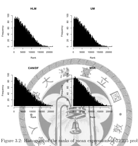
S^◦(Y^◦ | Z = z) = [S0^◦(Y^◦)]ê^γz. (4.1) To check the assumption of Cox proportional hazard model, first we drew the log-log Kaplan-Meier curves of different stages for the training data set.

From the equation (4.1) above, the log-log Kaplan-Meier curves should be parallel if the assumption held. Figure 4.1.1 showed that there was no strong evidence of non-parallelism for our data. Second, we drew the observed versus expected plot for the training data set and it also showed that there was no strong evidence to reject the assumption.

(33)

0 50 100 150

0.00.20.40.60.81.0

Observed and Expected Survival Curve

Figure 4.2: Observed Kaplan-Meier plot and Cox proportional hazard model.

Cox coeﬀicients of (Stage IB, II, III/IV)= (0.50, 1.05, 1.81). The hazard ratio of (Stage IB, II, III/IV)= (1.64, 2.85, 6.12).

Therefore, we assumed that Y^◦ | Z = z satisﬁed the Cox proportional hazard model and imputed the censored time by ˆy^◦ = median(Y^◦ | Y^◦ >

y, Z = z). Then we had

N (ˆy^◦) = N(

(ˆy₁^◦, ˆy^◦₂, ..., ˆy_n^◦)^′)

= N((

1− S0^◦(ˆy^◦₁), 1− S0^◦(ˆy₂^◦), ..., 1− S0^◦(ˆy_n^◦))_′) ,

where S₀^◦(·) was the baseline survival function and it was also a monotone function. Furthermore, we had S₀^◦(ˆy^◦_i) = S₀^◦(yi) if δi = 1 and

S₀^◦(ˆy_i^◦) = (

S^◦(ˆy_i^◦|Z))_exp(γZ)¹

= (1

2S^◦(y_i|Z))_exp(γZ)¹

= (1

2S₀^◦(y_i)^exp(γZ) ) ¹

exp(γZ)

= (1

2)^exp(γZ)¹ S₀^◦(y_i), if δ_i = 0.

(34)

CHAPTER 4. GENE SELECTION 23 From the equations above, we observed that the modified imputation method gave different weights for the censored survival probability of the patients in different stages. In practice, the Cox coefficients γ could be estimated by finding the γ that maximized the partial likelihood. The baseline survival function could be estimated by the Nelson-Allen estimate or Breslow estimate. Then the original procedure could be implemented by replacing the survival probability estimation and the imputed weights. The modified imputation procedure is summarized as the following steps:

1. Estimate the Cox coeﬀicients γ^′s for each TNM tumor stage and the baseline survival probability ˆS_0i^◦;

2. Impute the survival probability by the predicted conditional median

S˜_0i^◦ =





Sˆ_0i^◦, if δ_i = 1 (¹₂)^{exp γzi}¹ Sˆ_0i^◦, if δ_i = 0;

3. Calculate the percentile ˜p_i = 1− ˜S_0i^◦;

4. Calculate the imputed N (ˆy^◦) by performing the normal quantile transformation on ˜p_i.

(35)

4.1.2 A simulation comparison between two imputa- tion methods

To present the improvement of our modiﬁcation, we did a simulation study. First we randomly generated 256 survival time samples from Cox proportional hazard model with a four levels factor regressor. The levels of the factor regressor were uniformly random generated. The baseline survival function was exponential distribution with rate parameter set to be 1 and the Cox coeﬀicients γ’s for each level were set to be (0, 2, 4, 8). Another 256 cen- sored time samples were randomly generated from exponential distribution with rate parameter 3. We set the minimum of the survival time samples and the censoring time samples to be the observed time samples. The average censoring rate was 0.5099.

To assess the performances of the imputation methods, the normal quantile transformed correlation coefficient between true survival time samples and the imputed values, corr(N (y^◦), N (ˆy^◦)), was used to measure the close- ness. For 1,000 simulation runs, we implemented both imputation methods and recorded the correlation coefficients in each run. The average of the correlation coefficients of the Kaplan-Meier based imputation was 0.8684 and the average correlation coefficients of Modified imputation was 0.9096. More- over, there were only three times that the Kaplan-Meier based imputation had correlation coefficient greater than the Modified imputation. We con- cluded that the modified imputation method had better performance when the Cox proportional hazard model assumption held. The results of our simulation were given in the following table.

(36)

Table 4.1: Simulation comparison between two imputation methods Estimated Cox model coeﬀicients Average S.D.

Cox model coefficient ˆγ2 (γ2 = 2) 2.1096 0.6260 Cox model coefficient ˆγ₃ (γ₃ = 4) 4.1355 0.6264 Cox model coefficient ˆγ4 (γ4 = 8) 8.2389 0.7948 Normal quantile transformed correlation coefficient Average S.D.

between true survival time and imputed value

No imputation (Observed time) 0.7786 0.0312

KM based imputation 0.8683 0.0205

Modiﬁed imputation 0.9096 0.0146

Censor rate 0.5099 0.0308

4.1.3 Gene selection in training data by correlation

In this subsection, we presented the results of candidate genes selection by correlation method in the training data set (HLM+UM). For all the samples in the training data set, first we implemented the modified imputation procedure described in the previous subsection to impute the survival probability and performed the normal quantile transformation on the imputed survival probability and each gene expression profile. For each gene, we calculated the correlation coefficient rg between normalized gene expression N (xg) and the imputed N (ˆy^◦) and ranked the 6,252 correlation coefficients by the absolute values. The top five genes with the greatest absolute values of correlation coefficients were selected as our candidate genes. These candidate genes were the only five genes which had the absolute value of correlation coefficients greater than 0.25. The cutoff was determined based on controlling the ratio of the expected number of all true null hypotheses to the real observed

(37)

CHAPTER 4. GENE SELECTION 26 number of correlation coeﬀicients greater than the cutoﬀ

c^∗ = min {

c|[ E[

G^∗

∑

g=1

1(R_g > c)]/[

G^∗

∑

g=1

1(r_g > c)]]

≤ α} ,

where Rg = corr(

N (xg), N (ˆy^◦))

under Xg ⊥ Y^◦ for all g. A permutation procedure was proposed to select the cutoff. For any given cutoff, we estimated the expected number of correlation coefficients greater than the cutoff if survival time was irrelative to all the 6,252 genes by the average of 1,000 runs permutation. The ratio of the expected number to the real observed number of correlation coefficients greater than the cutoff was used to choose the cutoff. The procedure could be summarized as the following steps:

1. Calculate and rank the true absolute value of correlation coeﬀicients (r₍₁₎, r₍₂₎, ..., r_(G∗))^′ between the imputed value N (ˆy^◦) and each gene expres- sion N (xg), where g = 1, 2, ..., G^∗ and G^∗ = 6, 252;

2. Permute the imputed N (ˆy^◦) randomly as N (ˆy^◦)^∗;

3. Calculate and the absolute value of correlation coeﬀicients (r^∗₁, r₂^∗, ..., r^∗_G∗)^′ between N (ˆy^◦)^∗ and each gene expression N (x_g), where g = 1, 2, ..., G^∗; 4. Calculate the number of permuted values r_g^∗ greater than the each ranked true values m = (m₁, m₂, ..., m_G∗), where m_i = ∑_G^∗

g=11_{r∗

g≥ri}(r^∗_g), for i = 1, 2, ..., G^∗;

5. Repeat step 2 to step 4 for 1,000 times and record the m_k for the k-th time, where k = 1, 2, ..., 1000;

6. Estimate the expected number of correlation coeﬀicients greater each ranked true values by chance by the average ˆe = ¯m = (₁₀₀₀¹ ∑1000

k=1(m_k)₁,

1 1000

∑₁₀₀₀

k=1(m_k)₂, ...,₁₀₀₀¹ ∑₁₀₀₀

k=1(m_k)_G∗)^′;

7. Calculate the ratios of expected number to the observed number and determin the cutoﬀ to be the j-th place true absolute value of correlation

(38)

CHAPTER 4. GENE SELECTION 27 coefficients r_(j), where j = max{i | êi/i≤ α}, where α is specified by user.

0.20 0.22 0.24 0.26

0.000.020.040.060.080.100.12

Absolute value of correlation

Expected numbers/Observed numbers

x x x x x x x x x xx x x x x x x x x x x x x x x x x x xx x x x xx x x x x x x xx xx x xx xx x x x x xx x x x x x x x x x xx xx x

Figure 4.3: The scatter plot of ratios of expected number to the observed number versus cutoﬀs of the absolute value of correlation coeﬀicient in the training data.

For a conservative criterion, we set α to be 0.05 and implemented this permutation procedure in the training data set to determine the cutoff to be 0.251. A scatter plot of the top 70 places of true absolute value of correlation coefficients and the corresponding ratios of expected number to the observed number is given as figure 4.3. Figure 4.3 showed that the first five ratios of

(39)

0.16 0.18 0.20 0.22

0.00.20.40.60.81.01.2

Absolute value of correlation

Expected numbers/Observed numbers

Figure 4.4: The scatter plot of ratios of expected number to the observed number versus cutoﬀs of the absolute value of correlation coeﬀicient in one of the 1,000 permutations.

expected number to the observed number were smaller than the others. Fur- thermore, we could see that the ratio increased when the cutoﬀ decreased.

This tendency was expected, since we expected the rest correlation coeﬀi- cients distributed similarly as randomly permuted correlation coeﬀicients.

To illustrate the difference between the real data and the permuted data, a scatter plot of ratios versus cutoffs for one of the 1,000 permutations is given as figure 4.4. In figure 4.4, we could see that the first ratio was quite large

(40)

CHAPTER 4. GENE SELECTION 29 and the rest ratios oscillated around 1. Thus, we suggested that no genes should be selected in this situation. The candidate genes and the normal quantile transformed correlation coeﬀicients with the imputed survival value were given in table 4.2.

Table 4.2: The candidate genes and the correlation coeﬀicients of the candidate genes and the imputed survival time

Symbols Full names Correlation coeﬀicients

TMEM66 transmembrane protein 66 0.272

CSRP1 cysteine and glycine-rich protein 1 0.265

BECN1 beclin 1, autophagy related 0.256

FOSL2 FOS-like antigen 2 -0.254

ERO1L ERO1-like -0.251

(41)

4.2 Liquid association

In the previous section, we selected the genes correlated with the imputed survival time as the candidate genes for subsequent analysis. Correlation could be viewed as a measure of linear dependency of two variables X and Y . However, some genes which had nonlinear association with survival time might not be detected by our ﬁrst step selection. To reveal these relations, we applied the liquid association (LA) method from Li (2002) for the second step selection. The details of methodology and the implementation of liquid association method are given in this section.

4.2.1 Methodology of Liquid Association

Liquid association was originally proposed for studying the functionally- associated gene pairs [13]. The correlation between a functionally-associated gene pair (X, Y ) is usually not found significantly, because the functional association may be varied from different cellular states, which are usually unknown. However, if there is an expression profile of a third gene Z with variation associated with the cellular state change, then the expression pro- file of gene Z can be used to reveal the patterns of functionally-associated in the gene pair (X, Y ). If the gene Z is known, we may draw the scatter plot of profiles X and Y colored by profile Z to reveal the patterns by eyes.

Since the gene Z is usually unknown, to screen more than ten thousands of scatter plots for whole genes searching is impractical. Therefore, LA score, a scoring system for the average rate of change of correlation between a pair (X, Y ) with respect to proﬁle Z, was introduced to searching the latent gene Z.

(42)

CHAPTER 4. GENE SELECTION 31 We assume that the correlation of a gene pair (X, Y ) depends on the cel- lular states, for example, the correlation is positive at state 1 and negative at state 2. If there is a latent gene expression profileZ highly expresses at state 1 and lowly expresses at state 2, we can expect that the increase of expression profile Z is associated with the increase of the correlation between X and Y . Then the pair (X, Y ) is called a positive LA pair of Z. If the monotone relation holds, the average rate of change of correlation between pairs (X, Y ) with respect to profile Z should be significantly greater than zero. Similarly, a pair (X, Y ) is called a negative LA pair of Z, if the increase of expression Z is associated with the decrease of the correlation between X and Y . If the monotonic relation holds, the average rate of change of correlation between pairs (X, Y ) with respect to profile Z should be significantly smaller than zero. Thus, the LA score is defined as the follow.

Deﬁnition 4.2.1. Suppose X, Y and Z are random variables with mean 0 and variance 1. The LA score of X and Y with respect to Z, denoted by LA(X, Y | Z), is

LA(X, Y | Z) = EZ[g^′(Z)]

,where

g(Z) = E_XY[XY | Z].

If Z follows the normal distribution, the LA score can be evaluated by Stein’s Lemma, such that

(43)

LA(X, Y|Z) = EZ[g^′(Z)]

= E_Z[Zg(Z)]

= E_Z[ZE_X,Y[XY|Z]]

= E_Z[E_X,Y[XY Z|Z]]

= E_X,Y,Z[XY Z].

In practice, we can use the moment estimate for the sample version of LA score, where

LA(X, Yˆ | Z) = ˆE_X,Y,Z[XY Z] = 1 n

∑n i=1

X_iY_iZ_i.

The three-tuples with extreme absolute value of LA scores are expected to have liquid associations. Since the Stein’s Lemma holds only if the variable Z follows the normal distribution. The normal quantile transformation is necessary for the implementation of liquid association method. We note that each variable is normal quantile transformed separately. Transforming the variables into multivariate normal distribution will cause the violence to the underlying pattern. There will be no signiﬁcantly extreme LA scores found if the variables are multivariate normal distributed, since the correlations between each two variables are constants.

4.2.2 Implementation of Liquid Association

Wu et al. (2008) proposed a strategy for implementing LA method to ﬁnd the candidate gene pairs associated with the survival time. They took the imputed survival time as the third variable to ﬁnd gene pairs whose functionally-associated pattern may vary as the imputed survival changes.

(44)

CHAPTER 4. GENE SELECTION 33 The gene pairs with greatest absolute value of LA scores with respect to the imputed survival were selected as candidate genes. However, they also pointed out that due to the large number, ¹₂G^∗(G^∗ + 1), of comparison of LA scores, the signals might be diﬀicult to be detected by examining the individual LA pairs. They suggested an alternative strategy; to select the recurrent genes from a subset of the gene pairs with extreme LA scores with respect to the imputed survival time. The recurrent genes were called LA hub genes and selected as the candidate genes. Their LA hub genes selecting procedure could be summarized as the following steps:

1. Perform the normal quantile transformation for both gene expression pro- ﬁles and imputed survival value;

2. Calculate and rank the LA scores, LA(N (xi), N (xj) | N(ˆy^◦)), of all pos- sible gene pairs with respect to the imputed survival value;

3. Select the genes appeared at least k times in the top M positive and negative places, where the cutoﬀ k and M need to be speciﬁed by user.

In their examples, they took M to be 50 and then selected the cutoff k to be 3 by their permutation result. They permuted the imputed survival time for 1,000 runs and calculated the average number of genes appeared at least k times in the first top M places. Then they used the average number to compare with the observed number. The selection of k depended on M only, which means that the recurrence was defined only by the ranks of all LA scores. However, we found that due to correlation structure of genes, the recurrence of the genes in the first M places was easy to pop out in the randomly permuted cases but the LA scores were related small. Therefore, we suggested selecting recurrent genes with significantly extreme LA score