Abstract—In sensor networks many efforts have been made on barrier coverage. Most of them rely on the assumption that sen- sors are randomly or manually deployed around the region of interest. It is obvious that the random deployment wastes many redundant sensors without contribution on the barrier formation.
Moreover, in most real scenarios, it is difficult to deploy sensors manually due to the region usually in large scale or in danger.
Hence, this paper studies the problem that using mobile sensors to form barrier surrounding the region automatically. The funda- mental objective is to take full advantage of the limited number of mobile sensors to form the barrier coverage with the highest de- tection capability. The challenge is that the sensors only have local information. A fully distributed algorithm based on virtual force and convex analysis is developed for the objective to relocate the sensors from the original positions to uniformly distribute on the convex hull of the region. Simulation results verify the validity of our proposed cooperative scheme.
Key Words—Barrier coverage formation, wireless sensor net- works, mobile sensor, virtual force
I. INTRODUCTION
Barrier coverage is an important problem in wireless sensor networks (WSNs) [1], which guarantees to detect any intruder attempting to cross the barrier of sensor networks or penetrating the protected region. A wide range of practical scenarios re- quire barrier coverage such as locating minefield in military, detecting radiation spills around nuclear industries and moni- toring the spread of forest fire. Formation phase in barrier coverage is an indispensable process since newly deployed sensors lack a reliable infrastructure for communication and detection. This phase requires finding several chains of sensors enclosing the region with the sensing areas of adjacent sensors overlapping with each other [2].
A variety of barrier coverage involving formation solutions have been proposed in the literature. Kumar et al. [2] developed a centralized algorithm to determine whether a region is weakly k-barrier covered in a randomly deployed sensor network. Chen et al. [3] later designed a localized algorithm that guarantees the detection of intruders in a certain length belt region. Balister et al. [4] estimated the reliable density that achieves barrier cov- erage in a finite region. In [5], Liu et al. devised efficient al- gorithms to construct strong sensor barriers. Saipulla et al. [6]
studied the barrier coverage of line-based deployment.
In state-of-the-art studies, most works assume that the sen- sors without motion ability are randomly or manually deployed around the region of interest before barrier formation. However, the random deployment hypothesis requires much more re-
dundant sensors than the number of sensors forming barrier chains. Arbitrary deployment could avoid this waste of re- sources. Nevertheless, in realistic case, the region of interest is usually large in scale and the task is danger and dull. It is im- possible to deploy all sensors manually. Therefore, this paper introduces a solution that mobile sensors relocate their posi- tions and self-organize barrier coverage for the region.
In practice, the number of sensors is generally determined before deployment. The basic objective is to take full advantage of the limited number of mobile sensors to achieve the optimal distribution, which results in the barrier coverage with the maximal number of k-barrier [2]. However, sensors have no prior knowledge of their deployed positions or the global in- formation of the region. Hence, they can rely only on the sensed and communicated local information to move. This poses a great challenge on forming barrier coverage.
The barrier coverage formation problem is studied on a 2D plane. The region of interest has a continuous and stationary boundary. The source positions of the sensors are considered following any distribution on the plane. The destinations ac- cording to optimal distribution pattern are derived by convex analysis. Several additional objectives are discussed for alter- native including the dynamic region and the group arbitrary release of sensors’ source positions. A fully distributed algo- rithm based on virtual force is devised, which cooperatively controls the sensors to move approaching the optimal distribu- tion pattern. Performance evaluation verifies the validity of the algorithm and analyzes properties such as formation duration and energy cost.
In summary, the contributions of this paper are as follows:
y To our best knowledge, this is the first work that motivates the problem of automatic barrier coverage formation using mobile sensor networks.
y Theoretical optimal distribution of sensors for maximal k-barrier coverage is derived to guide the movement.
y A cooperative control algorithm is developed for sensors to automatically form the barrier coverage. This algorithm is valid in both static and dynamic region.
The rest of the paper is organized as follows: Section 2 formulates the barrier coverage formation problem and ana- lyzes the optimal distribution pattern. Section 3 introduces the cooperative control algorithm based on virtual force. Section 4 presents and analyzes the simulation results. In Section 5, we give conclusion and future work.
Automatic Barrier Coverage Formation with Mobile Sensor Networks
Linghe Kong, Xuemei Liu, Zhi Li and Min-You Wu Shanghai Jiao Tong University, Shanghai, China {linghe.kong, xuemei.liu, will1987, mwu}@sjtu.edu.cn
978-1-4244-6404-3/10/$26.00 ©2010 IEEE
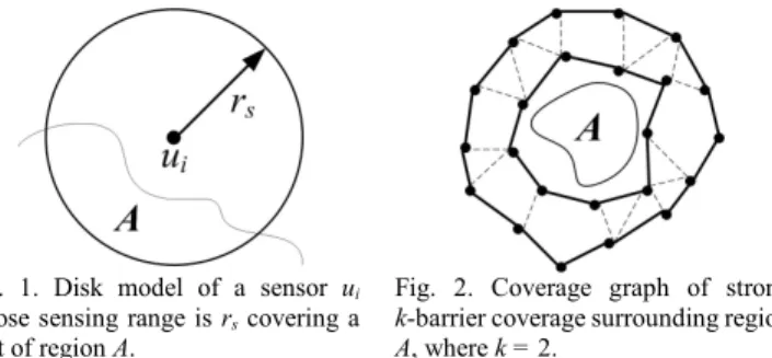
Fig. 1. Disk model of a sensor ui
whose sensing range is rs covering a part of region A.
Fig. 2. Coverage graph of strong k-barrier coverage surrounding region A, where k = 2.
II. BARRIER COVERAGE FORMATION ANALYSIS A. Model
The region of interest A is an area enclosing some types of substance on a 2D plane. Assume that the region is static and has a continuous boundary.
A mobile sensor ui moves with a velocity v on the plane. The sensing area is assumed to be the widely adopted disk model. In this disk with a radius rs, a sensor has the ability to distinguish out whatever substance it is trying to besiege as shown in Fig. 1.
A sensor knows its location information (xi, yi) with equipping affiliated devices such as GPS. The communication range be- tween sensors is rc, where assume rc > 2rs. Generally, the number of sensors n is given before deployment.
Barrier coverage in [2] is described by a coverage graph G(n)
= (V, E). The set V consists of a vertex corresponding to each sensor. An edge exists between two vertexes if their distance is less than 2rs. Strong barrier coverage [5] is presented as a closed chain, which is composed of the edges enclosing the region. Since the sensors have the capability of movement, only strong barrier coverage formation is considered in this study.
The strong k-barrier coverage is referred that there are number k of vertex disjointed chains in G(n). Fig. 2 introduces a k = 2 strong barrier coverage graph. The detection capability is usually measured by the number k.
B. Fundamental Problem Statement
One advantage of barrier coverage is that it saves huge number of sensors than full coverage when protecting a region from intruders. Most studies [2][3][4][5][6] assume that sen- sors without movement ability are randomly deployed around the region. There are also many redundant sensors wasted during the barrier coverage formation. If fewer sensors can form the same strong k-barrier coverage, it will be more bene- ficial in cost.
Obviously, manual deployment can take full advantage of n sensors to set approximate optimal barrier coverage. However, since the region of interest is usually large in scale and the arbitrary deployment task may be dangerous, it is difficult to deploy sensors manually. Therefore, the mobile sensor is con- sidered as one of the best candidates to solve this problem.
The automatic barrier coverage formation problem is defined to be the problem that mobile sensors automatically move from their source positions to form the strong k-barrier coverage for the region of interest.
The objective of solving the problem is to maximize k with given n. Then, all sensors form the maximal k-barriers without
incurring waste. That is to say, given the demand of barrier coverage, the number of sensors will be minimized.
The main difficulty to solve this problem lies in that sensors have only local information by communication and sensing.
Then, how the sensors know their destination and what paths they move along without global information? The destination is analyzed in Subsection C, additional requirements are consi- dered in Subsection D and the path is designed in Section III.
C. Optimal Distribution Pattern
The optimal destination of n vertexes is defined to follow the distribution of consisting maximum k vertex disjointed chains in coverage graph G(n).
Additionally, fc(A) is a function of the length of the convex hull of the region A. The method of obtaining fc(A) can be found in [7]. Thus, we have:
Theorem 2.1 A sufficient condition of achieving maximum k is that n sensors are uniformly distributed on the convex hull of the region A. The maximum value of k is
2 .
( )
s c
k nr
= f A (1)
Proof: We prove this theorem by introducing the following three lemmas.
Lemma 2.1 The shortest perimeter enclosing the region A is its convex hull.
According to convex analysis [7], the smallest area and the shortest perimeter polygon containing a 2D region is its convex hull. Hence, the shortest perimeter equals to fc (A). In other words, the least length of one barrier chain is fc (A).
Lemma 2.2 The longest length consisted by vertexes is 2nrs. Due to the edge definition in coverage graph that an edge exists when d(ui, uj) ≤ 2rs, the longest distance between any two connectable vertexes is 2rs. Connecting n vertexes in series, then, the longest length of all these vertexes is 2nrs.
Wind the series of vertexes to the convex hull of region A.
Combining with Lemma 2.1 and 2.2, the theoretical maximum value of the number of chains k can be computed as
2 .
( )
s c
k nr
= f A
Lemma 2.3 It is a sufficient condition for achieving optimal k that n vertexes are uniformly distributed on the shortest bar- rier perimeter of the region A.
If all vertexes are distributed on the shortest perimeter, sev- eral vertex disjointed chains will overlap completely. In this case, any point on the perimeter is covered by a few sensors.
The least covered number is treated to the k. It can be described that when an intruder crosses the barrier from any path, there are at least k sensors detecting it. This concept is transformed from the strong k-barrier coverage definition in [2] for this case.
In Lemma 2.3, n vertexes are uniformly distributed. Hence, k is equivalent for every point on the perimeter. We have the distance between any pair of adjacent neighbors
( ). f Ac
Δ = n (2)
And any point on the perimeter is covered by at least
2rs . k =
Δ (3)
Combining Eqn. 2 and Eqn. 3, we have
2 2
( ).
s s
c
r nr
k= = f A
Δ (4)
It is the same result as Eqn. 1, which proves the condition is sufficient. Then the result of Theorem 2.1 follows.
D. Alternative Objectives
Generally, the basic objective of max(k) satisfies most prac- tical scenario. However, there are still several alternative ob- jectives remained in barrier coverage formation problem.
First, consider another type of region: dynamic. A dynamic region has a time-varying boundary. Thus, the area or the shape of the region changes over time. An oil leak is such an instance.
Second, consider a more practical distribution of sensors’
source positions: group release. To put all sensors manually at one or just a few points on the boundary of the region corres- ponds to reality. For example, put all mobile sensors in front of the gate of a nuclear factory. And then, the sensors automati- cally move to form barrier coverage surrounding the factory.
These alternative objectives can appear either in single form or in any combination form in barrier coverage formation.
III. ALGORITHM A. Chain Reaction Algorithm
The source position of sensor is assumed to follow random distribution in the basic problem, while the optimal distribution of destination is derived. Then in this section we develop a cooperative algorithm for the sensors moving automatically from their source to destination with only local information.
To solve this problem, we propose a chain reaction algorithm with two steps: boundary seeking and barrier forming.
Step 1: Boundary seeking. Since sensors are randomly distributed on the plane and have only local information, some of them do not know the location of region A. In order to form the barrier, sensors should know the boundary of region. All source positions can be classified into the following three cases.
Case 1: outside the boundary. A sensor ui is defined to be outside the boundary when d(ui, A) > rs. The sensing area of ui
has no overlap with the region A. In this case, in order to find the boundary, a sensor can move along a spiral as shown in Fig.
3(a). This spiral path is applied to boundary detection in [8].
The advantage of this path is that it seeks the boundary with equal probability on all directions and will not miss the region.
Case 2: on the boundary. B(A) is denoted as a function to get the boundary of region A. A sensor ui is defined to be on the boundary when d(ui, B(A)) ≤ rs. The sensing area of ui has partial overlap with the region. In this case, a sensor can select the shortest path to the boundary as shown in Fig. 3(b).
Case 3: inside the boundary. A sensor ui is defined to be in- side the boundary when d(ui, B(A))> rs and the sensing area of sensor ui is included by region A. A sensor in this case can move in a straight line after randomly selecting a direction to the boundary as shown in Fig. 3(c).
(a) (b) (c) Fig. 3(a). A sensor is outside the region. It moves to the boundary spirally.
Fig. 3(b). A sensor is on the boundary. It moves to the boundary directly.
Fig. 3(c). A sensor is inside the region. It moves to the boundary straightly.
Step 2: Barrier forming. After finding the boundary, sen- sors cooperatively move to form the max(k) barrier coverage. A sensor has two directions along the boundary: clockwise and counterclockwise. The nearest neighbor of either direction is denoted as an immediate neighbor. The cooperation is worked through location information transmission among immediate neighbors, which is easy to realize with high energy efficiency and shorter delay. Since each sensor seeks the boundary itself, its neighbor situation is uncertain. There are also three cases of immediate neighbors on the boundary.
Case 1: two immediate neighbors. When a sensor ui has two immediate neighbors ui-1 and ui+1 on each side, virtual force [9]
is produced from these two neighbors. The magnitude of force depends on the distance d(ui, ui-1) and d(ui, ui+1). In order to balance the two forces, a sensor move along the boundary to the position where d(ui, ui-1) = d(ui, ui+1). Moreover, a sensor with its two immediate neighbors can form two angles. The internal angle is defined as the angle facing the region. A sensor should keep the internal angle no more than 180º. In Fig. 4(a), the internal angle of ui is sharp. In order to balance the force, the destination is ui’. In Fig. 4(b), the part of the boundary is con- cave, so the internal angle of ui is more than 180º. In order to balance and keep the angle limitation, the destination is the middle position between ui-1 and ui+1.
Case 2: one immediate neighbor. When a sensor ui has only one immediate neighbor ui+1 on one side, virtual force is pro- duced and the magnitude is denoted as d(ui, ui+1). Due to this force, sensor ui walks towards the direction without the imme- diate neighbor until d(ui, ui+1) = 2rs.
Case 3: no neighbor. When a sensor has no neighbor in its communication range, there is no virtual force for it to move.
Due to the virtual force in these three cases, sensors can move cooperatively. All sensors move until they are uniformly distributed on the convex hull of the region while all virtual force is balanced. Obviously, the barrier forming is a chain reaction process. Hence, it needs time to converge to steady
(a) (b) (c) Fig. 4(a). Sensor ui has two immediate neighbors and its internal angle < 180o. It
moves to a position on the boundary where d(ui, ui-1) and d(ui, ui+1).
Fig. 4(b). Sensor ui has two immediate neighbors and its internal angle ≥ 180o. It moves to a position that is the middle of ui-1 and ui+1.
Fig. 4(c). Sensor ui has only one immediate neighbor. It moves away from its neighbor ui-1 at 2rs distance and along the boundary of region A.
state.
The metrics to measure the quality of automatic barrier formation algorithm include the travel distance of sensors and the time of formation duration.
The detailed algorithm is shown as follows:
Chain Reaction Algorithm (Executed on sensor ui) Input: the sensing range rs,
while True do
Sense the substance of region A with in rs disk;
switch (Location)
case outside boundary: spiral_moving(); break;
case on boundary: direct_moving(); break;
case inside boundary: straight_moving(); break;
// step 1 finish
Get current location information pc;
Detect the immediate neighbors ui+1 and ui-1; Exchange position information with ui+1 and ui-1; //p is the next position ui will to move, θ is the internal angle
switch(Num of immediate neighbors) case 2:
if(θ ≥ 180) p ← middle point of ui+1 and ui-1;
else p ←q where d(pui+1 ,q) = d(pui-1 ,q) and d(q, A) = 0;
break;
case 1: p ← q where d(pui±1 ,q) = 2rs and d(q, A) = 0;
break;
default: p ← pc; break;
Move to p along the boundary of the region;
// step 2 finish end while
B. Algorithm Extension
For the dynamic region, most parts of chain reaction algo- rithm can be hold. Only one function demands to be comple- ment, which a sensor should keep seeking the time-varying boundary instead of relocating once. The boundary seeking step is executing continuously while forming the convex hull with other sensors. This algorithm can also be used in the barrier reformation situation when some sensors are failure.
For different distribution of sensors’ source positions, no matter following the Gauss, Poisson or any other distribution, the chain reaction algorithm is available without any modifi- cation. For instance, in the group release case, the source posi- tion can be treated that all sensors are deployed at the same location, which is only a special case for distribution. Hence, the basic algorithm is sufficient.
IV. PERFORMANCE EVALUATION A. Simulation Settings
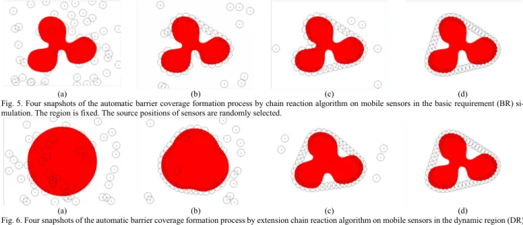
In the basic requirement (BR) simulation, the region of in- terest is set red as Fig. 5(a) and the other part of the plane is set white. The red region has a continuous boundary and its shape is fixed. The size of the plane is set to be 800*600m. There are 50 mobile sensors deployed on this plane, whose source posi- tions are randomly selected. We assume that a sensor can detect and distinguish red or white within its sensing range rs = 25m.
Sensors can transmit information in their communication ranges rc = 60m. The velocity of a sensor is at most 10m/s.
In the dynamic region (DR) case, the red region transforms from a circle to the shape as shown in Fig. 6(d) in 500s.
In the group release (GR) scenario, 50 sensors are set in the same location (301, 109) for their source positions as fig. 7(a).
We implement the chain reaction algorithm and extension algorithms in these simulation cases. Fig. 5, 6 and 7 show the different instants obtained by the algorithms.
B. Performance Analysis
The results of Fig. 5, 6 and 7 verify the validity and gene- rality of our algorithms in solving automatic barrier coverage formation problem. Finally, they all form barrier coverage with k = 2.
In Fig. 8, the accumulated travel distance over time is shown.
As we know, a short travel distance can be treated as lower energy consumption on movement. The total travel distance in three cases is 61367m, 48089m and 43743m at 500s respec- tively. Since sensors have no global information, the redundant travel distance is inevitable such as zigzag path in seeking boundary. However, in the simulation, we find that there is little turning back for sensors with our algorithms, which means only little energy wasted on movement. Among the three curves in Fig. 8, we find that BR has the most accumulated travel dis- tance over time compared to DR and GR. The reason is that the zigzag seeking path costs much travel distance. In DR, the initial region is so large that there are fewer sensors outside the region than those in BR. And the sensors in GR do not require the boundary seeking step.
Moreover, we study the convergence duration. The conver- gence condition for a sensor is that the distance between its current position and next position is less than a threshold of 0.1m. When all sensors achieve the convergence condition, the barrier coverage formation process is completed. With this condition, all the three simulations can converge. From Fig. 9, we obtain the durations are 855s, 685s and 510s, respectively.
We find that BR is the slowest process to converge compared to DR and GR. The reason is that the sensors in BR cost the most time to seek the boundary while the least in DR.
V. CONCLUSION
The problem of automatic barrier coverage formation by mobile sensors is addressed in this paper. The chain reaction algorithm is proposed on sensors to move automatically and cooperatively from their source positions to form maximal k strong barrier coverage. This algorithm can be widely applied to different initial states such as random or arbitrary deploy- ment. It could also be extended to protect the dynamic region.
Since the barrier coverage formation problem is newly raised, there exist several open questions for further study. One of our future works is that the movement ability of mobile sensors is constrained by the terrain situation. For example, the obstacles exist on the plane. Second, energy problem is critical for mobile sensors. To study the optimal path of minimal travel distance for all sensors is another future work.
VI. ACKNOWLEDGEMENT
This research was partially supported by NSF of China under grant No. 60773091, 973 Program of China under grant No.
2006CB303000, Key Program of National MIIT under Grants no. 2009ZX03006-001 and 2009ZX03006-004.
REFERENCES
[1] I. Akyildiz, W. Su, Y. Sankarasubramaniam, and E. Cayirci. “Wireless Sensor Networks: A Survey”, Computer Networks Journal, 38(4): pp.
393–422, 2002.
[2] S. Kumar, T. H. Lai and A. Arora, “Barrier Coverage with Wireless Sensors”, ACM MobiCom, Germany, 2005.
[3] A. Chen, S. Kumar, and T. H. Lai. “Designing Localized Algorithms for Barrier Coverage”, ACM MobiCom, Canada, 2007.
[4] P. Balister, B. Bollobas, A. Sarkar, and S. Kumar, “Reliable Density Estimates for Coverage and Connectivity in Thin Strips of Finite Length”, ACM MobiCom, Canada, 2007.
[5] B. Liu, O. Dousse, J. Wang, and A. Saipulla, “Strong Barrier Coverage of Wireless Sensor Networks,” ACM MobiHoc, 2008.
[6] A. Saipulla, C. Westphal, B. Liu and J. Wang, “Barrier Coverage of Line-Based Deployed Wireless Sensor Networks”, IEEE INFOCOM, Brazil, 2009.
[7] RT. Rockafellar, “Convex Analysis”, Princeton University Press, 1997.
[8] J. Clark and R. Fierro, “Cooperative Hybrid Control of Robotic Sensors for Perimeter Detection and Tracking”, American Control Conference, Portland, OR, USA, 2005.
[9] Y. Zou and K. Chakrabarty, “Sensor Deployment and Target Localization Based on Virtual Forces”, IEEE INFOCOM, USA, 2003.
(a) (b) (c) (d) Fig. 5. Four snapshots of the automatic barrier coverage formation process by chain reaction algorithm on mobile sensors in the basic requirement (BR) si-
mulation. The region is fixed. The source positions of sensors are randomly selected.
(a) (b) (c) (d) Fig. 6. Four snapshots of the automatic barrier coverage formation process by extension chain reaction algorithm on mobile sensors in the dynamic region (DR)
simulation. The region is time-varying. The source positions of sensors are randomly selected.
(a) (b) (c) (d) Fig. 7. Four snapshots of the automatic barrier coverage formation process by chain reaction algorithm on mobile sensors in the group release (GR) simulation.
The region is fixed. All sensors are released in the same position at the beginning.
Fig. 8. The accumulated travelled distance of all sensors over time. Fig. 9. The convergence duration of chain reaction algorithm.