Joint Optimization of Multicast Energy in Delay-constrained Mobile Wireless Networks

(1)

Joint Optimization of Multicast Energy in Delay-constrained Mobile Wireless Networks

Luoyi Fu¹, Xinzhe Fu¹, Zesen Zhang², Zhiying Xu², Xudong Wu¹, Xinbing Wang^1,2, and Songwu Lu³

1Dept. of Computer Science, Shanghai Jiao Tong University, China.

Email:{yiluofu,fxz0114,xudongwu,xwang8}@sjtu.edu.cn.

2Dept. of Electrical Engineering, Shanghai Jiao Tong University, China.

Email:{zesenzhang,xuzhiying}@sjtu.edu.cn

3Dept. of Computer Science, University of California, Los Angeles, USA. Email:{slu}@cs.ucla.edu

Abstract—This paper studies the problem of optimizing multicast energy consumption in delay-constrained mobile wireless networks, where information from the source needs to be delivered to all the k destinations within an imposed delay constraint.

Most existing works simply focus on deriving transmission schemes with the minimum transmitting energy, overlooking the energy consumption at the receiver side. Therefore, in this paper, we propose ConMap, a novel and general framework for efficient transmission scheme design that jointly optimizes both the transmitting and receiving energy. In doing so, we formulate our problem of designing minimum energy transmission scheme, called DeMEM, as a combinatorial optimization one, and prove that the approximation ratio of any polynomial time algorithm for DeMEM cannot be better than ¹₄ln k. Aiming to provide more efficient approximation schemes, the proposed ConMap first converts DeMEM into an equivalent directed Steiner tree problem through creating auxiliary graph gadgets to capture energy consumption, then maps the computed tree back into a transmission scheme. The advantages of ConMap are threefold- ed: i) Generality– ConMap exhibits strong applicability to a wide range of energy models; ii) Flexibility– Any algorithm designed for the problem of directed Steiner tree can be embedded into our ConMap framework to achieve different performance guarantees and complexities; iii) Efficiency– ConMap preserves the approximation ratio of the embedded Steiner tree algorithm, to which only slight overhead will be incurred. The three features are then empirically validated, with ConMap also yielding near- optimal transmission schemes compared to a brute-force exact algorithm. To our best knowledge, this is the first work that jointly considers both the transmitting and receiving energy in the design of multicast transmission schemes in mobile wireless networks.

Index Terms—Mobile Wireless Networks, Energy Optimiza- tion, Multicast

I. INTRODUCTION

With the surge of mobile data traffic, energy consumption in communication is rising radically in recent years. As reported by a survey [1] where Telecom Italia is said to be the second largest consumer in Italy, energy consumption of mobile communication is already ranking the top. Hence, energy saving becomes a crucial issue that receives considerable attention in the design and implementation of mobile wireless networks.

The early version of this paper is to appear in the Proceedings of ACM MobiHoc 2017 [40].

As the majority of nodes are battery powered, a key problem of energy cost reduction in mobile wireless networks is to find a route with minimum total energy consumption for a given communication session [2]. Under such circumstance, multicast turns out to be more efficient due to the increasing demand of information sharing in those communication scenarios.

It outperforms unicast by aggregating multiple flows from the same source so that network resources such as capacity and energy can be saved. However, as a traffic pattern that generalizes both unicast and broadcast, the issue of minimum- energy multicast is far more complicated compared to that of minimum-energy unicast, which is essentially a shortest path problem in static network.

Among existing works that indeed study the minimum- energy multicast problem, most of them [3], [4] are limited to static networks, which fail to well characterize many realistic scenarios where users are manifested to be moving. Conse- quently, the potential energy saving brought with mobility is also overlooked. Another concern lies in that the state of art mostly focuses on optimizing the energy consumed only at the transmitting side [5], [6], but does not take into consideration the receiving energy, which, as suggested by empirical studies [7], [8], is as significant as the transmission cost. Further- more, due to the possible collisions and retransmissions in multicast/broadcast protocols, the energy consumption is not synonymous at transmitting and receiving sides. Interpreted in a more detailed way, the energy consumption of the transmitting side is usually determined by transmitting power, while at the receiving side, taking reliable MAC layer multicast as an example [9], the energy consumption may depend on the number of intended recipients as each transmission involves waiting for feedback from the receivers and resending the missing packets. Such inherent heterogeneity between transmitting and receiving energy can also be found in many other real applications such as wireless multihop networks [10] and full-duplex energy harvesting infrastructures [11]. Therefore, it is difficult to directly embed the receiving energy into existing algorithms. These motivate us to propose a general framework that jointly optimizes both the transmitting and receiving energy in mobile wireless networks.

In addition to the energy, our framework needs to incorporate the latency, another crucial performance metric, of

(2)

which the demand varies in different scenarios. Real time applications such as video conferencing and traffic monitoring require the network latency to be fairly small, whereas in other networks (e.g. satellites network), network delay is not so critical. Hence, it is reasonable to add to the network a delay constraint, meaning that all the packages must be delivered within a time length of D. Based on that, all the above cases can be well characterized by simply adjusting the size of D. Following this, there emerge a flurry of studies that quest for the relationship between delay constraint and other network performances. For instance, Small et al. show that relaxing delay constraint can bring about energy reduction or throughput gain [12]. Ra et al. propose an online algorithm for achieving near optimal energy-delay tradeoff in smartphone applications [13]. However, current literature on energy-delay tradeoff is limited to some specific applications, where the main goal is to empirically optimize the tradeoff without the corresponding theoretical exploration [13], [14]. Under such circumstance, two questions still remain open:

• How hard is it to achieve the minimum multicast energy under delay constraint in mobile wireless networks?

• How should we efficiently design such optimal multicast transmission schemes with minimum energy consumption in delay-constrained mobile wireless networks?

We therefore present a first look into the problem of multicast energy consumption optimization in delay-constrained wireless mobile networks, with both transmitting and receiving energy considered. Specifically, we consider a multicast session with k destinations selected in advance from all the n nodes in the network. With time divided into equal slots, we impose a delay constraint D on the multicast session in the sense that packets from the source must be delivered to all the k destinations within D time slots. We aim to design efficient multicast routing schemes that achieve the minimum transmitting and receiving energy. Unlike traditional multicast in wired network, which is essentially a minimum Steiner tree problem, the issue becomes more complicated when it comes to mobile wireless mulitcast. First, network topology is time-varying due to the mobility of nodes. This makes the task of designing an optimal transmission scheme rather challenging since the same tree may correspond to many different transmission schemes. Second, the “broadcast nature”

in wireless communication, to a large extent, complicates the calculation of energy consumption since it cannot be obtained by simply taking the summation of edge weights in a minimum Steiner tree problem.

We approach the problem of multicast energy optimization in delay-constrained wireless mobile networks by formulating it as a combinatorial optimization problem called the DeMEM problem. Upon theoretical analysis on the approximation hardness of the DeMEM problem, we propose a novel energy optimizing framework called ConMap. Particularly, ConMap realizes multicast transmission in three major steps. First, it constructs an intermediate graph resulted from snapshots of graph states taken under D different slots and auxiliary gadgets for transmitting and receiving energy; Second, it builds a Steiner tree in that intermediate graph spanning all the

destinations; Finally, it maps the obtained tree in that intermediate graph back into a multicast transmission scheme in the original network. The proposed ConMap flexibly allows us to embed any directed Steiner tree algorithm into it, and turns out to be efficiently implementable with only a polynomial time complexity as well as preserving the approximation ratio of the underlying directed Steiner tree algorithms. Our main contributions are listed as follows:

• We prove that the approximation ratio of DeMEM problem in mobile wireless networks cannot be better than ¹₄ln k for any polynomial-time algorithm, which is an even stronger result than demonstration of its NP- hardness.

• We propose ConMap, a novel framework that jointly optimizes the transmitting and receiving energy in the multicast session and harnesses the results of existing directed Steiner tree algorithms to achieve a good approximation for DeMEM. Our framework does not rely on any specific characterization of energy consumption and is thus applicable to a broad range of applications.

• We empirically evaluate the performance of ConMap on real datasets, where ConMap exhibits good applicability to real network traces and yields near optimal transmission schemes compared to a brute-force exact algorithm. We also demonstrate the significance of jointly optimizing transmitting and receiving cost by showing that incorporating receiving energy into ConMap leads to transmission schemes of lower energy consumption.

The rest of this paper is organized as follows: Section II is contributed to literature review and we introduce our network and energy models in Section III. We prove the approximation hardness of DeMEM in Section IV. The approximation framework, ConMap, is proposed in Sections V and VI. We conduct simulations to evaluate the performance of our framework in Section VII and give concluding remarks as well as future directions in in Section VIII.

II. RELATEDWORK

A. Minimum Energy Multicast-related Problems

In the literature, the problem of transmitting energy consumption optimization is referred to as Minimum-Energy Multicast (MEM) problem, and has been extensively studied in static networks. Since both MEM problem and Minimum- Energy Broadcast (MEB) problem, a special case of MEM, are proven to be NP-hard [15], [16], [17], the community focuses on designing efficient heuristics. Wieselthier et al.

study the MEM problem using the same approach as the MEB problem and propose three greedy heuristics [16], [3].

Wan et al. prove that both MEM problem and MEB problem can be approximated within constant ratio [4], [18]. Liang et al. propose approximation algorithms for MEB problem where the nodes have discrete transmission power levels [17].

Existing works also relate to the extensions of MEM and MEB such as MEM and MEB problem with reception cost [19], [9], duty-cycle-aware MEM [6] and delay-constrained MEM [5]. Furthermore, energy efficient multicast/broadcast algorithms for specific applications is also an active topic

(3)

[20]. Gong et al. propose an efficient distributed algorithm for multicast tree construction in wireless Sensor Network [21]. However, as noted earlier, prior literature only focuses on the minimization of transmitting energy, relies on the assumption that the receiving energy is directly proportional to the number of receivers [19] or considers the receiving energy in the context of network-wide broadcast [9]. In contrast, the proposed framework in our work jointly minimizes the transmitting and receiving energy, with applicability to more general scenarios.

In spite of a flurry of works addressing the issue of MEM in static networks, little is known about the energy consumption in mobile scenarios. As two exceptions, Wu et al. [22] study MEM in mobile ad hoc networks using network coding, but their focus is on energy gain from network coding rather than mobility. Guo et al. [2] propose an efficient Distributed Min- imum Energy Multicast algorithm, but how delay constraint affects the energy consumption is not considered. In many cases where the timely delivery of messages is not of primary concern, relaxing delay constraint can bring gain in many aspects such as capacity and energy [12]. Considerable efforts have been made to investigate the theoretical delay-capacity relationship in large scale static and mobile wireless networks [23], [24], [25], [26].

Despite those dedications to multicast energy optimization, as far as we know, there is no prior work, other than ours, that considers the problem of jointly optimizing transmitting and receiving energy of multicast in mobile wireless networks.

B. Stochastic Network Control

Apart from the aforementioned works that mostly rely on graphical modeling of networks and deterministic packet arrival that are analogous to ours, there are a different line of research in the area of stochastic network control that deals with similar issues of network performance optimizations. The pioneering work of Tassiulas and Ephremides [27] studies the throughput optimal (unicast) routing policy of parallel-queue networks. The policy they proposed are subsequently referred to as back-pressure routing, and the Lyapunov-drift argument they applied set the basis for many works that follow. Neely et al. extend the throughput-optimal back pressure routing to time varying wireless networks [28]. Neely also proposes an energy-optimal unicast routing algorithm for time varying wireless networks [29]. Generalizing the unicast transmission pattern, Sinha et al. propose throughput optimal routing policy for multicast, broadcast and anycast transmission in wireless networks [30], [31]. Interested readers can refer to [32] for a complete survey and tutorial on this topic.

It is meaningful to distinguish our work from the aforementioned research in stochastic network control and analyze their pros and cons. Although the two kinds of works both focus on designing transmission/routing schemes with desirable properties, the feasibility of the schemes are defined in different fashions. In our work, a transmission scheme is feasible if all the designated destinations can successfully receive the packets within the delay constraint (as will be formally defined in Section III). While, in stochastic network control, each

network node is associated with a queue for packets, and the feasibility condition of the transmitting policies are that the long term time average queue backlogs for all nodes must be finite. The routing schemes designed in latter kind of works [27], [28], [29] make transmitting decisions in a distributed manner only based on nodes’ queue backlogs. This gives them an advantage as the policies can achieve the properties without the knowledge of future packets arrival, future nodes mobility, etc [30], [31]. However, as the feasibility condition is defined using the time average instead of deterministic short term conditions, the algorithms in the latter works cannot be applied to derive delay-constrained transmission schemes. Indeed, the class of back pressure policies [32] often incur high packet delay that increases with the size of the networks. On the other hand, the algorithm designed in our work yields transmission schemes with constant delay (under a certain delay constraint threshold) and is approximately energy optimal.

III. MODELS ANDASSUMPTIONS

A. Mobile Wireless Network Model

We adopt the mobile wireless network model in [33] that can be reproduced as follows: time is divided into discrete time slots and the nodes remain static within a time slot. And this model permits a reasonable prediction of nodes’ future movements. The reason behind is that the node mobility and the evolution of topology are heavily dependent on social and temporal characteristics of the network participants. And there are lots of examples such as the easy discovery of the topology for a DTN formed by public buses [41]. And more details of reason can be referred to [33]. With reasonable prediction of nodes’ future movements, a mobile network can be modeled as a sequence of static graphs G = {G1, G₂, . . .}, with each static graph interpreted as a snapshot of nodes’ positions in a time slot. Specifically, denoted as G_t(V, E_t, w_t) ∈ G, each static graph is a weighted directed graph with V = {v₁, v₂, . . . , v_n} corresponding to the n network nodes. Et⊆ V ×V denotes the edge set and wt: Et7→ R⁺assigns each edge a corresponding weight. An edge e = (vi, vj) ∈ Et means that vi can send messages to vj in time slot t with minimum transmission power wt(e).

B. Multicast Model

We consider a wireless multicast session with a source s ∈ V and destination nodes set T ⊆ V in mobile network G.

We impose an integral delay constraint D on the multicast session in the sense that the message must be delivered to all nodes in T within D slots. Therefore, for a mulicast session, we only need to consider the network snapshots within the delay constraint. Hence, in the sequel, we truncate the mobile network G into D static graphs denoted as {G1, G2, . . . , GD}.

Since we aim to design a minimum energy transmission scheme for a delay-constrained multicast session in a mobile wireless network, we next formally define the notion of transmission scheme. We refer to the process of some transmitter transmitting message to the intended receivers as a transmission. A transmission scheme specifies the transmitter, intended receivers, timing and transmission power of each transmission.

(4)

time

space

1

t = t =2 t =3 t =4 time

space

source

destination reached nodeunreached node intended receiver

v1 v¹

v2

v3

v4

v5 v⁵ v₅ v5

v6

1

t = t =2 t =3 t =4

v1 v¹

v2

v3

v4

v5 v⁵ v₅ v5

v6

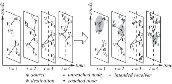
Fig. 1. A mobile wireless network and a feasible transmission scheme for a multicast session in the network; (a) a mobile wireless network (a sequence of snapshots); (b) a feasible transmission scheme for a multicast session in the network with v1 being the source, v4, v6 being the destinations and a delay constraint of four time slots.

Definition 1: A transmission scheme π ⊆ V × 2^V × {1, . . . , D}×R⁺is a sequence of tuples {(u, V⁰, t, p)}, where a tuple τ = (uτ, Vτ, tτ, pτ) ∈ π denotes that node uτ should transmit to the nodes in Vτ at time slot tτ with power pτ. Also, in a transmission scheme π, we define a node to be

“reached in time slot t” in a recursive way as follows: (i) the source s is reached in time slot 1, (ii) if a node is reached in time slot t, then it is reached in time slot t⁰ for all t⁰ ≥ t, and (iii) if a node u is reached in time slot t and (u, V , t, p) ∈ π), then all nodes in V are reached after time slot t, or we say they have been reached in time slot t + 1. Now, we give the definition of feasible transmission scheme and will restrict our consideration to the set of feasible transmission schemes in the sequel. Intuitively, a scheme is said to be feasible if it is without redundancy and qualified for the delay constrained multicast session.

Definition 2: A transmission scheme π is feasible if it ob- serves the following conditions: (i) For all τ = (u, V⁰, t, p) ∈ π, it satisfies that u is reached in t and for all v ∈ V⁰, e = (u, v) ∈ E_t and p ≥ maxe=(u,v)∈E_t,v∈V⁰{wt(e)}. (ii) For all τ = (u, V⁰, t, p) ∈ π, no node in V⁰ is reached before t. (iii) All nodes in T are reached in time slot D.

Figure 1 illustrates an example of a mobile wireless network, along with a feasible transmission scheme proposed under a multicast session in the network.

The transmission scheme corresponding to the tuples {(v₁, {v₂, v₄}, 1, p₁), (v₂, {v₅}, 2, p₂), (v₅, {v₆}, 4, p₃)}.

C. Energy Model

For a transmission specified by tuple τ = (uτ, Vτ, tτ, pτ), we model the energy consumption of this transmission as

E(τ ) = pτ+ f (|Vτ|),

where the first part denotes the energy consumed by the transmitter side and f is a function of the number of intended receivers that can represent the receiving energy. Note that our framework does not restrict to any specific f and the choice of f may depend on practical settings [7], [9], which will be specified in Section VI. It follows that the energy consumption of a transmission scheme π is given by:

E(π) =X

τ ∈π

E(τ ).

Now we formulate the DeMEM problem as follows.

Definition 3: (The DeMEM Problem) Given a mobile wire- less network G = {G1, G2, . . . , GD}, a source node s, a set T of destination nodes, and a delay constraint D, the goal is to find a feasible transmission scheme with minimum energy consumption.

We note that in the definitions above, we make the following characterizations of communication in mobile wireless networks. First, we assume that the transmission rate is much faster than that of the nodes’ mobility. In other words, it is feasible to transmit multiple times to different receivers in a single time slot. This may not be desirable if we only consider transmission cost. However, it can bring possible gain when we take the receiving energy into account. Second, we can utilize the wireless broadcast nature during communications, i.e., different nodes can be reached within one transmission as long as the transmission power is large enough. Third, in the present work, we focus on the multicast of one data packet in the network, which alleviates us from the burden of interference and packet scheduling issues. We leave the minimum energy multicast with a streaming of packets as future work.

IV. APPROXIMATIONHARDNESS

In this section we analyze the approximation hardness of DeMEM problem. We show that even without receiving energy (i.e., f = 0), the DeMEM problem cannot be approximated within a /textcolorredlogarithmic factor in polynomial time by reduction from acyclic directed Steiner tree problem.

Theorem 1: The DeMEM problem cannot be approximated in polynomial time within a factor better than ¹₄lnk, where k is the number of destination.

Proof: Consider an instance of acyclic directed Steiner tree problem defined by an acyclic directed graph G(V, E) and an edge cost function d : E → R⁺, a root r ∈ V and a set of vertices S ⊆ V with |S| = k. The goal is to find a minimum cost Steiner tree (arborescence) covering all vertices in S. Based on these, we will construct an instance of the DeMEM problem by encoding the graph information into a mobile wireless network.

To begin with, we do a topological sort on the graph and get a sequence of nodes following the topological order. Without loss of generality, we only consider the nodes that do not lie before the root r in the sequence, i.e., a truncated sequence {r = v0, v1, . . .}. Then, we sort the relevant edges according to the order of their outgoing nodes in the truncated sequence into {e0, e₁, . . . , e_l}. From this sequence, we will build a mobile wireless network G.

First, we set V⁰ as the set of nodes that appear in the truncated sequence. Then, for any generic edge ei= (ui, vi) in the edge sequence, we add (ui, vi) into Gi(V⁰, Ei, wi) and set its cost as wi(e) = d(e). The constructed network G consists of static graphs {G1, G2, . . . , Gl} where each static graph has only one edge. Further, we designate r as the source, the nodes corresponding to the vertices in S as the destinations, and set the delay constraint D = l, the receiving energy function as zero. By above procedures, we have an instance of DeMEM

(5)

problem and now we show that it is equivalent to the original acyclic directed Steiner tree instance.

For a Steiner tree in G, if it contains edges {e_y₁, e_y₂, . . . , e_y_j}, then obviously the corresponding transmission scheme with tuples {(uy₁, {vy₁}, y1, d(ey₁)), . . . , (uy_j, {vy_j}, yj, d(ey_j))} is feasible. Conversely, consider a feasible transmission scheme for the mobile wireless network. Since in each time slot there only exists one edge, each tuple in a feasible transmission scheme corresponds to some edge in the acyclic graph G. And from the requirements for the scheme to be feasible, it follows that those edges form a Steiner tree in G. Most importantly, the energy consumption of a feasible transmission scheme equals to the cost of its corresponding Steiner tree and all the reduction processes are implementable in polynomial time. Therefore, the above reduction is an approximation preserving reduction. Since for a fixed k there is no efficient

1

4ln k approximation for acyclic directed Steiner tree problem unless NP⊆ DTIME(n^polylogn) [34], we obtain the same approximation hardness for DeMEM problem.

V. THEAPPROXIMATIONFRAMEWORK: CONMAP

Since by Theorem 1, even approximating the DeMEM problem better than a logarithmic factor is NP-hard, it is unlikely that the DeMEM problem can be solved in polynomial time.

Therefore, we need to design efficient approximation scheme to trade complexity for the optimality of the transmission scheme. In this section, we therefore propose a novel approximation framework – ConMap, which effectively achieves such tradeoff by transforming our DeMEM problem into a directed Steiner tree problem.

Given a specific DeMEM problem instance, ConMap first converts the mobile wireless network graph to an intermediate graph, then adopts established algorithms to compute an approximate minimum Steiner tree in the intermediate graph, and finally uses the computed Steiner tree to construct a near optimal transmission scheme for the original DeMEM problem. As we will disclose in the sequel, all the conversion processes are efficiently implementable, with a polynomial time complexity and the size of the intermediate graph being polynomial to that of the original network graph. Also, we can embed different algorithms for directed Steiner tree to obtain various performance guarantees.

Here for clarity and convenience, we first consider DeMEM problem without receiving energy and will demonstrate in Section VI how to integrate the receiving energy into the optimization.

A. Conversion into an Intermediate Graph

To derive an energy efficient transmission scheme, we firstly need to generate an intermediate graph so that the mobility of nodes and the broadcast nature of wireless environment can be captured. Note that the intermediate graph is a directed layered graph, with each layer corresponding to the network at a certain time slot.

Given a mobile wireless network G = {G1, G2, . . . , GD}, before we construct an intermediate graph, we adopt previous

assumption [17] that there are pvadjustable transmitting power levels for a generic node v. Note that even for nodes with infinitely adjustable transmitting power, there are at most (|V |−1) power levels that need to be taken into consideration.

Upon the power level assignment, we can now construct an intermediate graph at layer t by applying to all nodes the procedures listed as follows, with the resulting layer denoted as Lt:

1) Create a vertex in Ltfor each node in Gtand call these vertices “original vertices”.

2) For the pu power levels of node u, add a set of vertices denoted as {w_u1, w_u2, . . . , w_up_u} to the graph L_t. Hereby, without ambiguity, we will also refer to these vertices as “power levels” and their labels as their corresponding transmission powers.

3) Add a directed edge from u to each of its power levels and set the edge’s weight as the transmission power consumed by u when transmitting at that power level.

4) Add edges from wuj to all the vertices that can be covered by u when transmitting at power level j and assign their weights as zero. Formally, a vertex v can be covered by u at power level j if and only if

∃e = (u, v) ∈ Et and wt(e) ≤ wuj.

Upon the construction of D layers that correspond to D time slots, we connect them into the intermediate graph. Starting from L1, we establish the relation of adjacent layers by adding zero-weight edges between the original vertices in them that correspond to the same node in different time slots. These edges resemble the temporal links in the model of [33], with their directions following the chronological order. With all the operations above, we complete the construction of the intermediate graph denoted as L, which, in the sequel, will be demonstrated to well capture both node mobility and the broadcast nature of wireless networks.

B. Computation of the Steiner Tree

We designate in L1 the vertex that corresponds to the source node in the network as the root r and in LD the original vertices that correspond to k destinations as terminals.

Therefore, the DeMEM problem is equivalent to establishing a minimum Steiner tree rooted at r spanning all k terminals in the intermediate graph L. Recall that in the intermediate graph, the weight of edges from original vertices to their power levels equals to the transmission power. And the weights of edges from power levels to the original vertices they cover are zero. It follows that the weight assignment ensures that the summation of the weights of edges in a Steiner tree characterizes the energy consumption of a wireless multicast session. In addition, the directed layering structure of the intermediate graph captures the nodes’ mobility and ensures that the Steiner tree in L will be generated following the chronological order. Hence, the intermediate graph L is an accurate abstraction of mobile wireless network.

Since our task now becomes computing the minimum Steiner tree in a directed graph, we can adopt existing efficient approximate algorithms [35], [36] to fulfill our purpose. With considerable efforts of searching an approximate algorithm

(6)

that runs in polynomial time, the best algorithm available is still linear with n but exponential with k, with unsatisfacto- ry approximation ratio. However, for completeness, we still present the result in the following lemma.

Lemma 1: There exists an algorithm that provides an l(l − 1)k¹^l approximation to Steiner tree problem in directed graph in time O(n^lk^l+n²k+nm) where n is the number of vertices, k is the number of terminals and m is the number of edges.

Specifically, set l = log k, we get an 2 log²k approximation in time O((nk)^{log k}) [35], [37].

Through implementation of the Steiner tree algorithm, we obtain an approximate Steiner tree in our intermediate graph, which will serve as the basis for the construction of transmission scheme.

C. Mapping into the Transmission Scheme

Based on the Steiner tree we computed, we proceed to design the corresponding transmission scheme. First, we present a crucial property of the conversion process.

Lemma 2: For an instance M of DeMEM problem, let M⁰ be the directed Steiner tree instance converted from M by ConMap framework. Each feasible transmission scheme in M corresponds to a valid Steiner tree in M⁰, and the energy consumption of the scheme equals to the cost of its corresponding Steiner tree.

Proof: We describe a procedure that maps a feasible transmission scheme π for M to an edges set ET that forms a Steiner tree for M⁰. For each tuple (u, V⁰, t, p) ∈ π, we add the edge from u to the power level corresponding to p in layer L_t together with the edges from the aforementioned power level to the original vertices of vertices in V⁰ of L_t into ET. Finally, we add the necessary inter-layer edges into the set. The edge set constructed by the above procedure will be a valid Steiner tree for M⁰. In the sequel, we refer to the Steiner trees that have corresponding transmission schemes as being in canonical form.

From the proof of Lemma 2, we note that the energy consumption of any scheme is no less than the cost of the optimal Steiner tree in the constructed instance. Therefore, a transmission strategy mapped from an α-optimal Steiner tree is guaranteed to be an α-optimal transmission scheme. However, the Steiner tree computed in the intermediate graph may exhibit “aberrant phenomena” so that it has no corresponding feasible transmission scheme. Hence, in the final phase of ConMap, before we map our computed Steiner tree back into a transmission scheme, we need to prune it into canonical form.

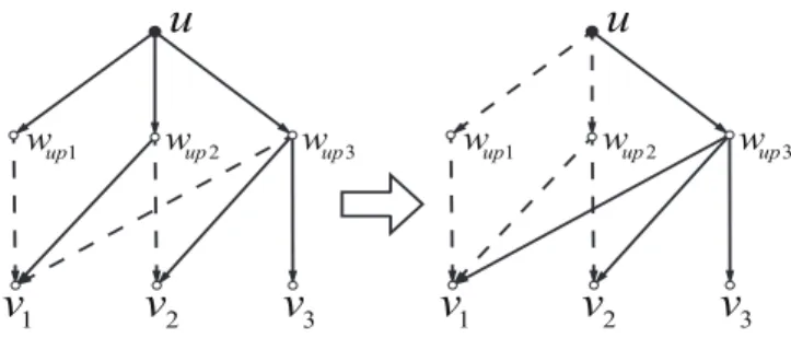
The possible aberrant phenomena that can cause a Steiner tree ET not to have its corresponding feasible transmission scheme is: there are edges from different power levels to multiple original vertices that correspond to the same network node, leading to redundant transmissions. To deal with this case we keep the edge with the original vertex in the earliest time slot and delete other redundant edges. An example of the pruning procedure is illustrated in Figure 2. Then, we add necessary inter-layer edges to reconnect the resulting edge set into a Steiner tree. Note that the above two procedures do not increase the cost of the resulting Steiner tree. Therefore, the pruned Steiner tree can only be closer to optimal.

u

1

wup w_up₂ w_up₃

v

1

v

2

v

3

u

1

wup w_up₂ w_up₃

v

1

v

₂

v

₃

Fig. 2. Illustration of the pruning procedure in ConMap without receiving energy. The left part denotes a subgraph of a constructed Steiner tree that is not in canonical form. The right part represents the corresponding subgraph after the pruning procedure: absorb the original vertices that are connected to wup2 into wup3. And the solid lines are the way that we have chosen to transmit and the dashed lines present the way that we have not chosen.

After describing the three main stages of the framework, we summarize ConMap in Algorithm 1.

Algorithm 1 ConMap Steiner Framework for DeMEM Input: An instance of the DeMEM problem M Output: A transmission scheme π for M

1: Construct the corresponding intermediate graph L of M and form an instance of directed Steiner tree M⁰.

2: Compute a (approximate) minimum Steiner tree ET in L for M⁰.

3: Prune ET into canonical form.

4: Convert the pruned ET to its corresponding transmission scheme π for M.

D. Illustration of ConMap

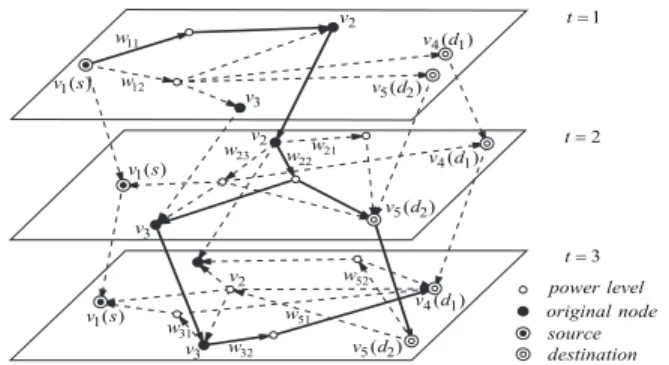
Now we illustrate our proposed framework, ConMap, using an example of a five-node mobile network, where multicast is between one source and two destinations with a delay constraint of three time slots. Figure 3 shows the intermediate graph of the network. Note that we omit some of the power levels due to space limitations. As shown in the figure, v1

corresponds to the source, v4 and v5 correspond to the destinations. The solid lines denote the Steiner tree the algorithm computes in the intermediate graph. Here, the transmission scheme is {(v1, {v2}, 1, w11), (v2, {v3, v5}, 2, w22),

(v3, {v4}, 3, w32)}, which can be interpreted as follows: In the first time slot, the source transmits to v2using power w11; In the second time slot, v2 transmits to v3 and v5 using power w₂₂; In the last time slot, v3transmits to v4using power w32. E. Performance Analysis of ConMap

We proceed to provide analysis on the performance of the ConMap framework in terms of running time and approximation ratio. Without loss of generality, we assume the approximation guarantee of embedded algorithms for directed Steiner tree only depends on the number of terminals in the graph [34], [35].

Theorem 2: For a mobile network with n nodes, let k be the number of destinations and D be the delay constraint. Suppose the directed Steiner tree algorithm embedded in ConMap runs

(7)

power level original node source destination

1 t =

t =2

3 t = 1( )

v s

1( ) v s

v2

v2 v3

v3

4 1( ) v d

4 1( ) v d 5 2( ) v d

5 2( ) v d

5 2( ) v d w12

w11

w21

w22

w23

w31

w32

w51

w52

Fig. 3. Illustration of ConMap on a five-node mobile network with a delay constraint of three time slots.

in T (|V |, |E|, k) time and achieves an approximation ratio of g(k) on graph G(V, E). If we only consider the transmitting energy, then ConMap returns a transmission scheme of which the energy cost is less than g(k) times the optimal one in time O(T (Dn², Dn³)).

Proof:First, we focus on the time complexity of ConMap.

In the first phase, since there are at most (n − 1) power levels for each node and the intermediate graph contains D layers, it takes a time of O(Dn³) to construct such an intermediate graph. Note that the intermediate graph has at most Dn²vertices and Dn³edges. Hence, the time complexity of phase 2 is O(T (Dn², Dn³)). As for phase 3, the pruning and the converting process can both be done by traversing the tree, which takes O(Dn³) time. Hence, the total running time is O(T (Dn², Dn³)). Obviously the approximation ratio of the whole framework is determined by the second phase.

By Lemma 2 and the fact that the number of terminals in the intermediate graph equals to the number of destinations we conclude that the approximation ratio of the proposed framework well preserves that obtained under the Steiner tree algorithm.

Now we give a concrete instantiation of our ConMap framework. If we embed the approximation algorithm for directed Steiner tree in [35], then we have a procedure that runs in O((Dn²k)^{log k}) time and returns a transmission scheme that is within a 2 log²k factor of the optimal one.

VI. INTEGRATION OFRECEIVINGENERGY

In this section, we illustrate how to integrate the optimization of receiving energy in our ConMap framework. Adopting the same assumption in [9], we consider the receiving energy of a multicast transmission grows sublinearly, linearly or superlinearly with respect to the number of intended receivers.

The reasonability of this assumption is supported by Johnson et al. [9] through a theoretical abstraction of practical scenarios with different underlying protocols. Accordingly, we also divide the optimization technique into three regimes where the receiving energy function f is sublinear, linear or superlinear respectively. For completeness, we present the results in [9]

regarding the modeling of receiving energy in the following proposition.

Proposition 1: [9] When the MAC layer of the wireless network has ACKs without repeated transmissions, the receiving

energy is linear to the number of receivers; when the MAC layer model has repeated transmissions and no ACKs, the receiving energy is sublinear to the number of receivers; for certain reliable MAC layer multicast schemes with repeated transmissions and ACKs, the receiving energy is superlinear to the number of receivers.

A. Linear Receiving Energy Functions

In this case, the receiving energy of a transmission is directly proportional to the number of receivers. Hence, we can suppose f (k) = Ak. The optimization combined with receiving energy can be easily integrated into the framework by setting the weights of all the edges from power levels to original vertices in the intermediate graph as A instead of zero and keeping the conversion procedures and the pruning process unchanged. We can easily verify that this modification does not influence the complexity and approximation ratio of the framework. Hence, straightforwardly we have the following theorem.

Theorem 3: For a mobile network with n, k, D be pa- rameters defined as above, suppose the directed Steiner tree algorithm embedded in ConMap runs in T (|V |, |E|, k) time and achieves an approximation ratio of g(k) on graph G(V, E).

Then ConMap returns a transmission scheme of which the energy cost is less than g(k) times the optimal one in time O(T (Dn², Dn³)) when the receiving energy is linear to the number of intended receivers.

B. Sublinear and Superlinear Receiving Energy Functions When the receiving energy is not linear with regard to the number of receivers, the straightforward modification made in the case of linearity is not applicable. We therefore present a new way to tackle this and merge the consideration of sublinear and superlinear receiving energy into our ConMap framework.

Construction of intermediate graph: The main idea lies in that instead of adding a simple edge from each power level of transmitters to their receivers, we create gadgets in the intermediate graph that charges the Steiner trees for the cost corresponding to receiving energy.

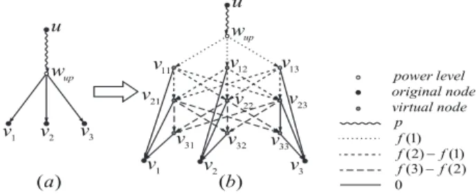
For a power level wup(recall the definition in Section 5.1) of original vertex u that covers k receiving nodes v1, v₂, . . . , v_k, the construction of the gadget is as follows. First, we create k rows of new vertices, with each row containing k vertices, which, in the sequel, will be referred to as “virtual vertices”.

We denote the vertices in row i as v_i1, v_i2, . . . , v_ik. Second, we add a zero-weight edge from each virtual vertex to its corresponding receiving node (e.g, from v11, v21, . . . , vk1 to v1). Then, for the virtual vertices in two adjacent rows, we insert edges between them such that the subgraph formed by the nodes in each two adjacent rows is a complete bipartite graph. The direction of these edges is from the row with lower index to the row with higher index. And we set the weights of all the edges between row i and row i + 1 as f (i + 1) − f (i).

Finally, we add edges from vp to all the virtual vertices in the first row and set their weights as f (1). An example of the gadget is shown in Figure 4.

(8)

v11 v12 v₁₃ v21 v₂₂ v23

v31 v₃₂ v₃₃

power level original node virtual node

(1)(2) (1) (3) (2) 0

ff f f −f

−

u u

v1 v₂ v₃

p

v1 v₂ v3

wup

( )a ( )b

Fig. 4. Illustration of the gadgets for receiving energy: (a) the original gadget in ConMap without receiving energy for a power level of original vertex u and the nodes v1, v2, v3that u can cover transmitting at power p. (b) the corresponding gadget ConMap creates for this power level of u when considering the receiving energy.

We justify the above construction by proving a similar argument as Lemma 2 in the following lemma.

Lemma 3: For an instance M of DeMEM problem with receiving energy, let M⁰ be the directed Steiner tree instance converted from M by ConMap framework considering the receiving energy. Each feasible transmission scheme in M corresponds to a valid Steiner tree in M⁰, and the energy consumption of the scheme equals to the cost of its corresponding Steiner tree.

Proof: Indeed, for a tuple τ = {uτ, {v1, v2, . . . , vm}, pτ, tτ}, it can be encoded as a subgraph consisting of an edge from the original vertex corresponding to uτto its power level p_τin Lt, edges that form a path traversing one of each receiver node’s corresponding virtual nodes once in the gadget on some row (e.g. v₁₁, v₂₂, . . . , v_mm) and edges from the traversed virtual vertices in the gadget to their corresponding receiver nodes (e.g. (v11, v1), (v22, v2), . . . , (vmm, vm)). It is easy to verify from the weight assignments of the edges that the total weight of this subgraph equals to the energy consumption of the transmission. And also as in the proof of Lemma 2, we add necessary edges between different layers, relating a feasible transmission scheme to a Steiner tree.

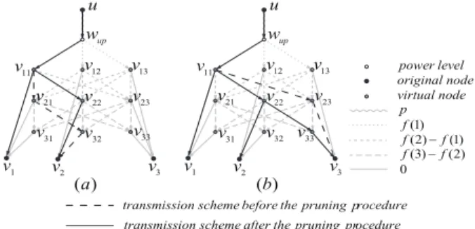
After the computation of a Steiner tree ET in the intermediate graph, however, the existence of the gadgets complicates the pruning process for converting the constructed Steiner tree ET into canonical form. In addition to the pruning procedures mentioned in the previous section, we also need to consider the aberrant phenomena caused by the edges in the gadgets. The pruning process is demonstrated in Figure 5 using two illus- trative cases. Taking Figure 5(b) for example, the constructed Steiner tree entails two receivers v1 and v2 in the transmission but the edges that the algorithm chooses in the gadget are (v₁₁, v₁), (v₁₁, v₂₂), (v₂₂, v₂), (v₁₁, v₂₃), (v₂₃, v₃) instead of the path (v11, v22), (v22, v33) and edges (v11, v1), (v22, v2), (v33, v3), whereas the latter are the ones that correspond to a legitimate transmission scheme. Therefore, we incorporate searching such aberrant subgraphs in the gadgets and correct them to the legitimate ones in the pruning process of the framework. For the Steiner tree ET that ConMap constructs for the intermediate graph, denote g0 as a generic subgraph that lies in the intersection of ET and some gadget. We formally present the pruning procedure for g0 in Algorithm 2. We process all the subgraphs g0 in ET as in Algorithm 2 and finally convert ET to an feasible transmission scheme.

Algorithm 2 Pruning procedure for subgraph g0

Input: An subgraph g0 in the intersection of ET and some gadget

Output: A pruned gadget that is eligible for a Steiner tree in canonical form

1: G := the gadget that g0lies in.

2: {vr1, vr2, . . . , vr_k} := the set of receiving nodes in g0.

3: u, w_up := the transmitting node and the transmitting power level in g0.

4: Delete all the edges except (u, wup) in g0.

5: Add the edge (w_up, v_r₁₁) to g0.

6: Add the set of edges {(v_r₁₁, v_r₂₂), . . . , (v_r_k−1_(k−1), v_r_k_k)}

to g.

7: Add the set of edges {(vr₁1, vr1), . . . , (vr_kk, vr_k)} to g0.

8: return g0

Performance analysis of ConMap with receiving energy:

We summarize the performance guarantee of ConMap with receiving energy in the following theorem.

Theorem 4: For a mobile network with n nodes, let k be the number of destinations and D be the delay constraint. Suppose the directed Steiner tree algorithm embedded in ConMap runs in T (|V |, |E|, k) time and achieves an approximation ratio of g(k) on graph G(V, E). Then in time O(T (Dn⁴, Dn⁵)), ConMap returns a transmission scheme of which the energy cost is less than g(k) times the optimal when the receiving energy is sublinear to the number of receivers and less than

g(k)f (k)

kf (1) times the optimal when the receiving energy is superlinear to the number of receivers.

Proof:Based on Lemma 3, we only need to consider the change of cost of the tree brought by the pruning process.

An important observation of the pruning procedure is that, the edges in the gadget can only move to upper level. Therefore, when f is sublinear, we have f (i + 2) − f (i + 1) ≤ f (i + 1) − f (i) for all i, and it follows that the pruning procedure does not increase the cost of the resulting tree. When f is superlinear, we have f (i + 2) − f (i + 1) ≥ f (i + 1) − f (i) for all i. And as we know f (1) represents the least energy consumption. The consumption after the pruning procedure is f (k). However, before pruning the least energy consumption is kf (1). Hence, in the worst case the pruning procedure increases the cost to a factor of at most _{kf (1)}^{f (k)}. For complexity issues, an m-receiver gadget contains at most m² vertices and m³ edges. Hence, all the gadgets in the intermediate graph contain at most Dn⁴ vertices and Dn⁵ edges. Hence, if we use a Steiner tree algorithm with a time complexity of T (|V |, |E|, k) and an approximation ratio of g(k), our Conmap framework will yield a g(k)-approximation of the optimal transmission scheme for sublinear cost functions and a ^{g(k)f (k)}_{kf (1)} -approximation for superlinear cost functions in a time complexity of O(T (Dn⁴, Dn⁵, k)).

C. An Alternative Gadget Construction

As mentioned in the previous section, ConMap framework increases the approximation ratio of the embedding Steiner tree algorithm by a factor up to _{kf (1)}^{f (k)} when the receiving

(9)

v11 v12 v13

v21 v₂₂ v23

v31 v32 v33

v11 v12 v13

v21 v22 v23

v31 v32 v33

transmission scheme before the pruning procedure transmission scheme after the pruning procedure

u u

power level original node virtual node

(1)(2) (1) (3) (2) 0

ff f f −f

−

v1 v2 v3 v1 v2 v3

wup wup

p

( )b ( )a

Fig. 5. Illustration of two pruning processes of converting the computed Steiner tree in the intermediate graph into canonical form. (a) and (b) are two cases of the conversion.

energy function is superlinear. Therefore, we propose a second method of constructing gadgets in ConMap to capture the receiving energy that can eliminate this factor for superlinear receiving energy functions. The method produces polynomial number of additional nodes when the maximum number of neighbors of a node in the network is logarithmic to the total number of nodes.

The construction works as follows. Starting from the original intermediate graph constructed in Section V, for each power level, we add a new vertex for each possible combi- nation of receiving nodes and refer these vertices as receiving levels. Then, we add edges from each power level to all their corresponding receiving levels and from the receiving levels to all their corresponding receivers. The first set of edges are assigned with weights equal to the receiving energy, i.e, f (k) for a receiving level with k receivers. And the second set of edges are zero-weighted ones.

Now, we justify the validity of the construction. In the gadgets constructed as above, a tuple (u, V⁰, t, p) in a transmission scheme corresponds to a subgraph consisting of an edge from the original vertex associated with u to its power level corresponding to p in Lt, an edge from the aforementioned power level to the receiving level corresponding to V⁰ as the intended receivers and edges from the receiving level to all the vertices associated with nodes in V⁰at time slot t. For the pruning procedure, apart from the first one mentioned in the previous section, we also need to guarantee that the receiving levels included in the computed Steiner tree is connected to all its receivers. If not, we can replace this receiving level with the receiving level that corresponds to the set of connected receivers only. This, again, will not increase the cost of the resulting Steiner tree, and thereby the approximation ratio can be preserved.

In terms of the time complexity of the framework, suppose the embedded Steiner tree algorithm runs in T (|V |, |E|, k) time. In this case, the number of additional vertices in a gadget is of the order O(∆²) (∆ is the degree of the original vertex u). Hence, the total time complexity of ConMap that adopts this alternative gadget construction method becomes O(Γ(∆²Dn², ∆²Dn³)). Therefore, this method is suitable for implementation only when the maximum degree of a node is no larger than logarithmic to the total number of nodes in the network. An example of this alternative construction is illustrated in Figure 6.

D. Impact of Mobility Prediction

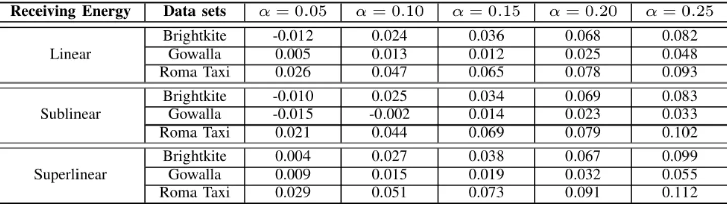
In this section, we briefly discuss the impact of the accuracy of future mobility prediction on the performance of ConMap from a theoretical perspective. We will characterize this impact empirically in Section VII-E. As assumed previously, the theoretical guarantees of ConMap are derived on the basis of perfect future mobility prediction. Now suppose that the mobility prediction we are able to make has an accuracy of 1 − α, i.e., for each edge e = (u, v) in some Gt, it satisfies that (1 − α)w^∗_e ≤ we ≤ (1 + α)w_e^∗, where w_e^∗ is the true value of the weight of e. We subsequently prove that, based on this inaccurate prediction of future mobility, the degradation of ConMap will be no larger than a factor of

1

1−α, which demonstrates the robustness of ConMap against mobility prediction errors.

Let π₀ denote the optimal transmission scheme in the (1 − α)-accurate network and π^∗ denote the optimal transmission scheme in the true network. A straightforward observation is that the inaccuracy of the mobility prediction only has influence on transmitting energy optimization. Denote E as the energy consumption function in the true network and E⁰ as the energy consumption function in the inaccurate network.

Since _1+α¹ we≤ w^∗_e≤ _1−α¹ we, we have E⁰(π^∗) ≤_1−α¹ E(π^∗).

By the optimality of π^∗in the inaccurate network we also have E⁰(π0) ≤ E⁰(π^∗). It follows that E⁰(π0) ≤ _1−α¹ E(π^∗). Hence, if ConMap is guaranteed to find a transmission scheme that is less than β times the optimal one in the inaccurate network we possess, then the transmission scheme it finds is also within

β

1−α of the optimal transmission scheme in the true network, where the energy consumption is calculated with respect to the true network.

power level original node receiving level

(1)(2) 0(3)

ff f

v

1

v

₂

v

₃

u

1, ,2 3

p p p

p

1

p

₂

p

₃

1

w

u

w

_u₂

w

_u₃

Fig. 6. An alternative construction of receiving gadgets.

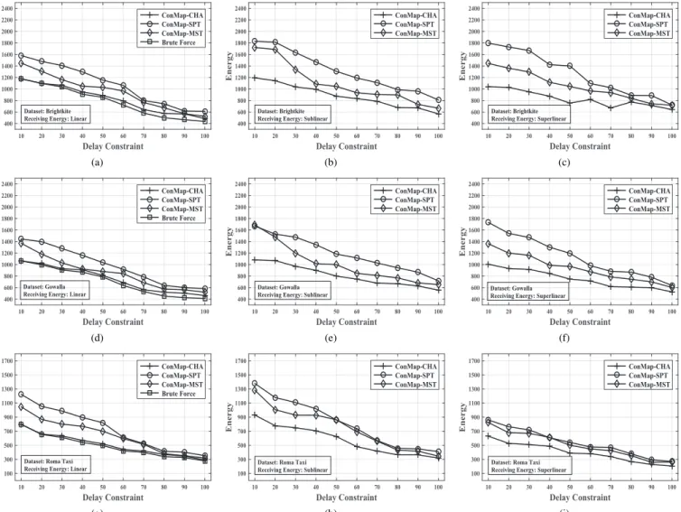
VII. EXPERIMENTS

In this section, we empirically evaluate the performance of ConMap framework. We discuss our experimental settings in Section VII-A and present detailed empirical results in subsequent sections.

A. Experimental Setup

We validate the effectiveness of our ConMap framework based on three real datasets. The basic descriptions of the three data sets are presented as follows.

• Brightkite Social Network [38]: Brightkite is a location- based networking service provider where users share their locations by checking-in. We consider the users