以系統層級動態研析吳郭魚暴露於擾動金屬濃度之生態生理反應

國立臺灣大學生農學院生物環境系統工程學系 博士論文

Department of Bioenvironmental Systems Engineering College of Bio-Resources and Agriculture

National Taiwan University Doctoral Dissertation

以系統層級動態研析吳郭魚

暴露於擾動金屬濃度之生態生理反應 Systems-level dynamics to quantify ecophysiological responses for tilapia Oreochromis

mossambicus exposed to fluctuating metals

陳韋妤 Chen Wei-Yu

指導教授: 廖中明 博士 Advisor: Liao Chung-Min, Ph.D.

中華民國一○○年七月

July, 2011

II

Where the mind is without fear Where knowledge is free

Where words come out from the depth of truth

Where tireless striving stretches its arms towards perfection

Where the mind is led forward by thee into ever-widening though and action—

Into that heaven of freedom, my advisor let my idea awake.

Revised from GiTanJiali by Tagore

2007 9 28

Framework

?

?

?

BLM BLM

BLM !

2009

III

(Vivian璇

IV

Berry

MIT

V

VI

ABSTRACT

Fluctuation exposure of contaminant is ubiquitous in aquatic environments.

Traditional standard laboratory toxicity tests were performed at constant exposure scenarios typically did not elucidate the short-term pulsed exposure toxicity to aquatic organisms. Little is known about copper (Cu) and arsenic (As) toxic effects with pulsed and fluctuation exposures on aquatic organisms. The purpose of this dissertation was to develop a quantitative systems-level approach utilizing toxicokinetics, toxicodynamics, bioavailability, and bioenergetics mechanisms to elucidate the ecophysiological response of tilapia (Oreochromis mossambicus) to fluctuating or sequential pulse Cu and As stresses. This study investigated the relationship among bioavailable metal, accumulative concentration and critical damage level induced growth toxicity for tilapia based on biotic ligand model (BLM), threshold damage model (TDM), and ontogenetic growth-based dynamic energy budgets in toxicology (DEBtox) model.

This study conducted the sequential pulsed Cu exposure bioassays on tilapia population to provide Cu acute/chronic toxicokinetics information. The 10-day and 28-day sequential pulsed Cu exposure experiments were conducted to obtain the bioconcentration factor (BCF) for tilapia population. This study linked bioavailability and bioaccumulation mechanisms to estimate the time and water chemistry dependent BCF. This also study analyzed the As exposure experimental data and pulsed Cu exposure bioassays of tilapia with growth inhibition response by using the proposed systems-level mechanistic model with periodic pulses and fluctuating exposures to simulate and compare the outputs. The ontogenetic growth-based DEBtox model was used to estimate growth coefficient (A0) based on chronic growth bioassay, for assessing Cu and As chronic growth toxicities to tilapia.

VII

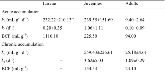
The experimental results indicated that larvae had the highest BCF of 1116.10 mL g^-1 that was greater than those of juveniles 225.50 mL g^-1 and adults 94.00 mL g^-1 in acute pulsed Cu exposure, whereas juveniles had the highest BCF 154.54 mL g^-1 than that of adults 23.10 mL g^-1 in chronic pulsed Cu exposure. Besides, tilapia had a higher Cu accumulation capacity than that of As (BCF=2.89 mL g^-1). Results also showed that BCF value depended significantly on water chemistry conditions and ions concentration. Moreover, BCF value decreased with the increasing of exposure duration. This study also found that tilapia in response to low-frequency Cu/As pulsed exposure had longer 50% safe probability time (ST50) than that of high-frequency pulsed exposure, whereas the longer ST50 was found in high frequency for Cu/As fluctuating exposure. The results indicated that the regulations were triggered between the pulsed intervals. The accumulation of the second Cu pulsed exposure was positively influenced by first Cu pulsed exposure that was consistent with the results of model simulation. The growth coefficients were estimated to be 0.029± 0.0015 g^1/4 d^-1 (Mean±SE) for control and 0.019±0.0017 g^1/4 d^-1 for pulsed Cu exposures in tilapia.

The results indicated that growth coefficient depends positively on the exposure concentrations, revealing that Cu concentration inhibited growth energy and affected the growth of tilapia. The estimated dimensionless mass ratio revealed that sequential and fluctuating Cu exposure could increase tilapia energy acquisition than that of sequential and fluctuating As exposure for overcoming externally fluctuation-driven environments.

This study showed that the dynamics of physiological responses were dependent on the pulsed and fluctuating concentrations, duration, frequency, and different chemical exposure characters in tilapia. Moreover, the time and ions-dependent BCF provided a tool to assess the relationship between accumulation and toxic effect in the

VIII

field situation. We anticipated that this study could provide a completed quantitative systems-level dynamic approach for understating the ecophysiological response of aquatic organisms in response to metal stresses in the field situations. We also hoped that the proposed dynamics of ecophysiological response mechanistic model could successfully assess the long-term metal exposure risk for tilapia population in the field situation of metal exposure impact.

Keywords: Arsenic; Copper; Tilapia; Bioaccumulation; Bioavailability;

Bioenergetics ; Pulsed/fluctuating exposure toxicity; Systems-level

IX

(Oreochromis mossambicus)

(biotic ligand model, BLM) (threshold damage model)

(dynamic energy budgets in toxicology, DEBtox)

10 28

(bioconcentration factor, BCF)

(A0)

1116.10 mL g^-1 225.50 mL g^-1 94.00 mL g^-1

BCF 154.54 mL g^-1 23.10 mL g^-1

X

(BCF=94 mL g^-1) (BCF=2.89 mL g^-1)

50% (ST50)

50%

A0 0.029± 0.0015 g^1/4 d^-1 ( ± )，

A0 0.019±0.0017 g^1/4 d^-1。

/

XI

TABLE OF CONTENTS

I

II

ABSTRACT VI

IX

TABLE OF CONTENTS XI

LIST OF TABLES XIV

LIST OF FIGURES XV

NOMENCLATURE XX

CHAPTER 1. INTRODUCTION 1

CHAPTER 2. BACKGROUND AND RESEARCH OBJECTIVES 2

2.1. Background 2

2.2. Research Objectives 6

CHAPTER 3. LITERATURE REVIEW 7

3.1. Ecologically Relevant Metal Exposure Pattern 7

3.2. Metal Toxic Effects in Aquatic Ecosystems 11

3.2.1. Cu toxicity 11

3.2.2. As toxicity 15

3.3. Mathematical Models 18

3.3.1. Toxicokinetic model 18

3.3.2. Toxicodynamic model 21

3.3.3. Biotic ligand model 25

3.3.4. Threshold damage model 29

3.3.5. West growth model 31

XII

CHAPTER 4. MATERIALS AND METHODS 35

4.1. Pulsed Cu Exposure Experiments 35

4.1.1. Acute accumulation exposure bioassay 35

4.1.2. Chronic accumulation exposure bioassay 39

4.1.3. Chronic growth bioassay 41

4.1.4. Chemical analysis 43

4.2. Data Reanalyses 44

4.2.1. As-tilapia system 44

4.2.1.1. Exposure data 44

4.2.1.2. Chronic toxicity data 46

4.3. Model Development 49

4.3.1. Modeling sequential pulsed and fluctuating exposure patterns 50 4.3.2. Water chemistry-based toxicokinetic/toxicodynamic model 53

4.3.2.1. Water chemistry 53

4.3.2.2. Threshold damage model 55

4.3.3. BLM-based toxicokinetic/toxicodynamic model 57

4.3.4. Ontogenetic growth-based DEBtox model 61

CHAPTER 5. RESULTS AND DISCUSSION 63

5.1. Sequential Pulsed Cu Toxic Effect on Tilapia 63

5.1.1. Acute/chronic toxicokinetic parameters 63

5.1.2. Cu chronic growth toxicity 69

5.1.3. Bioavailability and bioaccumulation of Cu 73 5.1.4. Internal effects with different Cu exposure patterns 79 5.1.4.1. Dynamic effect of sequential pulsed exposure 79 5.1.4.2. Dynamic effect of fluctuating exposure 86

XIII

5.1.5. Ontogenetic growth toxicity of Cu 93

5.2. Sequential Pulsed As Toxic Effect on Tilapia 100

5.2.1. Parameter estimates 100

5.2.1.1. Bioaccumulation factor 100

5.2.1.2. External median effect concentration (EC50) 102

5.2.1.3. Model prediction of EC50(t) data 104

5.2.2. Internal effects with different As exposure patterns 107 5.2.2.1. Dynamic effect of sequential pulsed exposure 107 5.2.2.2. Dynamic effect of fluctuating exposure 114

5.2.3. Ontogenetic growth toxicity of As 120

5.3. Discussion 124

CHAPTER 6. CONCLUSIONS 132

CHAPTER 7. SUGGESTIONS FOR FUTURE RESEARCHES 135

BIBLIOGRAPHY 137

CURRICULUM VITAE 153

XIV

LIST OF TABLES

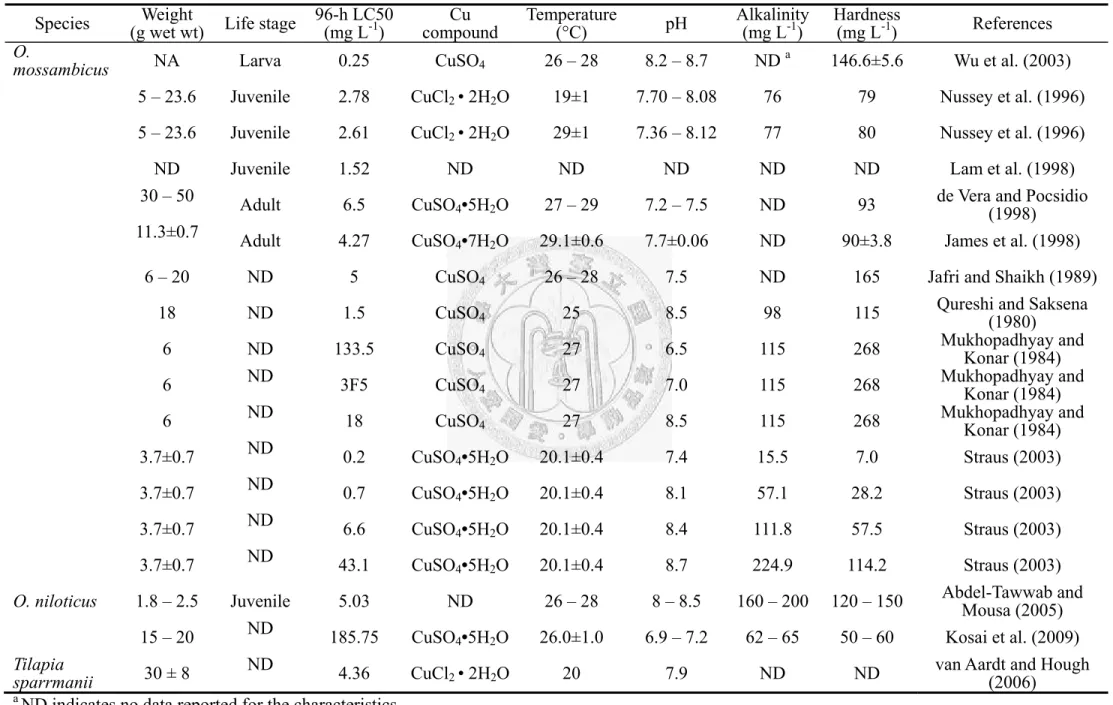
Table 3.1. 96-h median lethal concentration (LC50) of Cu compound and exposure condition on tilapia species

13

Table 3.2. Global As contamination in aquatic systems 17 Table 5.1. Parameter estimates of acute/chronic pulsed Cu-tilapia system for

bioaccumulation model

68

Table 5.2. Point values and distribution of stability constant (log K, M^-1) used in Cu-tilapia system

75

Table 5.3. Parameter estimates of As-tilapia system for bioaccumulation and damage assessment models

106

Table 5.4. Recovery time estimates (mean with 95% CI) for tilapia after sequential pulsed and fluctuating Cu and As exposures

127

Table 5.5. Site-specific temperament, pH, and water chemistry characteristics

from published measured ion concentrations in Hsinchu, Yilan, Hualien, and Tainan area

130

XV

LIST OF FIGURES

Fig. 2.1. A conceptual framework revealing the interaction among experimental data, ecologically relevant exposure pattern, toxicologically mechanistic models, ecophysiologcal response models, and evaluating the environmental risk assessment

5

Fig. 3.1. (A) Relationship among temperature, pH, and As in Clark Fork River. (B) Relationship among temperature, pH, Cd, and Zn in High Ore Creek, Montana, USA. Shaded area denote night time hours

9

Fig. 3.2. Relationship between the time-dependent Zn exposure concentration and survival percentage of cutthroat trout

10

Fig. 3.3. Relationship among (A) waterborne Cu concentration, (B) organ-specific Cu concentration and (C) bioaccumulation factor of tilapia with seasonal variation in Lake Qarun, Egypt

14

Fig. 3.4. Schematic presentation of an one-compartment toxicokinetic model 20 Fig. 3.5. Schematic presentation of toxicodynamic model 23

Fig. 3.6. Hill-based concentration-effect model 24

Fig. 3.7. Schematic representation of the biotic ligand model for metal bioavailability where DOC: dissolved organic carbon and POC:

particular organic carbon

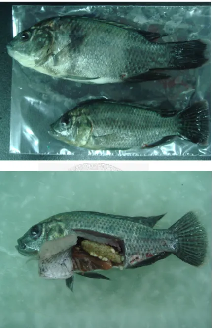
28

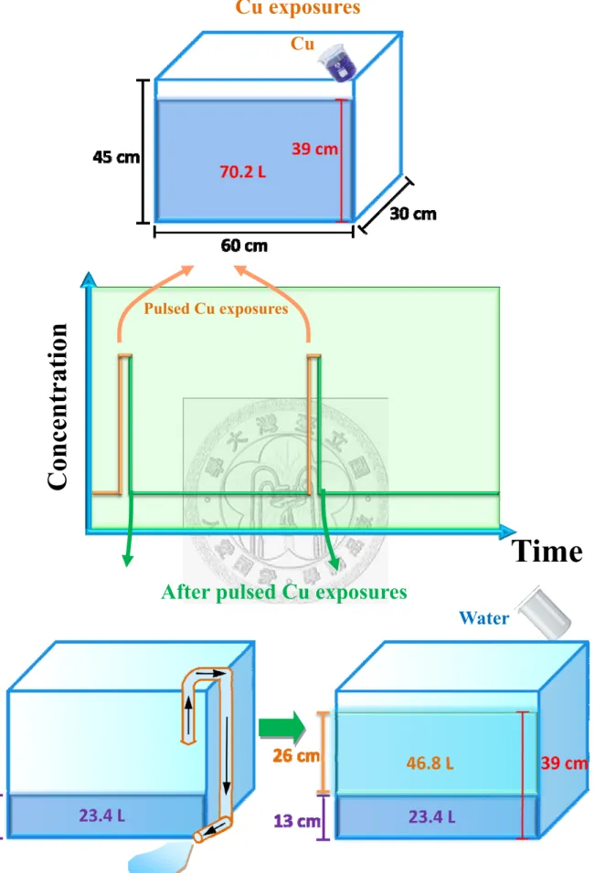
Fig. 4.1. Fish samples used in the Cu-tilapia pulsed exposure bioassay 37 Fig. 4.2. Changes of Cu concentration to achieve the sequential pulsed

exposure

38

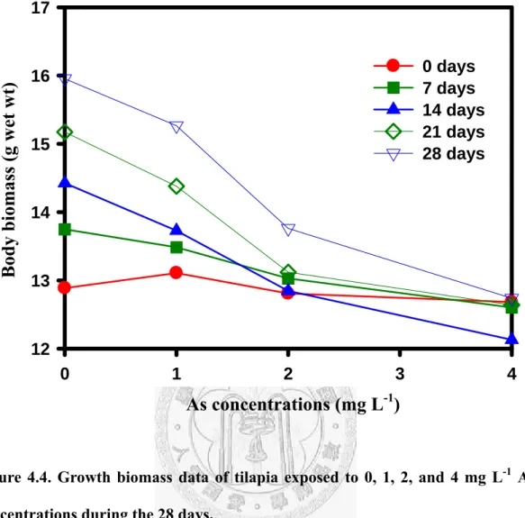
Fig. 4.3. As accumulation concentration by tilapia exposed to 1 mg L^-1 waterborne As for 7 days. Errors bars are standard deviation from mean

45

XVI

Fig. 4.4. Growth biomass data of tilapia exposed to 0, 1, 2, and 4 mg L^-1 As concentrations during the 28 days

48

Fig. 4.5. Diagram of (A) the sequential pulsed waterborne metal exposure pattern and (B) the fluctuating waterborne metal exposure pattern

52

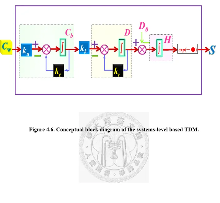
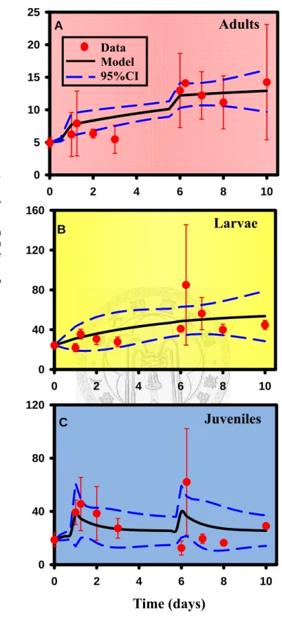
Fig. 4.6. Conceptual block diagram of the systems-level TDM 60 Fig. 5.1. Best-fitting regression curves of acute Cu accumulation to (A) adult,

(B) larval, and (C) juvenile tilapia from first-order bioaccumulation model. Error bars are standard deviation from mean

64

Fig. 5.2. Best-fitting regression curves of chronic Cu accumulation to (A) juvenile and (B) adult tilapia from first-order bioaccumulation model. Error bars are standard deviation from mean

67

Fig. 5.3. The calculated daily growth rate of adult tilapia with/without pulsed Cu exposure during 28 day bioassays

70

Fig. 5.4. Best-fitting regression curves of pulsed Cu damage to tilapia from first-order damage model

71

Fig. 5.5. Using the estimated toxicokinetic and toxicodynamic parameters to predict DAM-based EC50 in adult tilapia

74

Fig. 5.6. (A) Predicted time-dependent f_CuBL^50% by the best-fitting model to estimate (B) BLM-based EC50

76

Fig. 5.7. (A) Using DAM to fit BLM-based EC50 to estimate DAM parameters. (B) The time series of BLM-based bioconcentration factor predicted by Eq. (4.22)

78

Fig. 5.8. Simulations of the sequential pulsed Cu exposure with 5 days pulse periods (left), and 0.5 and 25 days pulse periods (right) for tilapia.

(A, B) Sequential pulsed Cu activity range from 0.0013 – 0.0278 mg

81

XVII

L^-1. (C, D) Body burdens. (E, F) Time course of the damage. (G, H) Hazard rate. (I, J) Cumulative hazard. (K, L) Safe probabilities Fig. 5.9. Simulations of the sequential pulsed Cu exposure with 5 days pulse

periods (left), and 0.5 and 25 days pulse periods (right) for tilapia.

(A, B) Sequential pulsed Cu activity range from 0.0013 – 0.2664 mg L^-1. (C, D) Body burdens. (E, F) Time course of the damage. (G, H) Hazard rate. (I, J) Cumulative hazard. (K, L) Safe probabilities

84

Fig. 5.10. Simulations of the sine-wave Cu exposure with 3 days (left) and 15

days periods (right) for tilapia. (A, B) Sine-wave Cu activity range from 0.0013 – 0.0067 mg L^-1. (C, D) Body burdens. (E, F) Time course of the damage. (G, H) Hazard rate. (I, J) Cumulative hazard.

(K, L) Safe probabilities

88

Fig. 5.11. Simulations of the sine-wave Cu exposure with 3 days (left) and 15

days periods (right) for tilapia. (A, B) Sine-wave Cu activity range from 0.0013 – 0.0265 mg L^-1. (C, D) Body burdens. (E, F) Time course of the damage. (G, H) Hazard rate. (I, J) Cumulative hazard.

(K, L) Safe probabilities

91

Fig. 5.12. Best-fitting regression curves of body biomass to tilapia in (A) control and (B) pulsed Cu exposure groups

94

Fig. 5.13. The time series of the body biomass of tilapia with the (A) sequential pulsed and (B) sine-wave Cu patterns

97

Fig. 5.14. A plot of the dimensionless mass ratio for tilapia with the (A) sequential pulsed and (B) sine-wave Cu patterns

99

Fig. 5.15. Best-fitting regression curves of As accumulation to tilapia from first-order bioaccumulation model. Error bars are standard deviation

101

XVIII

from mean.

Fig. 5.16. Prediction of dose-response profiles of tilapia, Hill based model fit

to measured data varied by different integrated response time of (A) day 1, (B) day 2, (C) day 3, and (D) day 4, respectively

103

Fig. 5.17. Fitting proposed DAM-EC50 equation to experimental EC50(t) data for tilapia

105

Fig. 5.18. Simulations of the sequential pulsed As exposure with 5 days pulse

periods (left), and 0.5 and 25 days pulse periods (right) for tilapia.

(A, B) Sequential pulsed As activity range from 0.061 – 1.270 mg L^-1. (C, D) Body burdens. (E, F) Time course of the damage. (G, H) Hazard rate. (I, J) Cumulative hazard. (K, L) Safe probabilities

109

Fig. 5.19. Simulations of the sequential pulsed As exposure with 5 days pulse

periods (left), and 0.5 and 25 days pulse periods (right) for tilapia.

(A, B) Sequential pulsed As activity range from 0.061 – 11.115 mg L^-1. (C, D) Body burdens. (E, F) Time course of the damage. (G, H) Hazard rate. (I, J) Cumulative hazard. (K, L) Safe probabilities

112

Fig. 5.20. Simulations of the sine-wave As exposure with 3 days (left) and 15

days periods (right) for tilapia. (A, B) Sine-wave As activity range from 0.061 – 0.305 mg L^-1. (C, D) Body burdens. (E, F) Time course of the damage. (G, H) Hazard rate. (I, J) Cumulative hazard.

(K, L) Safe probabilities

116

Fig. 5.21. Simulations of the sine-wave As exposure with 3 days (left) and 15

days periods (right) for tilapia. (A, B) Sine-wave As activity range from 0.061 – 1.215 mg L^-1. (C, D) Body burdens. (E, F) Time course of the damage. (G, H) Hazard rate. (I, J) Cumulative hazard.

118

XIX

(K, L) Safe probabilities

Fig. 5.22. The time series of the body biomass of tilapia with the (A) sequential pulsed and (B) sine-wave As patterns

121

Fig. 5.23. A plot of the dimensionless mass ratio for tilapia with the (A) sequential pulsed and (B) sine-wave As patterns

123

Fig. 5.24. Site-specific ecotoxicological risk assessment of tilapia in Taiwan 131

XX

NOMENCLATURE

[ ] Dissolved ion concentration (g L^-1) {} Free ion activity (M)

A Constants depend on the water permittivity constant and temperature A0 Biological species-specific growth coefficient (g^1/4 d^-1)

AUC Area under the metal concentration in organism versus time curve (µg d g^-1)

[a] {OH } {CO²₃ }

3 3

− + _CuOHBL − + _{CuCOBL CuCO}

CuBL K K K

K (M^-1)

BCF Bioconcentration factor (mL g^-1) BL Biotic ligand (mol g^-1)

BLM Biotic ligand model

C Chemical concentration (mg L^-1)

C0 Background or base line metal concentration (mg L^-1) C1 Pulsed or amplitude metal concentration (mg L^-1) C_b Metal concentration in the body (µg g^-1)

C_e,0 External threshold chemical concentration (mg L^-1) Ci Analytic ion concentration (M)

C_i,0 Internal threshold chemical concentration (µg g^-1) Cw External waterborne metal concentration (mg L^-1)

D Damage (–)

DAM Damage assessment model

DE,50 Damage for 50% effect (–)

D_E,50/k_a Compound equivalent toxic damage level for 50% effect (µg g^-1 d) DEBtox Dynamic energy budgets in toxicology

d Phase without metal exposure (–)

dH Hazard rate (–)

XXI

E Effect elicited by chemical (%) E₀ Initial (background) effect (%)

EC50 Chemical concentration causing the half of maximum effect (%) E_max Maximum effect causing by chemical (%)

Ec0 Metabolic energy required to create a new cell (J)

Ec0 Metabolic energy required to create a new cell in control condition (J) FIAM Free ion activity model

50%

fCuBL Fraction of total number of Cu binding site occupied by Cu at 50% effect

G Growth rate (%)

G₀ Growth rate of fresh body biomass without metal exposure (%) GI Growth inhibition rate (%)

Gm Growth rate of fresh body biomass with metal exposure (%) GSIM Gill surface interaction model

H Cumulative hazard (–)

I Total metal ionic strength (M)

k₃ Proportion between damage and hazard (–) ka Damage accumulation rate (g µg^-1 d^-1) k_e Elimination rate constant (d^-1)

kg,0 Daily growth rate without chemical exposure (% d^-1) k_g,m Daily growth rate with chemical exposure (% d^-1) kk Killing rat constant (g µg^-1 d^-1)

kr Damage recovery rate constant (d^-1) k_u Uptake rate constant (mL g^-1 d^-1)

KMBL Stability constant for the binding of metal to the biotic ligand (M^-1) K_ML Stability constant for the binding of metal to the ligand (M^-1)

XXII

L Ligand (mol g^-1)

LC50 Median lethal concentration (mg L^-1) M⁺ Metal ion concentration (mole L^-1, M)

MBL Metal ion concentration in biotic ligand (mole L^-1, M) ML Metal complex concentration (mole L^-1, M)

MOA Mode of action

m Average resting metabolic rate (J d^-1) m0 Taxon-specific constant (–)

m_c Metabolic rate of a single cell (J d^-1) N Total number of cell in the organims n Hill coefficient (–)

n_i Pulsed frequency of this exposure duration (–) P Permittivity constant (78.3)

r Dimensionless biomass ratio (–) S Safe probability (–)

Scontrol Safe probability resulting from the control effect (–) ST50 50% safe probability time (d)

T Exposure timing or periods (d) TDM Threshold damage model Ts Solution temperature (K)

W Body biomass (g)

W₀ Body biomass at birth (g)

Wi Fresh body biomass at beginning (g) W_c Mass of cell (g)

Wmax Maximum body biomass (g)

XXIII

Wmax0 Maximum body biomass in control group (g) W_t Fresh body biomass at time t (g)

WHAM Windermere humic aqueous model

Z Valence charge number of ion in the solution γ Activity coefficient (–)

δ Dirac delta function

1

CHAPTER 1. INTRODUCTION

For the water quality management in aquatic ecosystems, it is important to be able to predict the impact of metal and toxic effects on aquatic organisms. Traditional standard laboratory toxicity tests are performed at constant exposure scenarios to develop water quality criteria. Yet, fluctuation exposure is ubiquitous in nature.

Aquatic organisms are always exposed to temporal fluctuations of contaminants. In reality, fluctuating/pulsed exposure may be the prevalent form in the field situation (Handy, 1994; Reinert et al., 2002; Nimick et al., 2007). Many factors could affect chemical characteristics, such as wastewater flow, sunshine, rainfall, temperature, and the various effluent ions changed contamination exposure. Hence, incorporating exposure timing and frequency into the realistic exposures to predict the metal toxic effects can improve the robustness of environmental risk assessment.

Fish are commonly used bioindicators for metal contamination due to their sensitivity, wide distribution, abundance, and tolerant to various environmental conditions. Moreover, by including their changes in behaviors, e.g., swimming and avoidance response patterns, it can be measured immediately as responses to the occurrence of contaminants (van der Schalie et al., 2001; Gerhardt et al., 2005, 2006;

Zhou et al, 2008). Behaviors could be used as ecophysiological activity parameters for providing ecological relevance to standard toxicity testing. Consequently, the predictions of ecophysiological mechanisms of aquatic organisms subjected to time-varying exposure patterns may provide a practical implication for species growing, cultivation strategies, and risk assessment in realistic situations.

2

CHAPTER 2. BACKGROUND AND RESEARCH OBJECTIVES 2.1. Background

Arsenic (As) and copper (Cu) are widespread in the environment from anthropogenic and natural processes. As is a hazardous trace element that existing in both organic and inorganic states in the environment. Previous investigations indicated that As could be accumulated in tissues of freshwater organisms.

Consumption of these As contaminated tissues may pose adverse health risk (Williams et al., 2006). It is known that As inhibits more than 200 enzymes and causes adverse effects, leading to serious disorders to organisms (Abernathy et al., 1999).

There had also been serious Cu pollution caused by electroplating industrial discharges in Erhjen River and by computer-related high-tech industrial wastewater in Sien San area of Taiwan, known as green oyster incidents (Lee et al., 1996; Lin and Hsieh, 1999). In addition, copper sulfate (CuSO4) has been widely used to exterminate phytoplankton and control skin lesion of fish in cultured ponds (Carbonell and Tarazona, 1993; Chen and Lin, 2001; Chen et al., 2006). The contamination of various rivers and coastal areas by Cu has been received increasing attention in Taiwan.

Based on previous studies, effluent metal concentration measured in aquatic environment fluctuated with time (Gammons et al., 2005, 2007; Diamond et al., 2005).

Aquatic organisms living in aquatic systems would positively experience pulsed/fluctuating exposures. Water quality standard toxicity tests rely on the exposure magnitude and duration. Typically, standard tests did not investigate the sequential pulsed and fluctuating exposure toxicities to aquatic organisms (USEPA,

3

1995, 2002, 2003). Thus, it is important to be able to predict As and Cu toxic effects with pulsed and fluctuation exposures on aquatic organisms.

Based on the toxicological principles in aquatic ecosystems, the chemical toxicity depends on the external (water chemical) and the internal (biological) factors.

The chemical toxicity was affected by external factors such as temperature, pH, hardness, specific ion levels, and chemical reaction by influencing the mechanisms of the bioavailability to aquatic organisms (De Schamphelaere and Janssen, 2002;

Niyogi and Wood, 2004). Knowledge of the major ion competition and complex effects on chemistry species are quite important. The water chemical mechanistic approach can greatly improve the site-specific ambient water quality criteria for metals. In view of the biological factors, the metal toxicity to aquatic organisms were performed by two phases: (i) metal accumulative capacity through absorption, distribution, metabolism, and excretion (toxicokinetics), and (ii) metal caused adverse effect that acts at the site of action or target site (toxicodynamics).

Farming tilapia (Oreochromis mossambicus) is the most promising aquatic products in Taiwan because of its high market value and is also one of major food sources of human. Therefore, the tolerances of aquatic organism to sequential pulsed As and Cu toxicities are needed to be estimated.

This study presents an integrated methodology and framework to develop a quantitative systems-level modeling approach based on bioavailability and toxicokinetic/toxicodynamic mechanisms to predict ecophysiological responses (i.e.

bioengeretics) of tilapia to sequential pulsed As and Cu concentrations. The overall

4

conceptual framework of this study is illustrated in Fig. 2.1.

Available published experimental database of As-tilapia system together with the proposed Cu-tilapia bioassays could provide an extensive range of physiological characterization including bioaccumulation and ontogenetic growth inhibition response with waterborne metal exposure. This study constructed an integrated model based on toxicologically mechanistic models to develop ecophysiological response model to elucidate ecobehaviors of fish under the ecologically relevant metal exposure patterns.

5

Figure 2.1. A conceptual framework revealing the interaction among experimental data, ecologically relevant exposure pattern, toxicologically mechanistic models, ecophysiologcal response models, and evaluating the environmental risk assessment.

Model Development

Copper/Arsenic to Tilapia Systems

Published Tilapia Data

Ecologically Relevant Exposure Patterns

Fluctuating Exposure Patterns Sequential Pulsed

Exposure Patterns

Toxicologically Mechanistic Models Linkable

BLM

Bioavailability

TDM

Bioaccumulation

Ecophysiological Response Models Ontogenetic Growth-based

DEBtox Model

Environmental Risk Assessment Implications

Arsenic

Tilapia Bioassays

Copper

6

2.2. Research Objectives

Specifically, the major objectives of this study are fivefold:

1. To develop a quantitative systems-level modeling approach to elucidate the ecophysiological response of tilapia to sequential pulsed/fluctuating Cu and As concentrations.

2. To conduct a pulsed Cu acute and chronic exposure experiments to provide information on the toxicokinetics of Cu in tilapia after sequential pulsed exposure patterns.

3. To link the proposed quantitative systems–level modeling approach to bioavailability and bioaccumulation mechanisms for simulating internal effect of tilapia in response to sequential pulsed and fluctuating Cu and As concentrations.

4. To link bioavailability and bioaccumulation mechanisms for simulating bioenergetics of tilapia to sequential pulsed or fluctuating Cu and As concentrations in response to sequential pulsed/fluctuating patterns.

5. To comprise the bioavailability, toxicokinetics, toxicodynamics, and bioenergetics knowledge to illustrate a more reliable prediction for long-term exposure risk assessment in site-specific settings.

7

CHAPTER 3. LITERATURE REVIEW 3.1. Ecologically Relevant Metal Exposure Pattern

In the aquatic ecosystems, the variation in toxicant concentrations can generate either pulsed or fluctuating exposures. The rainfall, accidental spillage of wastes, the periodic emission of anthropogenic contaminants into the waterborne, and precipitations of airborne contaminant can generate pulsed patterns. The metal cycles, pulsed or fluctuating exposure scenarios were dependent on the geology and hydrology (Astruc, 1989; Campbell and Tessier, 1989; Pereira et al., 2009). The diel metal cycles of biogeochemical process are greatly dynamics and short-term (daily and bihourly) variations in metal concentration and speciation (Nagorski et al., 2003;

Authman and Abbas, 2007; Tercier-waeber et al., 2009).

Tercier-waeber et al. (2009) indicated that water chemistry conditions were positively affected by the metal cycles rather than hydrological conditions, the solubility, and availability of metal. The occurrence of diel variations in the As, Cu, and other heavy metal concentrations were found in the surface water (Gammons et al., 2005; 2007; Diamond et al., 2005; Parker et al., 2007; Pereira et al., 2009; 2010).

It is positively confirmed that many factors could affect diel variations in the water chemistry characteristics in As- and Cu-rich aquatic ecosystems. Previous studies indicated the positive relationship between As and pH or temperature (Fig. 3.1A) (Fuller and Davis, 1989; Gammons et al., 2007), whereas the Cd and Zn had negative relationship with pH and temperature (Fig. 3.1B) (Nimick et al., 2007). The Cu concentrations were positively correlated with water flow and dissolved organic carbon (Heier et al., 2010). However, these studies indicated that temperature and pH were the dominant factors for controlling diel fluctuations in water chemistry in the

8

metal-rich stream (Nimick et al., 2003, 2007; Gammons et al., 2005, 2007).

Standard laboratory bioassays carried out the continuous exposure to investigate the chemical induced adverse effect for aquatic organisms that would inaccurately estimate the chemical toxicity and risk (Hoang et al., 2007). Beside, some studies indicated that pulsed/fluctuating exposure toxicity would be induced the latent effect to aquatic organisms (Diamond et al., 2005; Hoang et al., 2007; Nimick et al., 2007).

Nimick et al. (2007) have been conducted the field bioassays to monitor the diel waterborne metal cycle and measure the survival probability for cutthroat trout (Oncorhynchus Clarki Lewisi). Nimick et al. (2007) revealed that the latent mortality and the mortality related prior fluctuating events occurred in the cutthroat trout bioassays (Fig. 3.2). Nimick et al. (2007) suggested that exposure to diel-fluctuating concentration was less toxic than exposure to the constant concentration for cutthroat trout when the average concentration for the fluctuating and a constant was the same.

Moreover, the low concentration periods during the diel cycle would give a sufficient regulating time to repair the gill or tissue damages (McDonald and Wood, 1993;

Reinert et al., 2002; Diamond et al., 2005, 2006; Bearr et al., 2006; Hoang et al., 2007).

9

A

Temperature (°C) Arsenic conc. (μg L-1 ) pH

7 9 11 13

0 10 20 30 40 50

12 18 24 30 36 42

Temp.

As pH

B

Temperature (°C) Cadmium conc. (μg L-1 ) Zinc conc. (μg L -1) pH

Figure 3.1. (A) Relationship among temperature, pH, and As in Clark Fork River (Gammons et al., 2007). (B) Relationship among temperature, pH, Cd, and Zn High Ore Creek, Montana, USA. Shaded area denote night time hours (Nimick et al., 2007).

8.2 8.3 8.4 8.5

6 10 14 18 22 26

30 Temp.

pH

100 300 500 700 900

1 2 3 4 5 6

14 20 26 32 38 44 50 56 62 68 74 Cd Zn

14

14 2 20 8 20 8 2 14 20 2

Time of day (hr)

0 6 12 18 12 18

C

10

200 400 600 800 1000

0 20 40 60 80 100

0 24 48 72 96

Survival Zn

Figure 3.2. Relationship between the time-dependent Zn exposure concentration and survival percentage of cutthroat trout (Nimick et al., 2007).

Zinc conc. (μg L -1)

Survival (%)

Exposure time (hr)

11

3.2. Metal Toxic Effects in Aquatic Ecosystems 3.2.1. Cu toxicity

Numerous researches reported that Cu in fish (Megalops cyprinoids, Chanos chanos, Liza macrolepis, Mugil cephalus, Oreochromis sp) and oyster (Crassostrea gigas) ranged from 0.39 – 1 μg g^-1dry wt and 1.3 – 988 μg g^-1dry wt, respectively (Han et al., 2000; Huang et al., 2001; Chen et al., 2004), whereas the Cu in tilapia ranged from 1.524 – 18 μg g^-1dry wt (Lin et al., 2005a). Copper plays an essential role in cellular metabolism of aquatic organisms (Prasad, 1984; Cousins, 1985).

Several previous studies demonstrated that Cu accumulates in the chloride cell and positively inhibit brachial Na⁺/K⁺-ATPase activities decreasing Na⁺ transport in gill of fish (Li et al., 1998; Grosell and Wood, 2002; Paquin et al., 2002; Wu et al., 2003; De Boeck et al., 2007). That could cause cardiovascular and mortality in fish because the high Cu levels could induce the disruption of branchial ion regulation.

Previous studies have been carried out the acute toxicity and the Cu exposure bioassays to determine the effective Cu concentration of induced mortality and accumulation for tilapia, indicating that the water chemistry and other environmental conditions such as water hardness, humic substance, and pH were positively affected the toxic effect and accumulative capacity (Pelgrom et al., 1995; Nussey et al., 1996;

de Vera and Pocsidio, 1998; James et al., 1998; Straus, 2003; Wu et al., 2003;

Abdel-Tawwab and Mousa, 2005; Naigaga and Kaiser, 2006; van Aardt and Hough, 2006; Kosai et al., 2009). The 96-h median lethal concentration (LC50) of tilapia species from numerous studies were listed in Table 3.1. The rank of waterborne Cu accumulation in organ-specific of tilapia was liver > intestine > kidney > gill (Pelgrom et al., 1995). Generally, the excess Cu was most stored in the liver since it is

12

an important storage organ for aquatic organisms (Buck, 1978; Shearer, 1984).

Authman and Abbas (2007) have measured the seasonal waterborne Cu concentration and organ-specific (gill, muscle, liver) concentration and bioaccumulation factor for tilapia (Tilapia zillii) in Lake Qarun, Egypt. The relationships among waterborne Cu concentration, accumulation concentration, and bioaccumulation factor were found positive (Fig. 3.3). The influential factors included variant temperatures (22.8, 31.2, 30.2, and 19.8 °C), pH (7.8, 8.1, 7.8, and 7.5), and total dissolved solids (19.2, 27.4, 18.7, and 9.3 g L^-1) varied with different seasons.

The hydrological factors with the seasonal variation could affect metal bioavailability and the accumulated metal concentration (Luoma and Rainbow, 2008).

13

Table 3.1. 96-h median lethal concentration (LC50) of Cu compound and exposure condition on tilapia species Species Weight

(g wet wt) Life stage 96-h LC50

(mg L^-1) Cu

compound Temperature

(°C) pH Alkalinity

(mg L^-1) Hardness

(mg L^-1) References O. mossambicus NA Larva 0.25 CuSO4 26 – 28 8.2 – 8.7 ND ^a 146.6±5.6 Wu et al. (2003)

5 – 23.6 Juvenile 2.78 CuCl2 • 2H2O 19±1 7.70 – 8.08 76 79 Nussey et al. (1996) 5 – 23.6 Juvenile 2.61 CuCl2 • 2H2O 29±1 7.36 – 8.12 77 80 Nussey et al. (1996) ND Juvenile 1.52 ND ND ND ND ND Lam et al. (1998)

30 – 50 Adult 6.5 CuSO4•5H2O 27 – 29 7.2 – 7.5 ND 93 de Vera and Pocsidio (1998)

11.3±0.7 Adult 4.27 CuSO4•7H2O 29.1±0.6 7.7±0.06 ND 90±3.8 James et al. (1998)

6 – 20 ND 5 CuSO4 26 – 28 7.5 ND 165 Jafri and Shaikh (1989) 18 ND 1.5 CuSO4 25 8.5 98 115 Qureshi and Saksena

(1980) 6 ND 133.5 CuSO4 27 6.5 115 268 Mukhopadhyay and

Konar (1984) 6 ND 3F5 CuSO4 27 7.0 115 268 Mukhopadhyay and

Konar (1984)

6 ND 18 CuSO4 27 8.5 115 268 Mukhopadhyay and

Konar (1984)

3.7±0.7 ND 0.2 CuSO4•5H2O 20.1±0.4 7.4 15.5 7.0 Straus (2003) 3.7±0.7 ND 0.7 CuSO4•5H2O 20.1±0.4 8.1 57.1 28.2 Straus (2003) 3.7±0.7 ND 6.6 CuSO4•5H2O 20.1±0.4 8.4 111.8 57.5 Straus (2003) 3.7±0.7 ND 43.1 CuSO4•5H2O 20.1±0.4 8.7 224.9 114.2 Straus (2003) O. niloticus 1.8 – 2.5 Juvenile 5.03 ND 26 – 28 8 – 8.5 160 – 200 120 – 150 Abdel-Tawwab and

Mousa (2005) 15 – 20 ND 185.75 CuSO4•5H2O 26.0±1.0 6.9 – 7.2 62 – 65 50 – 60 Kosai et al. (2009) Tilapia

sparrmanii 30 ± 8 ND 4.36 CuCl2 • 2H2O 20 7.9 ND ND van Aardt and Hough

(2006)

a ND indicates no data reported for the characteristics.

14

9.36

12.38

9.84 9.98

5.84

9.2 7.41 8.68

4.92 6.09 5.52 4.74

Spring Summer Autumn Winter Bioaccumulation Factor

Liver Gills Muscle 24.25

36.27

17.71 12.74

15.13

26.95

13.34

10.85

12.75 17.85

9.94 5.93

Body Burden (μg g

)

2.59 2.93

1.8 1.25

Waterborne Copper (mg L

)

Figure 3.3. Relationship among (A) waterborne Cu concentration, (B) organ-specific Cu concentration and (C) bioaccumulation factor of tilapia with seasonal variation in Lake Qarun, Egypt (Authman and Abbas, 2007).

A

B

C

15

3.2.2. As toxicity

Arsenic is a metalloid element naturally occurring in the environment (Duker et al., 2005). As exists in both inorganic and organic forms and four oxidation states, As(III) (arsenite), As(V) (arsenate), As(0) (arsenic), and As(-III) (arsine) in the water, air, and soil, etc. The As toxicity depends on As speciation in that inorganic As species are more toxic than organic ones to the living organisms and As(III) is usually more toxic than As(V) (Goessler and Kuehnett, 2002; Ng, 2005). Neff (1997) indicated that the aquatic ecosystem plays a significant role in the global cycle of As. As concentration is usually less than 2 μg L^-1 in the seawater (Ng and Kinniburgh, 2002;

Ng, 2005). In the unpolluted surface water and groundwater, the average levels of As generally ranged from 1 to 10 μg L^-1, and freshwater varied typically from 0.15–0.45 μg L^-1 (Smedley and Kinniburgh, 2002; Bissen and Frimmel, 2003a, b). The global As contamination in the aquatic system is summarized in the Table 3.2.

Previous investigations indicated that As could accumulate in tissues of aquatic organisms, and humans who consume these As contaminated tissues may pose adverse health risk (Williams et al., 2006). It is known that As leading to serious disorders such as blackfoot disease, skin lesions, and several cancers of bladder, kidney, liver, and vasculature to human (Chen et al., 2005).

Lin et al. (2001, 2005a, b), Huang et al. (2003), Liao et al. (2003), Chen et al.

(2004), Liu et al. (2005, 2007, 2008), and Wang et al. (2007) have conducted a long-term study during 1998–2008 in southwestern Taiwan. The investigations indicated that As concentrations ranged from 40 – 900 μg L^-1 in aquaculture water ponds including farm fish and shellfish, and the dominant As species was inorganic

16

As that % in of total As ranged from 83.6 – 97.9%. Moreover, the As(V) fraction in inorganic As were 84.2 – 100%. Furthermore, As concentrations in fish (tilapia O.

mossambicus and O. sp., milkfish Chanos chanos, Indo-Pacific tarpon Megalopsl cyprinoids, striped mullet Mugil cephalus, and large-scale mullet Liza macrolepis) and shellfish (hard clam Meretrix lusoria and oyster Crassostrea gigas) ranged from 1 – 350 and 4 – 23 g g^-1 dry wt, respectively. Williams et al. (2006) summarized the As concentrations of freshwater fish ranging from 0.13 – 27.45 g g^-1 dry wt in USA.

These indicated that As accumulations in fish in Taiwan were much more than those in USA.

Tsai and Liao (2006) indicated that aquatic organisms continue to accumulate and eliminate As with growth mechanism for the entire life. Liao et al. (2003) also revealed the negative correlations between body weight and As concentration of gill, liver, viscera, stomach, intestine, and muscle for tilapia.

17

Table 3.2 Global As contamination in aquatic systems ^a

Country/region Conc. (μg L^-1) Source Sampling period

Taiwan ^b 10 – 1820 Groundwater NA ^c

Inner Mongolia 1 – 2400 Drinking water 1990s Xinjiang, China 0.05 – 850 Well water 1983 Shanxi, China 0.03 – 1.41 Well water Not stated Bangladesh <10 – >1000 Well water 1996 – 1997 West Bengal, India^b <10 – 3200 Well water NA

Japan 0.001 – 0.293 Natural 1994

Thailand 1 – 5114 Mining waste 1980s – 1994

Vietnam ^b 1 – 3050 Natural NA

Nepal 8 – 2660 Drinking water 2001

Cambodia 1 – 1340 Groundwater 2004 – 2006

Ghana ^b 1 – 175 Anthropogenic, natural NA

Hungary 1 – 174 Deep groundwater 1974

Romania 1 – 176 Drinking water bores 2001 South-west Finland 17 – 980 Well water, natural 1993 –1994 Germany ^b <10 – 150 Natural, mining NA

Spain ^b <1 – 100 Natural NA

United Kingdom ^b <1 – 80 Mining NA

Argentine ^b <1 – 9000 Natural, thermal spring NA Chile 470 – 770 Anthropogenic, natural NA

Mexico 8 – 624 Well water Not stated

Peru 500 Drinking water 1984

Western USA 1 – 48000 Drinking water 1988

a Adopted from Sharma and Sohn (2009).

b Adopted from Nordstrom (2002).

c NA: Not available.

18

3.3. Mathematical Models 3.3.1. Toxicokinetic model

The one-compartment toxicokinetic model depended upon the chemical concentration can be written as (Fig. 3.4),

( )

b

u w e b

dC k C k C t

dt   , (3.1) where Cw is the chemical concentration in the aquatic ecosystem (mg L^-1), Cb is the chemical concentration in aquatic organism (μg g^-1), ku is the uptake rate constant (mL g^-1 d^-1), ke is the elimination rate constant (d^-1), and t is the exposure time (d), respectively.

After the aquatic organism are transferred to clean water, the elimination rate constant can be estimated from the slope of linear regression of log–transformed chemical concentration of tissue in aquatic organism on the elimination phase,

( )

b

e b

dC k C t

dt   . (3.2)

When the steady–state chemical concentration of tissue in the aquatic organism approached (t→∞), Eq. (3.1) can be reduced as,

u

b w

e

C k C

 k  . (3.3)

Under the steady–state condition, the bioconcentration factor (BCF) of aquatic organism and aquatic ecosystem can be calculated from the ratio of the chemical concentration, or the ratio of the uptake rate constant to that the elimination rate constant,

BCF ^u  ^b

e w

k C

k C . (3.4)

19

BCF can be used to quantify chemical accumulation in the tissue of aquatic organism relative to the chemical concentration in the aquatic ecosystem (USEPA, 2003; Luoma and Rainbow, 2005; Fairbrother et al., 2007).

20

Figure 3.4. Schematic presentation of one–compartment toxicokinetic model.

Uptake Elimination

Chemical concentration in aquatic organism (Cb) Chemical concentration in aquatic ecosystem (Cw)

21

3.3.2. Toxicodynamic model

Toxicodynamic model is defined as the toxic processes that the quantitative relationship between the chemical concentration in target sites and the magnitude of the toxic effects for aquatic organisms (Rozman and Doull, 2000; Heinrich-Hirsch, 2001). Toxicodynamic model describes the time-course of chemical action in the target site of the aquatic organism, subsequent physiological impairment that affect the compensatory mechanism, and finally the toxic effect will be emerged at the hazard level of the organism, such as mortality. That could be understood to include all physiological mechanisms through which the chemical concentrations in the blood, plasma, or some tissue cause the increasing intensity of chemical effects (Fig. 3.5).

The concentration-response interaction could be represented as the particular affinity between chemical substance and molecules site of action (i.e., biological receptor). In the previous studies, the characterization of dose–response relationship could be expressed as types of linear and nonlinear models (Bellissant et al., 1998).

Generally, the sigmoid Emax model is commonly used in toxicodynamic model.

Sigmoid Emax model is also referred to as the Hill equation model which was proposed to describe the interaction of the dissociation of oxyhemoglobin (Hill, 1910) (Fig. 3.6),

max

0 50

n

n n

E C

E E

EC C

  

 , (3.5) where Emax is the maximum effect, EC50 is the chemical concentration that causes the half of maximum effect, and n is the slope factor or is referred to as the Hill coefficient which is a measure of cooperactivity. If n > 1 represents positive cooperativity, the relationship is outstanding sigmoid. If n = 1, the mode is hyperbolic

22

and could be expressed another nonlinear equation.

The Hill equation model has been widely applied in the biochemistry, physiology, and pharmacology to investigate the interaction between biological receptor and chemical molecular.

23

Figure 3.5. Schematic presentation of toxicodynamic model.

Toxic action in target site

Physiological response

Increased mortality

24

Figure 3.6. Hill-based concentration–effect model.

Dose n > 1

n < 1

EC50

Effect

Concentration E_max

E0

25

3.3.3. Biotic ligand model

The biotic ligand model (BLM) is a mechanistic model for considering metal bioavailability that has been developed to quantify water chemistry affecting the speciation and bioavailability of chemical in aquatic systems (Paquin et al., 2002;

Niyogi and Wood, 2004; Schwartz and Vigneault, 2007). There is much qualitative evidence indicating that the total metal concentrations are not good predictors of metal bioavailability (Campbell, 1995; Janssen et al., 2003). Specifically, the metal speciation will greatly affect the availability or the bioavailable fraction of chemical to aquatic organisms. The theory of BLM evolved from free ion activity model (FIAM) (Morel, 1983; Campbell, 1995; Brown and Markich, 2000) and gill surface interaction model (GSIM) (Pagenkopf, 1983).

The FIAM concepts describe the variation of toxic effect levels of metal that could be elucidated on the metal speciation and metal interactions with the aquatic organisms. The mechanisms not only take into account the competition among metal ion species and other cations but also consider the binding of free metal ion and metal complexes to the target cellular sites. To induce the biological effects, the metal ion (M) or metal complex (ML) in the external aqueous must be reacted with sensitive site on the biological cellular ligand (BL) of the aquatic organism (Campbell, 1995;

Brown and Markich, 2000; Slaveykova and Wilkinson, 2005), ML

L

M^ ^ ^K^ML , (3.6) [ML] K_ML[M ^] [ L^], (3.7)

MBL BL

M^ ^ ^KMBL , (3.8) {MBL} K_MBL[M ^] { BL^}, (3.9) where [ ] and { } represent the dissolved ion concentration and free ion activity

26

concentrations, respectively. The KML and KMBL are the stability constants for the binding of metal to the ligand and the biotic ligand.

The FIAM indicated that the free metal ions activity is correlated to the toxic effects in aquatic organisms. However, there were still not practically in used and the effects of metal complexation by organic matter were also neglected (Morel, 1983;

Campbell, 1995; Paquin et al., 2002).

The framework of GSIM indicates that pH and alkalinity affect the metal speciation and shows that metal toxicity and availability of fish decreased with increasing hardness and protective cations (Ca²⁺, Mg²⁺) by competition between cationic metals. Besides, the decreasing toxicity levels include the cations binding at the physiologically active gill surface sites since gill membranes could provide the surface capacities of the negative charged proteins to complexes with metal ions and hydrogen ions that within the aquatic organism is associated with acute toxicity (Pagenkopf, 1983).

The GSIM hypothesizes that the respiratory impairment as the criterion of acute toxicity of all metal to fish and the gill surface are capable of forming complexes with metal species and hydrogen ion in the test aquatic environment. Previous studies indicated that acute Cu toxicity had specific inhibitory effects on ion transport functions in fish gill (Wood, 2001; van Heerden et al., 2004). Specifically, Cu toxicity blocked active Na⁺ and Cl^– uptake and transportation in the gills of fish (Laurén and McDonald, 1987; Janes and Playle, 1995). Briefly, the GSIM takes into account the metal binding at target site, stability constant values (binding affinities of free metal

27

and cation and interacting at site of toxic action on the biotic ligand), and the physiological response to the toxicity.

Fig. 3.7 demonstrates BLM framework based on FIAM and GSIM mechanisms.

The toxic effects of metals to aquatic organism depend on water chemical characteristics (such as inorganic composition, organic composition, cation and metal) and physiological mechanism (i.e. acting on the site of action). BLM involves several processes: (i) the metal must first be complexed with organic, inorganic matters and negative biotic ligands inertly during the transport in water that decreases the metal activity, (ii) metal and cation {Ca²⁺, Mg²⁺, Na⁺, H⁺} take together to diffuse to the surface of the aquatic organism with competition interaction that cause diminishing the metal binding to the negative biotic ligand and hence decrease the toxicity, and (iii) the anions (OH , CO )^{ 2}₃^ could be complexed with metal and immediately binding to negative biotic ligands of aquatic organism to invoke the toxic effect. The metal toxic process must first react on biological membrane and following transport in internal toxicity receptor.

The water chemical equilibrium computer program “Windermere humic aqueous model (WHAM)” (Tipping, 1994) can be used to determine metal and ions interactions accounting for the degree of effective chemical binding at the site of action to reflect the toxic effect level.

28

Figure 3.7. Schematic representation of the biotic ligand model for metal bioavailability where DOC: dissolved organic carbon and POC: particular organic carbon.

Biotic ligand (BL)

Inorganic Complexation

Metal

Cation Competition Ca²⁺

Mg²⁺

Na⁺ H⁺

OH^- CO₃^2- HCO₃^- Cl^- SO₄^2- DOC POC Organic Carbon

Complexation

Toxicity Toxicity

29

3.3.4. Threshold damage model

The toxic effect of biological mechanism describes toxic chemical induced-adverse response caused by chemical accumulation within the aquatic organism, indicating that aquatic organism could resist the toxicity invasion and compensates the health. Most methods were used toxicokinetic principle to explore the chemical reactivated the internal adverse effect to aquatic organisms, such as the critical area under the curve and the critical body residue models (Liao et al., 2005;

Tsai et al., 2006). There were some unreasonable assumptions that chemicals could reversible binding in the critical burden residue model and irreversible binding in area under the curve model. Besides, Kooijman and Bedaux (1996) proposed the dynamic energy budget theory that could evaluate the effect of chemical and was referred to as the dynamic energy budgets in toxicology (DEBtox) theory. The DEBtox theory assumes that non-detectable effect of aquatic organisms due to the critical internal chemical does not reach the non-effect threshold.

The internal threshold concentration (Ci,0) links the external threshold concentration (Ce,0) and toxicokinetics (ku, ke), that express asC_i,0 C_e,0k_u /k_e. Hence, the exceeding internal threshold concentration can kill the tissue and causes the hazard to aquatic organisms. The cumulative hazard function is given by,





( )  _{k b}( )

dH t k C t C

dt , (3.10) where the kk is the killing rate constant (g μg^-1 d^-1). However, the DEBtox theory does not include the recovery mechanism. It is only related to the toxicokinetics, not to the toxicodynamics. Hence, Lee et al. (2002) proposed damage assessment model (DAM) that could describe the time course of median effect concentration data for chemicals

30

acting through the reversible interaction between chemicals and receptors. DAM proposes that the hazard occurs based on the irreversible cumulative damage reaching a critical level (Lee et al. 2002).

It could generally illustrate the health state of aquatic organisms with recovery mechanism. The model assumes that chemical accumulates by toxicokinetics of aquatic organisms that could be described by Eq. (3.1). Then the damage accumulation is proportional to the body chemical concentration, and damage recovery is proportional to the cumulative damage (D) that could be expressed as,

( ) _{a b}( ) _r ( ) dD t k C t k D t

dt   , (3.11) where ka is the damage accumulation rate (g μg^-1 d^-1), kr is the damage recovery rate constant (d^-1). Final, the cumulative hazard is proportional to the cumulative damage,

( ) 3 ( )

H t k D t , (3.12)

where k3 is the proportion between damage (D) and hazard (H).

However, there is no critical internal threshold concept in the cumulative hazard function. Ashauer et al. (2007a, b, c) integrated DEBtox theory and DAM to overcome this problem. The refined model was referred to as the threshold damage model (TDM) that have been confirmed to be most suitable mechanism to simulate the survival of aquatic organism after fluctuating and sequential pulsed exposure to chemicals (Ashauer et al., 2007a, b, c, 2010). The TDM includes toxickinetics, reversible-irreversible recovery, toxicodynamics, and critical damage threshold concepts.

31

3.3.5. West growth model

The ecophysiology of aquatic organism has been widely studied and monitored.

Many aquatic organisms such as algae, invertebrates, mussel, and fish are commonly used as bioindicators since their sensitive, the advantage that changes in their behaviors, e.g., swimming, feeding, growth, reproduction, and avoidance response pattern can be measured immediately as responses to the occurrence of contaminants.

This behavior could be used as ecophysiological activity parameters for providing ecological relevance to standard toxicity testing, that is suitable used in online biomonitors (van der Schalie et al., 2001; Gerhardt et al., 2005; 2006). Fishes and bivalves are commonly preferred for biomonitoring in aquatic ecosystems because of wild distribution, abundant, and tolerant to various environmental conditions (Zhou et al., 2008). The body biomass measurement was commonly preferred biomonitoring endpoint of fish for the evaluation of metal in aquatic system. The ecophysiological models of the growth for aquatic organism exposed to contaminant stress had been well developed.

Previous studies have been investigated the allometric scaling relationship between the forms and functions of organism (McMahon, 1973; Feldman and McMahon; 1983; West et al., 1997; West and Brown, 2004). The hypothesized mechanism to explain the pattern of body biomass is based on the allocation of metabolic energy rate between body biomass of maintenance and production (West et al., 1997). Many studies have affirmed that an excess of energy acquisition over maintenance energy requirement, which the relationship between the metabolic rate and body size is the exponent 3/4 (Feldman and McMahon; 1983; Savage et al., 2004;

West and Brown, 2004), whereas some have argued that it is 2/3 based on a simple