Three-dimensional radar imaging of wavy layer and turbulence structures using multiple receivers and multiple frequencies
Jenn-Shyong Chen1, Jun-ichi Furumoto2, Toshitaka Tsuda2, and Mamoru Yamamoto2
1Department of information and Network Communications, Chienkuo Technology University, Taiwan
2 Research Institute for Sustainable Humanosphere, Kyoto University, Japan
Paper submitted to Annales Geophysicae
(2
ndversion)
Corresponding author: Jenn-Shyong Chen
Add.: Department of Information and Network Communications,
Chienkuo Technology University, No. 1, Jieshou N. Rd., Changhua City 500, Taiwan
E-mail: [email protected] Tel : +886–4–7111111 ext 2300 Mobile Phone: +886–9–28128935 Fax: +886–4–7111163
2
4
6
8
10
12
14
16
18
20
22
24
Three-dimensional radar imaging of wavy layer and turbulence structures using multiple receivers and multiple frequencies
Jenn-Shyong Chen1, Jun-ichi Furumoto2, Toshitaka Tsuda2, and Mamoru Yamamoto2
1Department of information and Network Communications, Chienkuo Technology University, Taiwan
2 Research Institute for Sustainable Humanosphere, Kyoto University, Japan
Abstract
The pulsed, beamwidth-limited atmospheric radar suffers from a finite resolution volume, making it difficult to resolve the small-scale irregularity structure of the refractive index (or clear-air turbulence) in the scattering region. Multi-receiver and multi-frequency imaging techniques were thus proposed to improve the spatial resolution of the measurements in the finite resolution volume. The Middle and Upper atmosphere Radar (MUR; 34.85oN, 136.10oN) possesses the capabilities of 5
frequencies, ranging from 46 MHz to 47 MHz, and up to 25 receivers to carry out the imaging techniques. In this paper, we exhibit the three-dimensional (3-D) imaging utilizing 5 frequencies and 19 receivers of the MUR. The Capon method was
employed for the process of imaging, and examinations of a wavy layer and turbulent structures were made, in which the radar beam- and range-weighting effects on the imaging were mitigated beforehand. Information such as echo center and structure morphology in the resolution volume was then extracted after mitigation of both spatial weighting effects. For example, the location distribution of echo centers could imply the traveling orientation of the wavy layer, which was correspondent with horizontal wind direction. Such information of wavy layer structure was more difficult to disclose without removal of the spatial weighting effects. This paper demonstrates an advanced application of 3-D radar imaging to some practical atmospheric phenomena.
Keywords: Interferometry, Instruments and techniques, Turbulence 26
28
30
32
34
36
38
40
42
44
46
48
50
52
54
1. Introduction
Three-dimensional (3-D) radar imaging using multi-receiver and multi-frequency is an advanced technique implemented in the UHF and VHF atmospheric radars to reconstruct the three-dimensional (3-D) structures of refractivity irregularities in the atmosphere (i.e., clear-air turbulence), providing a spatial resolution at meter scale for the irregularity structures in the resolution volume (or the radar volume) [Yu and Palmer, 2001]. There have been several VHF atmospheric radars in the world that can achieve multi-receiver and multi-frequency operations simultaneously, for example, the Middle and Upper atmosphere Radar (MUR) [Hassenpflug et al., 2008], the OSWIN VHF radar [Chen and Zecha, 2009], the Chung-Li VHF radar [Chen et al., 2009], and so on. The latter two, however, have not made a complete
operation/analysis of 3-D radar imaging yet. Recently, the Middle Atmosphere Alomar Radar SYstem (MAARSY) in Norway is another VHF
atmospheric radar which will fulfill multi-receiver and multi-frequency operations in the near future [Latteck et al., 2012]. Among the plentiful studies of radar imaging, Hassenpflug et al. [2008] demonstrated the first use of operational 3-D imaging with five frequencies and nineteen receivers, and illustrated full 3-D views of a Kelvin-Helmholtz billow structure observed by the MUR.
Mostly, the radar echoes received by multi-receiver and multi-frequency were treated separately for 2-D angular structure and for 1-D beam-direction structure, given the terminologies of coherent radar imaging (CRI) [Woodman, 1997; Palmer et al., 1998] and range imaging (RIM) [Palmer et al., 1999] or frequency-domain interferometric imaging (FII) [Luce et al., 2001]. With CRI and/or RIM, there have been plenty of applications to the atmosphere, such as scattering mechanisms and dynamics in polar mesosphere summer echoes (PMSE) [Yu. et al., 2001], small-scale variability of precipitation [Palmer et al., 2006], mitigation of bird contamination [Chen et al., 2007], effect of Kelvin–Helmholtz instability (KHI) on mean vertical wind [Chen et al., 2008], KHI triggered by inertia‐gravity wave [Luce et al., 2008], imaging of equatorial spread F [Chau et al., 2008], clutter suppression [Yu et al., 56
58
60
62
64
66
68
70
72
74
76
78
80
82
84
2010], measurement of aspect sensitivity of refractivity irregularities [Chen and Furumoto, 2013], applications to UHF radar [Chilson et al., 2003] and mobile weather radar [Isom et al., 2013], derivation of horizontal wind velocities [Sureshbabu et al., 2013], and so on.
In the processes of CRI and RIM, however, it is known that the radar beam (or antenna pattern) and range weighting functions of the radar system have spatial weighting effect on the radar echoes. It is thus essential to remove these weighting effects from the imaging results to yield a more applicable imaging map in some circumstances. Nevertheless, removal of these weighting effects using theoretical mathematic forms may result in unrealistic aspect of imaging structure sometimes. To overcome such difficulty, the concept of adjustable weighting function was proposed for RIM [Chen and Zecha, 2009], CRI [Chen and Furumoto, 2011], and 3-D radar imaging [Chen et al., 2011]. Based on the concept of adjustable weighting function and the associated analysis methods in the references, we fulfilled the 3-D imaging of some atmospheric structures to make an advanced application of multi-receiver and multi-frequency technique. In the literature, practical uses of 3-D radar imaging are not many. In view of this, more applications of the 3-D imaging technique to some specific atmosphere phenomena are worth carrying out.
Section 2 reviews the beam- and range-weighting effects on the radar imaging.
Adaptable beam-weighting and range-weighting functions are given briefly for the present study. Section 3 shows the 3-D imaging of a wavy layer and some small-scale variations of echoing structures in the radar volume. In Sect. 4, the atmospheric information extracted from the 3-D imaging structures is discussed. Conclusions are stated in Sect. 5.
2. Observation and spatial weighting effects 2.1 Observations
The radar echoes for 3-D radar imaging were collected by the MUR on 09-10 Feb, 2006. Only the data collected between 20:15-20:25 UT on 9 Feb (05:15-05:25 LT on 10 Feb), 2006, were used for the purpose of this case study. Figure 1 displays the 86
88
90
92
94
96
98
100
102
104
106
108
110
112
114
array configuration of the MUR, where the full antenna array can be partitioned into 25 antenna groups for reception (i.e., the sub-arrays denoted from A1 to F5). In the experiment, the full antenna array was utilized for transmission in vertical, five equally spaced frequencies at 46.00, 46.25, 46.50, 46.75, 47.00 MHz were transmitted sequentially during each pulse, and 21 antenna groups (i.e., receiving channels) were functioned to collect the data of each frequency, respectively. The antenna groups for reception are highlighted in Figure 1, except for the full array which was also used for reception. Inter-pulse-period (IPP) and pulse length were 400 µs and 1 µs,
respectively. The number of coherent integrations was 128, providing a data time resolution of 0.512 s for each transmitter frequency. Sampling time step was 1 µs, giving a range step of 150 m. The sampling range was between 3 km and 22.2 km.
In the process of RIM, the echoes collected from the full antenna array were used.
In the process of CRI, the 19 receiving channels excluding the full array and F1 group were employed (termed as Txfull/Rx1 mode hereafter), which were also used with the multi-frequency data for the 3-D radar imaging. Every 32 data points were used for an estimate of cross-correlation function, giving a time resolution of about 16 s. The Capon method was employed for 3-D radar imaging. Readers can refer to the
appendix for the basic algorithm of 3-D radar imaging. More description of the radar capability can be found in Hassenpflug et al. [2008].
2.2 Equations for beam-weighting effect
In the present experiment, the full antenna array was used for transmission, and the echoes collected from nineteen receivers were applied to CRI. As examined by Chen and Furumoto [2011], the effective beam-weighting function (BWF) suitable for this operational mode (Txfull/Rx1) can be expressed as
2 ) exp(
)
(
222
e
W
, (1)eo 4 2 3
e 10
SNR
c
c eo , (2)
116
118
120
122
124
126
128
130
132
134
136
138
140
142
2 3 T 1 eo c c
, (3)
where W2(θ) is the two-way BWF, θe is the effective beamwidth, SNR is the signal-to- noise ratio of the echoes in dB, and eo indicates the effective beamwidth at infinite SNR. is the variable of angle, and T is the off-beam direction angle (a positive value). The four coefficients, [c1, c2, c3, c4]≒[0.0096, 3.1803, 1.4751, -9.7430], were obtained from fitting processes for the echoes collected by Chen and Furumoto [2011]
with the operational mode Txfull/Rx1. Equations (2)-(3) are empirical, which contain the factors of SNR and T, and may have different forms for various operational modes of the MUR as well as other radar systems. In addition, Eq. (2) is valid for SNR > -10 dB to result in a positive value of e always.
2.3 Equations for range-weighting effect
The range-weighting function (RWF) is a convolution result between the pulse envelope and system impulse response, in which the system impulse response is the inverse Fourier transform of the receiver filter function. Although a theoretical Gaussian RWF is commonly assumed for a rectangular pulse shape with its matched filter [Franke, 1990], some studies have proposed various shapes of RWF for different combinations of pulse shapes and receiver filter functions in the practical process of RIM [Chen and Zecha, 2009]. Chen and Zecha [2009] also contributed the concept of adaptable RWF for improving the continuity of the imaged powers (or brightness) around the boundaries of the sampling gates; such obtained RWF is adaptive to SNR.
A more recent study made by Chen et al. [2013] further proposed an improved RWF that is adaptive to SNR and range within the sampling gate; such kind of RWF could be useful for some practical data analysis, for example, extending the RIM process to a larger range extent for 3-D radar imaging in a sampling gate. To have suitable expressions of adaptable RWF for the present study, we have re-examined the MUR data demonstrated by Chen et al. [2013], and found a set of equations for use, as follows:
144
146
148
150
152
154
156
158
160
162
164
166
168
170
172
) exp(
2 ) exp(
)
(
22 2
2 2
z r
r r r
W
,(4)
zo o zo zo
zo
z σ
SNR
a a
a
σ a
3 3 2 2 11.2 ) 10 (
, (5)
2 3
1 r b
b
σzo , (6)
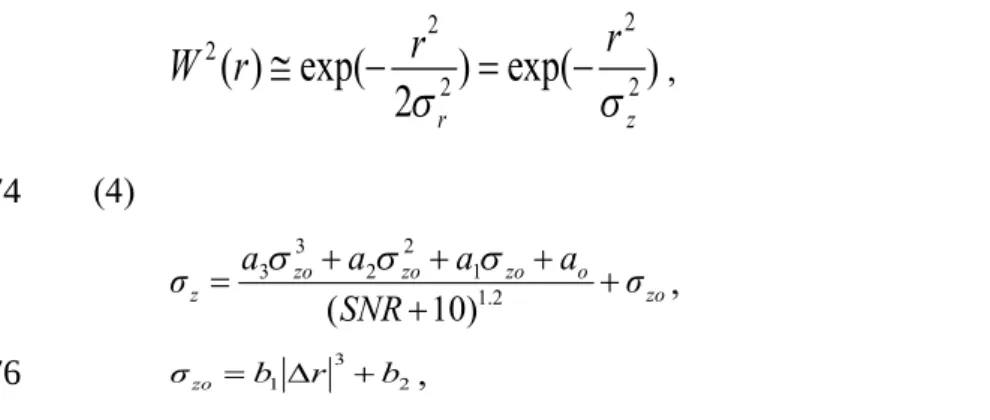
where W2(r) is the two-way RWF, r is the standard deviation of the Gaussian RWF, and z is defined as the effective standard deviation of W2(r) in this paper. SNR is in dB. zo indicates the effective standard deviation of W2(r) at infinite SNR. r is the variable of range, and Δris the off-center range location. The coefficients, [a0, a1, a2, a3]≒[-10742.923, 312.5499, -2.7278, 0.0080723] and [b1, b2]=[1.1457×10⁻⁵, 73.4538], were obtained from fitting processes for the data demonstrated by Chen et al. [2013].
Note again, Eqs. (5)-(6) are empirical, which are adaptive to SNR and r, and may have different forms for various radar parameters as well as other radar systems. In addition, Eq. (5) is valid for SNR > -10 dB. Notice that Eqs. (4)-(6) have the similar forms to Eqs. (1)-(3).
Figure 2 demonstrates the effect of range- and SNR-dependent RWF on a RIM case. For a discussion with wind field later, the time starts from the right side of the abscissa. In the panel (a), the RIM was executed for each sampling gate within the range extent of -75 m to 75 m. The range step of imaging was 1 m and the time resolution was about 16 s. Equations (5) and (6) were employed for correcting the RWF effect of individual sampling gate. As seen, a wavy layer occurred in the sampling gate centered at 5.325 km. The panel (b) is the RIM with the commonly defined RWF (i.e., z=75 m or r53 m) in correction of the imaged power. As seen, the discontinuity of the imaging structure at gate boundaries is more evident than in the panel (a). If the RWF effect is not corrected, the absence of the imaged power occurs at gate boundaries, as observed in the panel (c). Accordingly, we can adopt the range- and SNR-dependent RWF for the present case.
In theory, the imaging process can be extended to the location outside the pulse- 174
176
178
180
182
184
186
188
190
192
194
196
198
200
defined range extent, in case the RWF effect can be compensated thoroughly. In practice, it may not be workable to extend the imaging process too far from the range center. The panels (d)-(f) examined this issue in more detail with the wavy layer in the sampling gate centered at 5.325 km. In the panel (d), the RIM of the wavy layer was performed between -150 m and 150 m only for the sampling gate centered at 5.325 km, and the SNR- and range-dependent RWF was employed. As seen, the obtained wavy layer structure was very close to that in the panel (a). By contrast, the RIM with the commonly defined RWF (i.e., z=75 m or r53 m) in correction of the imaged power is displayed in the panel (e), in which over-correction of the imaged power can be seen around the upper and lower edges of the imaging map. Such an over-
correction of the imaged power can be mitigated but still visible when the SNR- dependent RWF was employed, as shown in the panel (f). In view of this, the RWF adaptive to SNR and range is more suitable for extending the imaging to the locations outside the pulse-defined range extent; it can avoid unexpected change of the imaging structure at gate boundaries and provide a smoother imaging structure through the coverage of a sampling gate. Nevertheless, it should be notified here that the SNR- and range-dependent RWF is not a must for all circumstances. Usually, the SNR- dependent RWF proposed by Chen and Zecha [2009] or Chen et al. [2009] is enough for a normal RIM within the pulse-defined range extent (i.e., -75 m to 75 m for the present experiment).
3 Three-dimensional structure of a wavy layer
For the wavy layer in Fig. 2(d), the 3-D structures at various time slots were examined. Some typical results are shown in Figs. 3 and 5. For clarity of inspection, the contoured angular brightness distributions of nine slices at range locations of -120m, -90m, -60m, -30m, 0m (range center), 30m, 60m, 90m, and 120m are displayed. The unit of the brightness value was dB, but normalization was made for individual time slot. The thick dashed curve in black links the major echo centers at several range locations for convenience of inspection.
In Figs. 3 and 5, two kinds of RIM are also displayed on the range-meridional 202
204
206
208
210
212
214
216
218
220
222
224
226
228
230
plane: one is the sum of the brightness values at equal-range surface (termed as summed-RIM, represented with black solid curve), which is analogous to the
traditional 1-D RIM; the other is the profile of the brightness values at zenith direction (termed as zenith-RIM, indicated by red solid curve), which can suppress the
smearing effect or interference from off-zenith direction. The two kinds of RIM are compared to reveal that the zenith-RIM can provide a thinner layer structure than the summed-RIM via excluding the strong echoes at off-zenith directions. The benefit of zenith-RIM in 3-D radar imaging has been proposed by Hassenpflug et al. [2008] and Yu et al. [2010], for example, suppress the aircraft echoes at off-zenith angles to produce the layer structures with less interference. However, Hassenpflug et al.
[2008] also pointed out that the zenith-RIM from 3-D radar imaging has lower
resolution than 1-D RIM (i.e., retrieved solely from the multi-frequency data collected by the full-array receiving channel and with a vertical radar beam).
In Fig. 3, the time slots numbered 2, 3, and 4 in Fig. 2(d) are displayed, which were around a hump of the wavy layer. Notice that the main body of the wavy layer around the three time slots was located below the range center (see Fig. 2). The panel (a) of Fig. 3 shows the imaging structures without correction of spatial weighting effect (termed original imaging hereafter) at the three time slots, and the panel (b) gives the imaging structures after correction of spatial weighting effect (termed modified imaging hereafter). As observed at the time slot 3, two echo centers can be revealed clearly below the range location of 30 m in the modified imaging; by contrast, the two echo centers cannot be found definitely in the original imaging. On the other hand, the time slots 2 and 4 had the echo centers at opposite zonal directions, which can be disclosed more clearly in the modified imaging. Such features can be explained with the schematic plot of a wavy layer in Fig. 4, in which the time instants t2, t3, and t4 correspond to the time slots 2, 3, and 4 in Fig. 2(d), respectively. At the time instant t3, the echoes may come from both sides of the crest, giving two echo centers at both sides of the zenith in the imaging map. At the time instants t2 or t4, the echoes return mainly from the right or left side of the crest, giving the echo center at positive or negative zenith angle.
232
234
236
238
240
242
244
246
248
250
252
254
256
258
260
More examinations have demonstrated that the 3-D radar imaging can disclose the variation of echo center with range location in the sampling gate. Two more cases at the time slots 12 and 20 are shown in Fig. 5. At the time slot 12, the main echo center was around the range location of -45 m and from positive zonal direction. With increase of range, the echo center shifted to negative zonal direction. Such a variation of echo center with range location can be figured out according to the radar beam location at the time instant t12 in Fig. 4. As illustrated, the body of the wavy layer is very slanted in the illumination volume. The 3-D radar imaging can retrieve such slanted structure in the illumination volume, yielding the imaging map at the time slot 12. By contrast, the body of the wavy layer at the time instant t20 shows an opposite slope to that at the time instant t12, giving the imaging map at the time slot 20 exhibited in Fig. 5.
4 Discussion
In the previous section, we illustrate the capability of 3-D radar imaging for the MUR. Further applications of the imaging results are demonstrated in this section.
4.1 Case 1
The first case is the wavy layer shown in Fig. 2(d). The angular locations of echo centers estimated at nine range locations, i.e., at the nine slices in Fig. 3, are displayed in Fig. 6, where the panel (a) shows the echo centers estimated from the original imaging, and the panel (b) gives the echo centers obtained from the modified imaging.
The method for estimating echo centers is the contour-based approach proposed by Chen et al. (2008).
The echo centers estimated from the modified imaging are supposed to be usable if the spatial weighting effect has been removed properly. However, in Fig. 6 we re- jected the echo center with brightness value lower than 30% of the maximum bright- ness level for raising the reliability of location distribution of echo centers. Moreover, the cases with single and multiple echo centers were displayed separately for a more detailed inspection. In the panel (a) of Fig. 6, the echo centers clustered around zenith, and most of the cases had a single center. After correction of spatial weighting effects, however, plenty of multi-center cases were revealed, as seen in the right-hand plot of the panel (b). In addition, we can observe a northeast-southwest arrangement of echo center locations, in which the echo centers locating at larger off-zenith angles were mostly from multi-center cases.
262
264
266
268
270
272
274
276
278 280 282 284 286 288 290 292 294
The northeast-southwest arrangement of echo center locations can be explained with the morphology of the wavy layer sketched in Fig. 4, assuming the wavy layer travels with a sheared horizontal wind in the northeast direction and the wave shape is slanted to the leeward due to the wind-shear effect. In such circumstance, the wave- front of the wavy layer is in the northwest-southeast direction. For such kind of wavy layer, the radar echoes return mostly from either left or right sides of the crest, result- ing in the location distribution of echo centers in northeast-southwest arrangement.
Moreover, the radar echoes prefer coming from the upstream side of the crest [Chen e al., 2008], i.e., the southwest direction for the present case. This is verified by the val- ues of Zdand Md given in each plot. Zd (or Md) is the difference between the numbers of negative angles and positive angles in zonal (or merid- ional) direction, presented as a percentage of the total number in each plot. Referring to the left-hand plot including single- and multi- center cases for more representative, both values of Zd and Md were apparently above zero no matter in the original or modified 3-D imaging; this implies more echo centers in the lower-left part of the plot and indeed reveals the scenario sketched in Fig. 4.
To validate the above inference, the wind field was examined, as shown in Fig. 7.
For the vertical wind, mean Doppler velocity of 64-point spectrum from the full-array receiving channel was estimated, giving a time resolution of ~32 s. For the horizontal wind, the full correlation analysis (FCA) of spaced antenna [Briggs, 1984] was employed with the data sets of subarrys F5, A4, and B4.
To obtain more reliable wind values from FCA, 512 data points were used, resulting in a time step of about 4.5 min for horizontal wind.
The wind field shown in Fig. 7 has indicated some dynamic motion of the layer structure. As shown, the vertical wind reveals the upward and down- ward motions of the atmosphere, causing the wavy layer structure seen in Fig. 2(d).
On the other hand, the horizontal wind blew toward the northeast direction approxi- mately, which could propel the wavy layer structure to northeast-southwest direction.
Accordingly, the specific location distribution of echo centers in Fig. 6(b) makes sense indeed. Note also the wind shear occurring in the range interval between 5.2 km and 5.4 km, which can deform the wavy layer into that sketched in Figure 4.
It is worth an examination if the above achievement of 3-D radar imaging can be acquired from 2-D radar imaging (CRI) or not. This is illustrated in Fig. 8, where the echo centers obtained from the CRI are shown. Except for the case of single center that was in small number, the locations of echo centers were more scattered than those of 3-D radar imaging, even the BWF effect was mitigated for the CRI (the panel (b)).
296 298 300 302 304 306 308 310 312 314 316 318 320 322 324 326 328 330
pared with Fig. 6. In view of this, the CRI did not disclose the orientation of the wavy layer as clear as the 3-D radar imaging. In addition to the above consequence, we can also observe in the CRI that multiple-center cases were much larger than the single- center cases, which contrasted with the situation of 3-D radar imaging; this is inter- pretable. The CRI is a composite result along the range direction, and so the echoes at different range locations are superimposed for each angular direction. In case more than one scattering centers are located at different directions and range locations, there will be more echo centers in the 2-D angular brightness distribution. In view of this, the benefit of 3-D radar imaging with correction of spatial weighting effects is evident, for this case at least.
4.2 Case 2
The case 1 is a definite wavy layer structure. In Fig. 2(a), we can observe different turbulent structures below ~5 km, which are contrasting with the wavy layer structure.
We examined the echoes in the sampling gate between 4.8 km and 4.95 km for comparison with the first case. The location distribution of echo centers from 3-D radar imaging, like that in Fig. 6, are shown in Fig. 9. Compared with the case of wavy layer, the location distribution of echo centers in Figure 9 were more scattered in both original and modified imaging results, which was mainly due to the scattering distribution of multiple centers shown in the right-hand plots. Such feature seems in consistent with the spatial characteristics of turbulent structures. Another noticeable information is that the values of Zd and Md were positive and comparable to those in Fig. 6, indicating also a favorite direction of southwest for the radar echoes. We can attribute this to the possible slanted structures similar to that sketched in Fig. 4, which could be caused by wind shear effect [Chen et al., 2008]
5 Conclusions
Three-dimensional (3-D) radar imaging using multi-receiver and multi-frequency has been applied to retrieve the atmospheric structure within the radar volume. The observation was carried out with the Middle and Upper atmospheric Radar (MUR).
We have shown the variations of echo centers in the radar volume, verifying the capability of 3-D radar imaging in providing high-resolution structure.
334 336 338 340 342
344
346
348
350
352
354
356
358
360
362
364
To make a more sophisticated study with 3-D radar imaging, our examinations have considered the beam- and range-weighting effects on the radar echoes. Several equations adaptive to off-beam direction, SNR, and range location were used to mitigate the spatial weighting effects for the present radar system and experimental mode. We have demonstrated the benefit of mitigating the spatial weighting effect for a wavy layer structure. For example, the location distribution of echo centers in the radar volume could indicate the traveling direction of the wavy layer structure. This feature of 3-D imaging structure was found to be associated closely with wind field.
In comparison, the above feature of 3-D imaging structure was more difficult to disclose without mitigation of spatial weighting effect, and it could not be found easily from the 2-D radar imaging (CRI) with only multi-receiver echoes. An examination of turbulent structures was also made with the 3-D imaging technique.
Compared with the case of wavy layer, the estimated echo centers were more scattered, conforming with the spatial characteristics of turbulent structures. In addition, in both cases the upstream side of the radar beam (i.e., the southwest direction) was the favorite incident direction of the radar echoes, which is possibly due to the slanted layer/turbulence structures caused by wind shear effect.
The two cases shown in this paper have exhibited some potential applications of 3-D radar imaging implemented in the VHF atmospheric radar. In view of rare publications of 3-D radar imaging in the atmospheric radar community, more studies with the benefit of multi-receiver and multi-frequency technique are worth carrying out in the future.
Appendix A: Equations of 3-D radar imaging
An original and more detailed description of 3-D radar imaging for the atmos- phere can refer to Yu and Palmer [2001], and a simplified introduction was given by Chen et al. [2011]. The following equations are extracted from Chen et al. [2011].
Given N spatially separated receivers at locations of D1, D2,…, Dn and transmit- ting M carrier frequencies at f1, f2,…, fM sequentially during each pulse, the signals from these receivers and carrier frequencies are first expressed as a column vector:
366
368
370
372
374
376
378
380
382
384
386
388
390
392
394
T MN M
M
N N
t S t S t S
t S t S t S
t S t
S t S (t)
)]
( )
( ) (
) ( ...
) ( ) (
) ( ) ( ) ( [
2 1
2 22
21
1 12
11
S
, (A1)
where the superscript T represents the transpose, and Sij(t)is the signal from carrier frequency i and receiver j. The following cross-correlation function of the signal S(t) is required in the imaging process:
MM N M
M M H t
t t
V V V
V V V
V V V S S V
2 1
2 22 21
1 12 11
) ( )(
)(
, (A2)where the superscript H represents the Hermitian (conjugate and transpose) operator.
V(t) is a MN×MN matrix (termed as visibility matrix), and Vpq is a N×N matrix con- sisting of cross-correlation functions between receivers for the frequency pair of p and q. For example,
,
* 2
* 2 2
* 1 2
* 22
* 2 22
* 1 22
* 21
* 2 21
* 1 21
2
MN N M
N M N
MN M
M
MN M
M
M
S S S S S S
S S S
S S S
S S S
S S S
V
(A3)396
398
400
402
404
406
408
where asterisk indicates the conjugate of a complex number. Note that the time vari- able t has been omitted from (A3) for notational simplicity. Vpq is the estimate of visi- bility function without time lag; that is, imaging for different Doppler frequencies of the signals is not made.
The imaging process is to retrieve the so-called brightness distribution via the visibility matrix V, defined as
Vw wH , R , R W
B ( )
) 1
( 2
a a (A4)
where a=[sinθsinφ, sinθcosφ, cosθ], which is the angular direction at zenithal angle θ and azimuthal angle φ. The variable R is the range. W(a, R) is the spatial weighting function for the echoes in the radar volume, formed by radar beam and range weight- ing functions. Matrix w is the weighting vector for retrieving the brightness distribu- tion, given as
T k
R k j k
R k j k
R k j
k R k j k
R k j k
R k j
k R k j k
R k j k
R k j
N M M M
M M
M
N N
e e
e
e e
e
e e
e
]
[
) 2
( )
2 ( ) 2
(
) 2
( )
2 ( ) 2
(
) 2
( )
2 ( ) 2
(
2 1
2 2 2
2 2 1
2 2
1 1 2
1 1 1
1 1
D a D
a D
a
D a D
a D
a
D a D
a D
a
w
,
(A5)
where ki is the wave number of carrier frequency i. Substituting (A5) into (A4) yields the so-called Fourier brightness that has a coarse resolution. To enhance the imaging resolution, the Capon method is one of the choices:
e V e 1
2
1 ) ( ) 1
( H
, R , R W
B a a ,
(A6)
where e has the same form as (A5). Equations (A4) and (A6) indicate that the bright- 410
412
414
416
418
420
422
424
426
428
430
432
434
436
ness value is weighted by the spatial weighting function W(a, R). Removal of W(a, R) from the brightness value is thus necessary to improve the reconstruction of 3-D at- mospheric structure.
Acknowledgements
This work was supported by the National Science Council of ROC (Taiwan), grant no. NSC101-2111-M-270-001 and NSC102-2111-M-270-001. The experiment was supported by the MUR International Collaborative Research Program (Ref. No. 2005- O25), Research Institute for Sustainable Humanosphere, Kyoto University, Japan.
References
Chau, J. L., Hysell, D. L., Kuyeng, K. M., and Galindo, F. R.: Phase cali- bration approaches for radar interferometry and imaging configu- rations:Equatorial spread F results, Ann. Geophys., 26, 2333- 2343, 2008
Chen, J.-S., Hassenpflug, G., and Yamamoto, M.: Tilted refractive-index layers possi- bly caused by Kelvin–Helmholtz instability and their effects on the mean vertical wind observed with multiple-receiver and multiple-frequency imaging techniques, Radio Sci., 43, RS4020, doi:10.1029/2007RS003816, 2008.
Chen, J.-S., and Zecha, M.: Multiple-frequency range imaging using the OSWIN VHF radar: Phase calibration and first results, Radio Sci., 44, RS1010, doi:10.1029/2008RS003916, 2009.
Chen, J.-S., Su, C.-L., and Chu, Y.-H., Hassenpflug, G., and Zecha, M.: Extended ap- plication of a novel phase calibration method of multiple-frequency range imaging to the Chung-Li and MU VHF radars. J. Atmos. and Oceanic Technol., 26, 2488- 2500, 2009.
Chen, J.-S. and Furumoto, J.: A novel approach to mitigation of radar beam weighting effect on coherent radar imaging using VHF atmospheric radar, IEEE Trans.
Geosci. Remote Sens., 49, 3059-3070, doi:10.1109/TGRS.2011.2119374, 2011.
Chen, J.-S., Chen, C.-H., and Furumoto, J.: Radar beam- and range-weighting effects 438
440
442
444
446
448
450
452
454
456
458
460
462
464
466
on three-dimensional radar imaging for the atmosphere. Radio Sci., 46, RS6014, doi:10.1029/2011RS004715, 2011.
Chen, J.-S., and Furumoto, J.: Measurement of atmospheric aspect sensitivity using coherent radar imaging after mitigation of radar beam weighting effect, J. Atmos.
Ocean. Technol., 30, 245–259, doi: 10.1175/JTECH-D-12-00007.1, 2013.
Chen, J.-S., Su, C.-L., Chu, Y.-H., Kuong, R.-M., and Furumoto, J.: Measurement of range-weighting function for range imaging of VHF atmospheric radars using range oversampling technique, paper submitted to J. Atmos. Ocean. Technol.
(accepted after minor editorial revision), 2013.
Chen, M.-Y., Yu, T.-Y., Chu, Y.-H., Brown, W. O. J., and Cohn, S. A.: Application of Capon technique to mitigate bird contamination on a spaced antenna wind pro- filer, Radio Sci., 42, RS6005, doi:10.1029/2006RS003604, 2007.
Chilson, P. B., Yu, T.‐Y., Strauch, R. G., Muschinski, A., and Palmer, R. D.: Imple- mentation and validation of range imaging on a UHF radar wind profiler, J. At- mos. Oceanic Technol., 20, 987–996. 2003.
Franke, S. J.: Pulse compression and frequency domain interferometry with a fre- quencyhopped MST radar, Radio Sci., 25, 565-574. 1990.
Hassenpflug, G., Yamamoto, M., Luce, H., and Fukao, S.: Description and demon- stration of the new Middle and Upper atmosphere Radar imaging system: 1-D, 2- D and 3-D imaging of troposphere and stratosphere, Radio Sci., 43, RS2013, doi:10.1029/2006RS003603, 2008.
Isom, B., Palmer, R. D., Kelley, D, Meier, J., Bodine, D., Yeary, M. Cheong, B.-L., Zhang, Y., Yu, T.-Y., and Biggerstaff, M. I.: The atmospheric imaging radar: si- multaneous volumetric observations using a phased array weather radar. J. Atmos.
Oceanic Technol., 30, 655–675, 2013.
Latteck, R., Singer, W., Rapp, M., Vandepeer, B., Renkwitz, T., Zecha, M., Stober, G.: MAARSY: The new MST radar on Andǿya: System description and first re- sults, Radio Sci., 47, RS1006, doi:10.1029/2011RS004775, 2012.
Luce, H., Yamamoto, M., Fukao, S., Hélal, D., and Crochet, M.: A frequency domain radar interferometric imaging (FII) technique based on high-resolution methods, J.
Atmos. Solar-Terr. Phys., 63, 221–234, 2001.
468
470
472
474
476
478
480
482
484
486
488
490
492
494
496
Luce, H., Hassenpflug, G., Yamamoto, M., Fukao, S., and Sato, K.: High‐resolution observations with MU radar of a KH instability triggered by an inertia‐gravity wave in the upper part of a jet stream, J. Atmos. Sci., 65, 1711–1718, 2008.
Palmer, R. D., Gopalam, S., Yu, T.-Y., and Fukao, S.: Coherent radar imaging using Capon’s method, Radio Sci., 33, 1585-1598, doi:10.1029/98RS02200, 1998.
Palmer, R. D., Yu, T.-Y., and Chilson, P. B.: Range imaging using frequency diver- sity, Radio Sci., 34, 1485–1496, doi:10.1029/1999RS900089, 1999.
Palmer, R. D., Cheong, B. L., Hoffman, M. W., Fraser, S. J., and López-Dekker, F. J.:
Observations of the small-scale variability of precipitation using an imaging radar, J. Atmos. Ocean. Technol., 22, 1122–1137, 2006.
Sureshbabu, V.N. ; Anandan, V.K. ; Tsuda, T. ; Furumoto, J. ; Rao, S.V.: Perfor- mance analysis of optimum tilt angle and beam configuration to derive horizontal wind velocities by postset beam steering technique, IEEE Trans. Geosci. Remote Sens. , 51, 520-526, doi: 10.1109/TGRS.2012.2200256, 2013 .
Woodman, R. F.: Coherent radar imaging: Signal processing and statistical properties, Radio Sci., 32, 2372–2391, doi:10.1029/97RS02017, 1997.
Yu, T.-Y., and Palmer, R. D.: Atmospheric radar imaging using multiple-receiver and multiple-frequency techniques, Radio Sci., 36, 1493-1503,
doi:10.1029/2000RS002622, 2001.
Yu, T.-Y., Palmer, R. D., and Chilson, P. B.: An investigation of scattering mecha- nisms and dynamics in PMSE using coherent radar imaging, J. Atmos. Solar-Terr.
Phys., 63, 1797-1810, 2001.
Yu, T.-Y., Furumoto, J., and Yamamoto, M.: Clutter suppression for high-resolution atmospheric observations using multiple receivers and multiple frequencies, Radio Sci., 45, RS4011, doi:10.1029/2009RS004330, 2010.
498
500
502
504
506
508
510
512
514
516
518
520
522
Figure Captions
Figure 1. Array configuration of the MUR. Twenty-five antenna groups for
transmission/reception are indicated from A1 to F5. The diameter of the array field is about 110 m. The highlighted subarrays, as well as the full array, are employed for reception in the experiment, but the data of F1 subarray are not used in the study.
Figure 2. Range imaging of a wavy layer, observed by the MUR. The range step of imaging is 1 m, and time resolution is about 16 s. The time starts from the right side of the abscissa. (a) Range imaging for six sampling gates with range centers at 4.725km, 4.875km, 5.025 km, 5.175 km, 5.325 km, and 5.475 km, respectively.
Imaging process of each gate is from -75 m to 75 m with respect to the range center of the sampling gate, and SNR- and range-dependent RWF is used in correction of brightness value. (b) and (c) are similar to (a) but with a commonly defined RWF in (b) and without correction of RWF in (c). The three panels of (d)(e)(f) are the imaging results for the sampling gate centered at 5.325 m, but the imaging process is from -150 m to 150 m with respect to the range center of the sampling gate and uses different RWFs in correction of brightness value. The numbers given in the panel (d) denote the time slots.
Figure 3. 3-D radar imaging results at the time slots 4, 3, and 2 (from left to right) indicated in Figure 2(d). The 2-D contoured brightness distributions of nine slices at range locations of -120m, -90m, -60m, -30m, 0 m (range center), 30m, 60m, 90m, and 120m are displayed. The unit of the brightness value is dB, but normalization is made for individual time slot. (a) and (b) are the imaging results, respectively, with and without correction of spatial weighting effect. The thick dashed curve in black links the major echo centers at several range locations. Black spot is the central location of the radar volume. Two types of 1-D RIM profiles are shown on the range-meridional plane: (black) summation of the brightness values at equal-range surface, (red) the brightness values along the zenith direction.
Figure 4. A wavy layer structure in a wind-sheared atmosphere. Radar beam is vertical. tn denotes different observational times corresponding to the time slots 524
526
528
530
532
534
536
538
540
542
544
546
548
550
552
indicated in Fig. 2(d).
Figure 5. Same as Figure 3, but showing the imaging results at the time slots 20 and 12 (from left to right) indicated in Figure 2(d). Correction of spatial weighting effect is made.
Figure 6. Angular locations of echo centers at range locations of -120m, -90m, -60m, -30m, 0m (range center), 30m, 60m, 90m, and 120m in the radar volume for the wavy layer structure. (a) and (b) result from the 3-D imaging, respectively, with and without correction of spatial weighting effect. The left-hand plots show all estimates, and the middle and right-hand plots display the situations of single center and multiple centers, respectively.
Figure 7. (upper) vertical wind estimated from the Doppler spectrum of 64 data points, and (lower) horizontal wind derived from full-correlation analysis of spaced antenna with 512 data points.
Figure 8. Similar to Figure 6, but resulting from the 2-D radar imaging of multi- receiver echoes.
Figure 9. Similar to Figure 6, but obtained from the echoes in the sampling gate between 4.8 km and 4.95 km.
554
556
558
560
562
564
566
568
570
572