3D列印之路徑規劃演算法於三軸氣壓式並聯機構機械臂之研究

(1)

國立臺灣大學工程科學及海洋工程學系碩士論文

Department of Engineering Science and Ocean Engineering College of Engineering

National Taiwan University Master Thesis

3D 列印之路徑規劃演算法

於三軸氣壓式並聯機構機械臂之研究 The Development of Path Planning Algorithm

for 3D Printing

in a Three-Axial Pneumatic Parallel Manipulator

温志培 Chih-Pei Wen

指導教授：江茂雄博士

Advisor: Dr.-Ing. Mao-Hsiung Chiang

中華民國 105 年 1 月

January, 2016

(2)

誌謝

本論文的完成承蒙指導教授江茂雄老師的授業解惑，感謝老師在專業領域上的教導，同時培養具獨立思考及解決問題的能力，讓我收穫良多。老師亦時常分享人生經驗及待人處事的道理，讓我以正面態度面對接下來人生的挑戰。在此，

學生致上最衷心的感謝與祝福。

感謝口試委員郭振華教授、江茂欽教授、黃金川教授，於百忙之中不吝撥冗，

給予本論文提供寶貴的意見與建議，部分見解是學生未曾思考過的問題，非常感謝各位教授，讓本論文更加的完善。

感謝實驗室同窗雲璠、雲傑、喬陽，在這段時間的相互幫助、鼓勵、研究討論，有幸能與你們成為同窗，希冀畢業後仍保持聯絡，延續這難得的緣分。特別感謝學長維新，教導機台的架構與使用方法；特別感謝同窗喬陽，協助模擬軟體的操作與影片錄製；特別感謝學弟俊辰，協助錄製機台的實驗影片。感謝實驗室的學長姐與學弟妹們，在這段時間的幫忙，有幸能認識大家。

感謝求學過程中遇到的同儕，無論僅是課程上分組的組員、舉辦活動的成員，

亦或是已成為摯友，彼此互相砥礪、成長、蛻變，讓我認識到不一樣的自己。感謝求學過程中遇到的長輩，無私分享生活、求學、工作的寶貴經驗，讓我在面臨類似情況時，能更有智慧地去面對。

最後，感謝我摯愛的家人們，父親温春得先生、母親潘美玲女士、弟弟温博修。感謝從小到大的栽培與照顧，在生活與課業上給予最大的支持與鼓勵，讓我順利完成學業，無後顧之憂，有幸能與你們成為家人是我這輩子最幸福的事，在此獻上我最高的謝意。

謹以此論文，獻給我最敬愛的家人、師長及所有關心我的人。

温志培僅誌於台北公館民國一百零五年一月

(3)

中文摘要

本研究旨在發展 3D 列印的軌跡規劃演算法並應用於三軸氣壓式並聯機構機

械臂，置重點於3D 列印的軌跡規劃於三軸氣壓式並聯機構機械臂，結合實驗室已

發展之三軸氣壓式並聯機構機械臂之運動學分析與控制器設計，以模擬及實際實驗驗證。

在 3D 列印的軌跡規劃方面，將欲列印的物體，採用圖論(Graph Theory)的向

量形式建立。透過深度優先搜尋(Depth-First Search, DFS)定義一個平面的所有分歧路徑，並由基因演算法(Genetic Algorithm, GA)計算如何以最低代價連接所有分歧路徑。最後將每個平面的路徑串接，即可得軌跡規劃。

在三軸氣壓式並聯機構機械臂的運動學分析方面，採用幾何向量的理論與空間中向量迴圈的封閉性質，透過逆向與順向運動學的定義分別推導出致動器與運動平台的關係。

在三軸氣壓式並聯機構機械臂的控制器設計方面，單軸氣壓伺服系統採用雙迴圈回授控制策略，其中包含內圈的壓力控制與外圈的位置控制。根據上述方法，

並額外採用逆向動力學控制策略，以實現三軸氣壓式並聯機構機械臂的控制與解決三軸的非線性耦合。

在本論文最後，透過數值模擬，檢測三軸氣壓式並聯機構機械臂之推導模型

與3D 列印之軌跡規劃的正確性。為證明實用性，藉由實驗室已建立之三軸氣壓式

並聯機構機械臂實驗系統的實驗，輸入與數值模擬相同的軌跡，驗證控制器的效

能與3D 列印整合三軸氣壓式並聯機構機械臂的可行性。

關鍵詞：3D 列印、軌跡規劃、深度優先搜尋(DFS)、基因演算法(GA)、氣壓伺服系統、並聯式機構機械臂、運動學分析、軌跡追蹤控制

(4)

ABSTRACT

This study aims to develop 3D-printing path planning algorithms and applies to a three-axial pneumatic parallel manipulator. The emphasis is on the research of 3D-printing path planning algorithms, integrating the three-axial pneumatic parallel manipulator which has developed on its kinematic analysis and controller design in lab before, and verifying the performance through the whole system simulations and experiments.

In path planning algorithms for 3D printing, the desired-printing object was established from graph theory as vector form. From the view of a layer, all sub-paths are defined through the depth-first search, and the genetic algorithm is used to find the minimum costs linking sub-paths. After cascading all layers, the overall path is accomplished.

In analysis of kinematics, the geometric method is introduced to solve the relation of manipulator between actuated joints and moving platform through vector-loop closure equations, including inverse and forward kinematics.

In controller design, control strategy of single-axial pneumatic servo system is applied with dual-loop feedback control scheme, i.e. inner pressure control and outer position control. Based on that, controller of three-axial pneumatic parallel manipulator is established with extra inverse dynamics control strategy to decouple the nonlinear terms.

Finally, numerical simulations are carried out to verify the correctness of the derived models and the path-planning trajectories. To show the practicality, real-time experiments are implemented in the test rig of three-axial pneumatic parallel mechanism

(5)

robot with the same trajectories in simulations for testifying the control performance and the possibility of 3D printing integrating with three-axial pneumatic parallel manipulator.

Keywords: 3D printing, path planning, depth-first search (DFS), genetic algorithm (GA), pneumatic servo system, parallel manipulator, kinematic analysis, path tracking control

(6)

LIST OF FIGURES

Fig. 2.1 Three-axial pyramidal pneumatic parallel manipulator ... 9

Fig. 2.2 Joint-link configuration of the parallel manipulator ... 9

Fig. 2.3 Photograph of the three-axial pyramidal pneumatic parallel manipulator ... 10

Fig. 2.4 Test rig layout of the pneumatic servo positioning system ... 11

Fig. 2.5 Test rig layout of the overall manipulator system ... 13

Fig. 3.1 Slicing a desired printing object equally ... 16

Fig. 3.2 The definition of layers ... 16

Fig. 3.3 Equal-sized rectangular mesh on a layer: (a) front view (b) top view... 17

Fig. 3.4 The position of a point (red dot) substitutes component mesh ... 17

Fig. 3.5 A directed graph with 5 vertices and 5 edges ... 18

Fig. 3.6 Double-directions directed graph on a layer before path planning ... 19

Fig. 3.7 Single-direction directed graph between layers before path planning ... 19

Fig. 3.8 The priorities of traversing directions (1 is the highest priority) ... 21

Fig. 3.9 The linkages between each two points based on traversing directions: (a) 6 points (b) double-directions linking strategy ... 21

Fig. 3.10 A general example of modified-DFS ... 24

Fig. 3.11 The exception in modified-DFS: (a) 11 points (b) some un-traversed points after modified-DFS ... 26

Fig. 3.12 Solution of the exception in modified-DFS: (a) selecting a new start point nearest to the start point of Sub-path 1 (b) using modified-DFS again and checking the counter when completed ... 26 Fig. 3.13 A complete example of modified-DFS including the exception: (a) 45 points

(10)

(b) 4 sub-paths after modified-DFS ... 27

Fig. 3.14 Notations of sub-paths for Genetic Algorithm ... 28

Fig. 3.15 An example of two initial populations ... 29

Fig. 3.16 An example of ideal shortest total lengths ... 29

Fig. 3.17 An example of crossover ... 30

Fig. 3.18 An example of mutation at Sub-path 2 ... 30

Fig. 3.19 An example of the exception in step D (i) ... 32

Fig. 3.20 An example of the exception in step D (ii) ... 32

Fig. 3.21 Solution of the exception at Sub-path 1 in step E ... 32

Fig. 3.22 Path planning on a layer: (a) 9 points (b) planned path trajectory... 33

Fig. 3.23 Layer-to-layer path planning on a 3-layers object ... 34

Fig. 3.24 The exception in layer-to-layer path planning: (a) after single-layer path planning on Layer i (b) a non-existent start point (purple dot) on Layer

1 i +

... 35

Fig. 3.25 Solution of the exception in layer-to-layer path planning: (a) creating the non-existent start point on Layer

i + 1

(b) linking to nearest point and changing the start point on Layer

i + 1

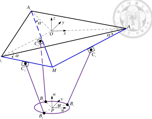
... 35

Fig. 4.1 Schematic diagram of the three-axial pyramidal parallel manipulator ... 37

Fig. 4.2 Geometry of one typical limb ... 37

Fig. 4.3 Vector representation for one typical limb ... 38

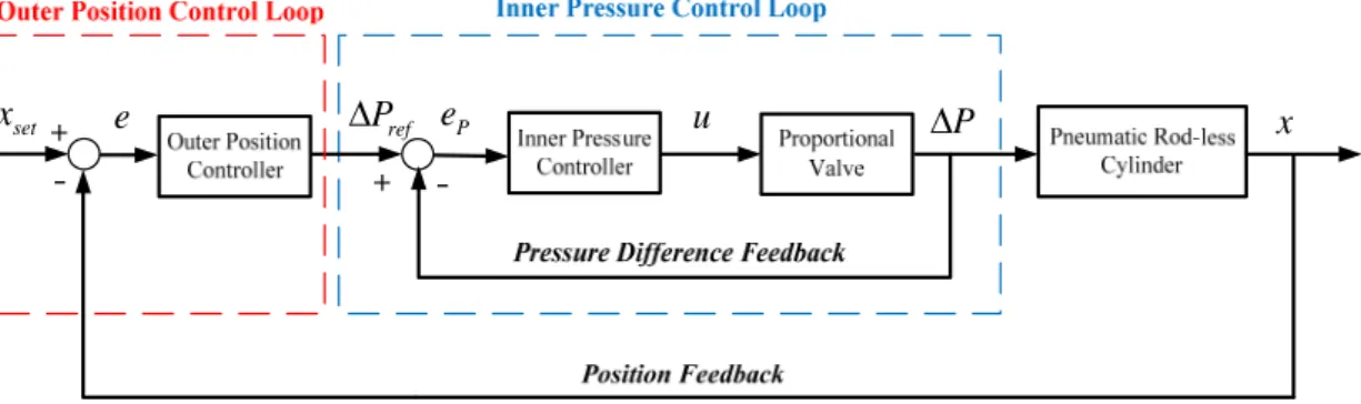
Fig. 5.1 Dual-loop control scheme for position control of the pneumatic cylinder system ... 45

Fig. 5.2 PI control with back-calculation anti-windup method... 46

Fig. 5.3 Schematic diagram of position control of single-axial pneumatic cylinder system ... 46

(11)

Fig. 5.4 Inner-loop control design of inverse dynamics control for the three-axial

pyramidal pneumatic parallel manipulator ... 48

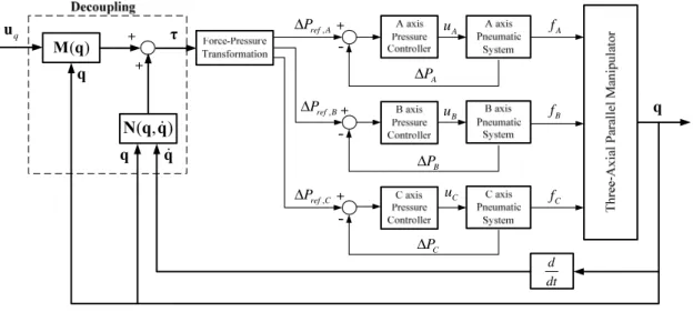
Fig. 5.5 Schematic diagram of inverse dynamics control for the three-axial pyramidal pneumatic parallel manipulator ... 48

Fig. 5.6 Schematic diagram of the overall control system ... 49

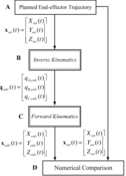
Fig. 6.1 Procedure of model verification for inverse and forward kinematics ... 51

Fig. 6.2 Designed circle-shape line trajectory for end-effector ... 53

Fig. 6.3 Calculated joint space trajectories via inverse kinematics for the circle-shape line trajectory: (a) A-axis actuator (b) B-axis actuator (c) C-axis actuator .. 54

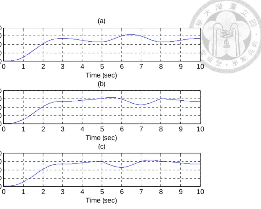
Fig. 6.4 Calculated task space trajectories via forward kinematics for the circle-shape line trajectory: (a) X-axis (b) Y-axis (C) Z-axis ... 54

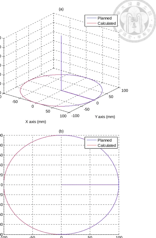
Fig. 6.5 Comparison between the planned and the calculated end-effector for the circle-shape line trajectory: (a) front view (b) top view ... 55

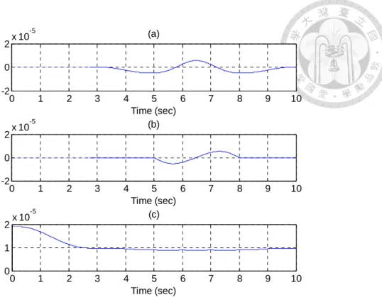
Fig. 6.6 Numerical error between the planned and the calculated end-effector for the circle-shape line trajectory: (a) X-axis (b) Y-axis and (C) Z-axis ... 56

Fig. 6.7 Designed sphere-shape line trajectory for end-effector ... 57

Fig. 6.8 Calculated joint space trajectories via inverse kinematics for the sphere-shape line trajectory: (a) A-axis actuator (b) B-axis actuator (c) C-axis actuator ... 58

Fig. 6.9 Calculated task space trajectories via forward kinematics for the sphere-shape line trajectory: (a) X-axis (b) Y-axis (C) Z-axis ... 58

Fig. 6.10 Comparison between the planned and the calculated end-effector for the sphere-shape line trajectory: (a) front view (b) top view ... 59

Fig. 6.11 Numerical error between the planned and the calculated end-effector for the sphere-shape line trajectory: (a) X-axis (b) Y-axis and (C) Z-axis ... 60

(12)

Fig. 6.12 Desired printing object of solid cuboid ... 61 Fig. 6.13 Desired printing object model of solid cuboid: (a) all points (b) after path

planning ... 63 Fig. 6.14 Path planning for solid cuboid trajectory on the 1st layer (

z = − 300

mm): (a) after modified-DFS (b) after modified-GA ... 64 Fig. 6.15 Path planning for solid cuboid trajectory on the 2nd layer (

z = − 270

mm): (a) after modified-DFS (b) after modified-GA ... 65 Fig. 6.16 Path planning for solid cuboid trajectory on the 3rd layer (

z = − 240

mm): (a) after modified-DFS (b) after modified-GA ... 66 Fig. 6.17 Calculated joint space trajectories via inverse kinematics for the solid

cuboid trajectory: (a) A-axis actuator (b) B-axis actuator (c) C-axis actuator67 Fig. 6.18 Calculated task space trajectories via forward kinematics for the solid

cuboid trajectory: (a) X-axis (b) Y-axis (C) Z-axis ... 67 Fig. 6.19 Comparison between the planned and the calculated end-effector for the

solid cuboid trajectory. ... 68 Fig. 6.20 Numerical error between the planned and the calculated end-effector for the solid cuboid trajectory: (a) X-axis (b) Y-axis and (C) Z-axis ... 68 Fig. 6.21 Comparison between the planned and the calculated end-effector for the

solid cuboid trajectory of the1st layer (

z = − 300

mm): (a) front view (b) top view ... 69 Fig. 6.22 Comparison between the planned and the calculated end-effector for the

solid cuboid trajectory of the 2nd layer (

z = − 270

solid cuboid trajectory of the 3rd layer (

z = − 240

mm): (a) front view (b) top

(13)

view ... 71 Fig. 6.24 Desired printing object of solid polyhedron ... 72 Fig. 6.25 Desired printing object model of solid polyhedron: (a) all points (b) after

path planning ... 74 Fig. 6.26 Path planning for solid polyhedron trajectory on the 1st layer

(

z = − 300

mm): (a) after modified-DFS (b) after modified-GA ... 75 Fig. 6.27 Path planning for solid polyhedron trajectory on the 2nd layer

(

z = − 270

mm): (a) after modified-DFS (b) after modified-GA ... 76 Fig. 6.28 Path planning for solid polyhedron trajectory on the 3rd layer

(

z = − 240

mm): (a) after modified-DFS (b) after modified-GA ... 77 Fig. 6.29 Calculated joint space trajectories via inverse kinematics for the solid

polyhedron trajectory: (a) A-axis actuator (b) B-axis actuator (c) C-axis actuator ... 78 Fig. 6.30 Calculated task space trajectories via forward kinematics for the solid

polyhedron trajectory: (a) X-axis (b) Y-axis (C) Z-axis ... 78 Fig. 6.31 Comparison between the planned and the calculated end-effector for the

solid polyhedron trajectory. ... 79 Fig. 6.32 Numerical error between the planned and the calculated end-effector for the solid polyhedron trajectory: (a) X-axis (b) Y-axis and (C) Z-axis ... 79 Fig. 6.33 Comparison between the planned and the calculated end-effector for the

solid polyhedron trajectory of the 1st layer (

z = − 300

solid polyhedron trajectory of the 2nd layer (

z = − 270

mm): (a) front view (b) top view ... 81

(14)

Fig. 6.35 Comparison between the planned and the calculated end-effector for the solid polyhedron trajectory of the 3rd layer (

z = − 240

mm): (a) front view (b)

top view ... 82

Fig. 6.36 Desired printing object of solid complex 3D: (a) front view (b) side view (c) top view ... 83

Fig. 6.37 Calculated joint space trajectories via inverse kinematics for the solid complex 3D trajectory: (a) A-axis actuator (b) B-axis actuator (c) C-axis actuator ... 84

Fig. 6.38 Calculated task space trajectories via forward kinematics for the solid complex 3D trajectory: (a) X-axis (b) Y-axis (C) Z-axis ... 84

Fig. 6.39 Comparison between the planned and the calculated end-effector for the solid complex 3D trajectory. ... 85

Fig. 6.40 Numerical error between the planned and the calculated end-effector for the solid complex 3D trajectory: (a) X-axis (b) Y-axis and (C) Z-axis ... 85

Fig. 6.41 Schematic diagram of the three-axial closed-loop path tracking control ... 86

Fig. 6.42 SIMULINK model of the three-axial closed-loop system ... 86

Fig. 6.43 Designed circle-shape line trajectory for end-effector ... 87

Fig. 6.44 Simulation results of end-effector path tracking control for A-axis cylinder via a circle-shape line trajectory: (a) position tracking response (b) position tracking error (c) control signal ... 88

Fig. 6.45 Simulation results of end-effector path tracking control for B-axis cylinder via a circle-shape line trajectory: (a) position tracking response (b) position tracking error (c) control signal ... 89 Fig. 6.46 Simulation results of end-effector path tracking control for C-axis cylinder via a circle-shape line trajectory: (a) position tracking response (b) position

(15)

tracking error (c) control signal ... 90 Fig. 6.47 Estimated end-effector position tracking response for a circle-shape line

trajectory: (a) calculated end-effector position (b) calculated end-effector position error ... 91 Fig. 6.48 Designed sphere-shape line trajectory for end-effector ... 92 Fig. 6.49 Simulation results of end-effector path tracking control for A-axis cylinder via a sphere-shape line trajectory: (a) position tracking response (b) position tracking error (c) control signal ... 93 Fig. 6.50 Simulation results of end-effector path tracking control for B-axis cylinder via a sphere-shape line trajectory: (a) position tracking response (b) position tracking error (c) control signal ... 94 Fig. 6.51 Simulation results of end-effector path tracking control for C-axis cylinder via a sphere-shape line trajectory: (a) position tracking response (b) position tracking error (c) control signal ... 95 Fig. 6.52 Estimated end-effector position tracking response for a sphere-shape line

trajectory: (a) calculated end-effector position (b) calculated end-effector position error ... 96 Fig. 6.53 Desired printing object of solid cuboid ... 97 Fig. 6.54 Simulation results of end-effector path tracking control for A-axis cylinder via a solid cuboid trajectory: (a) position tracking response (b) position tracking error (c) control signal ... 98 Fig. 6.55 Simulation results of end-effector path tracking control for B-axis cylinder via a solid cuboid trajectory: (a) position tracking response (b) position tracking error (c) control signal ... 99 Fig. 6.56 Simulation results of end-effector path tracking control for C-axis cylinder

(16)

via a solid cuboid trajectory: (a) position tracking response (b) position tracking error (c) control signal ... 100 Fig. 6.57 Estimated end-effector position tracking response for a solid cuboid

trajectory: (a) calculated end-effector position (b) calculated end-effector position error ... 101 Fig. 6.58 Desired printing object of solid polyhedron ... 102 Fig. 6.59 Simulation results of end-effector path tracking control for A-axis cylinder via a solid polyhedron trajectory: (a) position tracking response (b) position tracking error (c) control signal ... 103 Fig. 6.60 Simulation results of end-effector path tracking control for B-axis cylinder via a solid polyhedron trajectory: (a) position tracking response (b) position tracking error (c) control signal ... 104 Fig. 6.61 Simulation results of end-effector path tracking control for C-axis cylinder via a solid polyhedron trajectory: (a) position tracking response (b) position tracking error (c) control signal ... 105 Fig. 6.62 Estimated end-effector position tracking response for a solid polyhedron

trajectory: (a) calculated end-effector position (b) calculated end-effector position error ... 106 Fig. 6.63 Desired printing object of solid complex 3D ... 107 Fig. 6.64 Simulation results of end-effector path tracking control for A-axis cylinder via a solid complex 3D trajectory: (a) position tracking response (b) position tracking error (c) control signal ... 108 Fig. 6.65 Simulation results of end-effector path tracking control for B-axis cylinder via a solid complex 3D trajectory: (a) position tracking response (b) position tracking error (c) control signal ... 109

(17)

Fig. 6.66 Simulation results of end-effector path tracking control for C-axis cylinder via a solid complex 3D trajectory: (a) position tracking response (b) position tracking error (c) control signal ... 110 Fig. 6.67 Estimated end-effector position tracking response for a solid complex 3D

trajectory: (a) calculated end-effector position (b) calculated end-effector position error ... 111 Fig. 6.68 Schematic diagram of the overall control system ... 112 Fig. 6.69 Designed circle-shape line trajectory for end-effector ... 113 Fig. 6.70 Experimental results of end-effector path tracking control for A-axis

cylinder via a circle-shape line trajectory: (a) position tracking response (b) position tracking error (c) control signal ... 114 Fig. 6.71 Experimental results of end-effector path tracking control for B-axis

cylinder via a circle-shape line trajectory: (a) position tracking response (b) position tracking error (c) control signal ... 115 Fig. 6.72 Experimental results of end-effector path tracking control for C-axis

cylinder via a circle-shape line trajectory: (a) position tracking response (b) position tracking error (c) control signal ... 116 Fig. 6.73 Estimated end-effector position tracking response for a circle-shape line

trajectory: (a) calculated end-effector position (b) calculated end-effector position error ... 117 Fig. 6.74 Designed sphere-shape line trajectory for end-effector ... 118 Fig. 6.75 Experimental results of end-effector path tracking control for A-axis

cylinder via a sphere-shape line trajectory: (a) position tracking response (b) position tracking error (c) control signal ... 119 Fig. 6.76 Experimental results of end-effector path tracking control for B-axis

(18)

cylinder via a sphere-shape line trajectory: (a) position tracking response (b) position tracking error (c) control signal ... 120 Fig. 6.77 Experimental results of end-effector path tracking control for C-axis

cylinder via a sphere-shape line trajectory: (a) position tracking response (b) position tracking error (c) control signal ... 121 Fig. 6.78 Estimated end-effector position tracking response for a sphere-shape line

trajectory: (a) calculated end-effector position (b) calculated end-effector position error ... 122 Fig. 6.79 Desired printing object of solid cuboid ... 123 Fig. 6.80 Experimental results of end-effector path tracking control for A-axis

cylinder via a solid cuboid trajectory: (a) position tracking response (b) position tracking error (c) control signal ... 124 Fig. 6.81 Experimental results of end-effector path tracking control for B-axis

cylinder via a solid cuboid trajectory: (a) position tracking response (b) position tracking error (c) control signal ... 125 Fig. 6.82 Experimental results of end-effector path tracking control for C-axis

cylinder via a solid cuboid trajectory: (a) position tracking response (b) position tracking error (c) control signal ... 126 Fig. 6.83 Estimated end-effector position tracking response for a solid cuboid

trajectory: (a) calculated end-effector position (b) calculated end-effector position error ... 127 Fig. 6.84 Desired printing object of solid polyhedron ... 128 Fig. 6.85 Experimental results of end-effector path tracking control for A-axis

cylinder via a solid polyhedron trajectory: (a) position tracking response (b) position tracking error (c) control signal ... 129

(19)

Fig. 6.86 Experimental results of end-effector path tracking control for B-axis cylinder via a solid polyhedron trajectory: (a) position tracking response (b) position tracking error (c) control signal ... 130 Fig. 6.87 Experimental results of end-effector path tracking control for C-axis

cylinder via a solid polyhedron trajectory: (a) position tracking response (b) position tracking error (c) control signal ... 131 Fig. 6.88 Estimated end-effector position tracking response for a solid polyhedron

trajectory: (a) calculated end-effector position (b) calculated end-effector position error ... 132 Fig. 6.89 Desired printing object of solid complex 3D ... 133 Fig. 6.90 Experimental results of end-effector path tracking control for A-axis

cylinder via a solid complex 3D trajectory: (a) position tracking response (b) position tracking error (c) control signal ... 134 Fig. 6.91 Experimental results of end-effector path tracking control for B-axis

cylinder via a solid complex 3D trajectory: (a) position tracking response (b) position tracking error (c) control signal ... 135 Fig. 6.92 Experimental results of end-effector path tracking control for C-axis

cylinder via a solid complex 3D trajectory: (a) position tracking response (b) position tracking error (c) control signal ... 136 Fig. 6.93 Estimated end-effector position tracking response for a solid complex 3D

trajectory: (a) calculated end-effector position (b) calculated end-effector position error ... 137

(20)

LIST OF TABLES

Table 2.1 Specifications of system hardware ... 14

Table 4.1 Geometry parameters of the manipulator ... 39

Table 5.1 Model parameters of the pneumatic servo system ... 44

Table 6.1 Manipulator parameters for kinematic simulations ... 52

(21)

Chapter 1 Introduction

1.1 Background

Robotic manipulators are mighty machines that can achieve various desired movements. Generally, robotic manipulators are divided into two types with respect to their kinematic structures, such as the serial type and the parallel type. The serial manipulator is designed as a series of links which are sequentially connected by actuated joints from a base to an end-effector. The arm-like structure design shows high flexibility on larger-scope operation. However, the open-chain mechanism results in lower positioning accuracy affected by the error superposition of each joint and link, and poor stiffness in handling heavy loads. On the other hand, the parallel manipulator contains multiple closed-loops which consist of several independent kinematic chains connecting a moving platform to a fixed base. The closed-loop mechanism brings the advantages of high stiffness, low inertia and high speed capability. Also, the actuators, the drives, usually positioned on or nearby the fixed base, allow the mechanism of links to be lighter and lead to high rigidity-to-weight ratio. Moreover, in positioning accuracy, the position errors in one single kinematic chain can be averaged by the other chains instead of being accumulative. The only drawbacks are their limited workspace, complex kinematic analysis and extreme difficulty in control design. In recent years, the heavy demands for high speed, high precision and good stiffness have made parallel manipulators win a place in industrial automation.

Pneumatic actuators are powerful mechanical devices that use compressed air as their operating fluid to produce driving force and motion for the payloads. Low cost is the primary reason in industrial applications especially for linear motion. Also, the high power-to-weight ratio is another favorable feature particularly in robotic manipulators.

(22)

Furthermore, pneumatic actuators are clean, safe and easily maintained in industrial environment. Over the past few years, the accessibility of low cost microprocessors and pneumatic components has made it possible to use more advanced control methods in pneumatic servo systems. Many researchers, therefore, have started working on more complicated motion control tasks. Comparing to electrical motors with identical power, pneumatic actuators are not competitive in few applications which demand accuracy, versatility, and flexibility. This is due to inherent disadvantages of pneumatic actuators including compressibility of air, high nonlinearity, high friction force, air leakage, lower natural frequency and high complexity in control; nevertheless, researches on robots using pneumatic systems are still popular and have potential for practical applications.

3D printing technology has created a lot of discussions in recent years. Kind of like an evolution of Rapid Prototyping, they not only function as manufacturing prototypes but also apply in many fields such as medical science, amusement and architecture. The most attractive thing is people can rapidly implement any innovative ideals from flat screen to exact object, because of short manufacturing time, and make specialized. 3D printing can provide great savings on assembly costs because of all-in-one prints;

meanwhile, it can experiment numerous design iterations without tooling expense and testify the practicability of product concepts. Furthermore, it is possible to challenge mass production method in the future. Besides, various choices of colors and materials, which can be obtained as powder, bring finished prints much diversity. Lately, in the efforts of many projects and companies, 3D printers are more affordable and delicate for home desktop use. However, due to layer-by-layer manufacturing, sometimes it has jagged edges between layers according to resolution and, therefore, needs a smoothing procedure. Nowadays, 3D printing has impacted on many industries, and researchers still devote to extend the possibility of applications.

(23)

1.2 Literature Review

1.2.1 Parallel Manipulator

The first parallel robot is an amusement device designed by James E. Gwinnett in 1928. After a decade, a parallel robot, an automated spray painting, was invented by Willard L.V. Pollard. In 1954, the first octahedral hexapod was built for tire-testing by Gough. In 1965, a motion platform with six degrees of freedom (DOF) was designed by D. Stewart [1], becoming the famous Stewart platform. Due to the flaws in six-limbed parallel manipulators, such as complex kinematic analysis and motion coupling, many researchers focused on development of less than six degrees of freedom recently. In 1988, a 3-DOF parallel manipulator, called DELTA robot, was invented by research team leader Reymond Clavel [2]. Since then, the tripod mechanism parallel manipulator with three degrees of freedom has been extensively studied. Closed-form solutions for both inverse and forward kinematics have been developed for the DELTA robot by Pierrot et al. [3]. The dynamic model of DELTA robot for control implementation was also developed by Codourey [4]. In 1996, Tsai et al. [5] introduced a novel 3-DOF translational platform made up of only revolute joints. Many other 3-DOF parallel manipulators with different structures and configurations have been designed for relevant applications lately, for instance, spherical 3-DOF mechanisms, 3-PRS parallel manipulators and orthoglide parallel robots [6], [7], [8], [9]. In 2005, a serial-parallel hybrid robot for construction works with pneumatic actuator was developed by Choi et

al. [10]. In 2011, Chiang and Lin developed a parallel manipulator driven by three

vertical-axial pneumatic actuators [11]. In 2012, Chiang et al. developed two different structural 3-PUU parallel manipulators driven by pneumatic rodless cylinders and implemented in path tracking servo control and 3D stereo measuring system [12], [13].

(24)

1.2.2 Pneumatic Servo System

The earliest research on pneumatic system was made by J. L. Shearer in 1956. He derived a set of nonlinear differential equations to describe the dynamics of a pneumatic servo system. Since then, many researchers developed complete nonlinear mathematical models for the pneumatic servo system such as the work of Ben-Dov and Salcudean [14], Richer and Hurmuzlu [15], and Wang et al. [16]. These early studies established the principles for the understanding and control of the pneumatic servo system.

Recently, pneumatic servo systems have been used on many complex tasks and found suitable for robotic field as presented by Bobrow and McDonell [17], [18] and Moran et al. [19]. To conquer the high nonlinearity, low accuracy and low robustness, numerous control strategies have been proposed over the past years. Early works done by Liu and Bobrow [20] used a linearized state space model to develop an optimal regulator for a fixed operating point. The position control of pneumatic servo system using pressure control loop can be found in Noritsugu et al. [21] and Lee et al. [22]. The adaptive control of pneumatic servo system was mentioned in McDonell and Bobrow [23], Tanaka et al. [24], [25], and Li et al. [26].

Thanks to great progress in modern nonlinear control theories [27], these tricky problems can also be solved by robust control approaches called sliding mode control (SMC) [28], [29]. But the conventional SMC method is a model-based approach and led to the system model the time-varying and uncertain parameters when deriving a controller. To deal with these issues, Huang et al. [30] suggested an adaptive sliding controller, by a functional approximation technique, to handle a nonlinear system containing time-varying and uncertain parameters. Chiang et al. [31] proposed a Fourier series based adaptive sliding mode controller with H∞ tracking performance and applied in position control of rodless pneumatic cylinder systems.

(25)

1.2.3 3D Printing Technology

The early 3D-printing studies were from additive manufacturing (AM) techniques in 1980s. In 1981, two AM fabricating method of a three-dimensional plastic model was invented by Hideo Kodama of Nagoya Municipal Industrial Research Institute [32], [33]. In 1984, Charles Hull, who founded 3D Systems, created a process called Stereolithography [34], an AM technique, to establish a prototype system. In 1988, Fused Deposition Modeling (FDM), an AM technique, was invented by Scott Crump who founded Stratasys and sold first FDM-based machine named "3D Modeler" [35], [36]. In 1993, Massachusetts Institute of Technology (MIT) patented a technology called "3 Dimensional Printing techniques" [37] which Z Corporation developed 3D Printers [38] based on, in 1995. In 1996, the term "3D Printer" was first used to refer rapid prototyping machines because of three major products from Stratasys, 3D Systems, and Z Corporation. Since then, several relatively 3D Printers came into the market. In 2005, Z Corporation launched a first high-definition color 3D Printer, Spectrum Z510.

In 2006, a well-known project, Reprap Project, which consists of hundreds of collaborators, was aimed to develop a self-replicating low-cost 3D printer [39], [40].

One of 3D-printing manufacturing stages is path planning which has a remarkable impact on overall printing time. The path planning problem includes path generation and path optimization. The perfect case is each vertex on a plane only passes once, called Hamiltonian Circle. The term was from Icosian Game, a mathematical game, invented in 1857 by W. R. Hamilton. However, this scenario merely happened; many researches proposed solving path generation issues, such as ZigZag [41], Contour [42], and Spiral [43], and developed path optimization strategies, such as Combination of Neural Networks (NN) and Genetic Algorithms (GA) [44], [45], and Adaptation of Travelling Salesman Problem (TSP) [46].

(26)

1.3 Motivation

The common commercialized 3D printers are driven by electric motors. It brings users small size and smooth printing because of easy control. However, in industry, pneumatic systems are widely applied owing to low cost and high power-to-weight ratio.

Combination of 3D printing concepts and pneumatic system is quite prospective and offers more potential than Rapid Prototyping.

Path planning is crucial to 3D printing and dominates almost overall printing time.

Based on the graph theory, a sliced 3D object becomes being composed of vertices in each layer; path generation and optimization help to plan trajectories through all vertices at least once with minimum costs. Besides, the kinematic analysis is useful to build the overall manipulator model. After using the geometric method, the solutions for both the inverse and forward kinematics are obtained by solving the vector-loop equations.

Based on the overall manipulator model and intrinsic characteristics of pneumatic actuator system, the proposed control design has a cascade structure with inner and outer feedback control loops. Numerical simulations are used to validate the derived models and the visions of planned trajectories of 3D printing. On the other hand, real-time experiments show the abilities of controller and manipulator; meanwhile, the feasibility of pneumatic-driven 3D printer is verified.

This study integrates the path planning algorithms for 3D printing and the three-axial pneumatic parallel manipulator developed in our lab, AFPCL, instead of the electric motor driven. The goal is to develop algorithms that make the manipulator achieve functions as a 3D printer for verifying the efficiency and accuracy through experiments.

(27)

1.4 Outline of Thesis

Chapter 1: Introduction

Introduction of parallel manipulators and pneumatic servo systems, prospect of 3D printing technology, literature review, motivation

Chapter 2: System Overview

Mechanism description, test rig layouts of pneumatic servo positioning system and overall manipulator system

Chapter 3: Path Planning Algorithms for 3D Printing

Introduction to path planning model, path planning strategy for a layer in path generation and optimization, path planning strategy for layer to layer

Chapter 4: Analysis of Kinematics

Illustration of manipulator geometry, introduction of geometric method, derivations of inverse and forward kinematics

Chapter 5: Controller Design

Control strategies of the single-axial pneumatic servo system and three-axial pneumatic parallel manipulator system

Chapter 6: Simulations and Experiments

Verifications of kinematic model, simulations of three-axial pneumatic parallel manipulator by ADAMS and SIMULINK, experiments of three-axial pneumatic parallel manipulator by path tracking control

Chapter 7: Conclusions

(28)

Chapter 2 System Overview

In this chapter, the proposed parallel manipulator of this research is introduced and described. The description of the manipulator mechanism includes the geometric structure and the linkage configuration of the parallel manipulator. The layout of the test rig of the manipulator system, including the experimental setup and the operating principle of both the pneumatic servo subsystem and the overall integrated manipulator system, is presented and illustrated in this chapter. The system hardware which contains pneumatic components, sensory devices and a PC-based controller will be listed and described in detail. In addition, a software interface used to execute the control algorithm and monitor the output data in real time will be introduced.

2.1 Mechanism Description

The proposed manipulator is basically composed of three identical limbs, a fixed base, and a moving platform. The structure of the proposed parallel manipulator is shown in Fig. 2.1. A reference frame (x-y-z) is attached to the fixed base at point O. The three identical limbs labeled as A, B and C are connected the moving platform to the stationary base in parallel. Each limb consists of a linear guide-way, a slider which is also the input link, and a pair of parallel-aligned kinematic links. The axes of the linear guide-ways are assembled and connected to the base in the way that the geometric structure of the manipulator is in an inverted pyramidal shape.

Fig. 2.2 shows the joint-link configuration of the manipulator. The three sliders, driven by the pneumatic rodless cylinders, are translated along the linear guide-ways by three one degree of freedom (DOF) prismatic joints. For each limb, a set of parallel kinematic chain connects the slider and the moving platform. The parallel kinematic

(29)

chain is assembled by two carbon fiber rods whose ends are linked to the slider and the moving platform by four 3-DOF spherical joints (ball joints).

Limb B Limb A

Limb C

Fixed Base

Moving Platform

z

x o y

Fig. 2.1 Three-axial pyramidal pneumatic parallel manipulator

Fixed Base

Moving Platform

Prismatic Joint

Spherical Joint

Parallel Kinematic Chain

Fig. 2.2 Joint-link configuration of the parallel manipulator

(30)

According to the arrangement of the parallel links and the spherical joints in each limb, there exist the so-called "passive degrees of freedom" in the manipulator system.

Because these passive DOFs do not provide extra motion to the moving platform and do not increase the mobility of the manipulator, the two spherical joint pairs at the upper and lower ends of the parallel kinematic chain function as two single 2-DOF universal joints and can be seen as a P-U-U (Prismatic-Universal-Universal) configuration. Thus, the overall configuration results in a 3-PUU mechanism in accordance with [14].

Note that the only actuated joints of the manipulator are the three prismatic joints and all spherical joints are passive joints. Besides, the structural characteristics and linkage configuration are similar to famous DELTA parallel robots, and can be classified as a linear-type DELTA robot from [48]. The photograph of the three-axial pyramidal pneumatic parallel manipulator developed in this research is shown in Fig. 2.3.

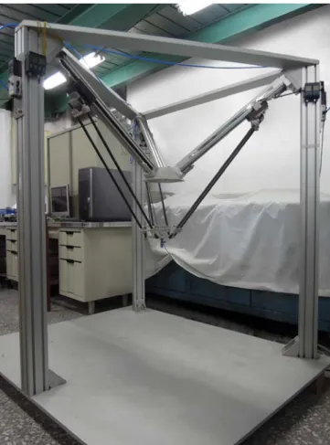
Fig. 2.3 Photograph of the three-axial pyramidal pneumatic parallel manipulator

(31)

2.2 Test Rig Layout

2.2.1 Pneumatic Servo Positioning System

The test rig layout of a pneumatic servo positioning system is shown in Fig. 2.4, which illustrates the single-axial pneumatic actuator system of the manipulator. The pneumatic actuator system comprises an air pressure source, a proportional servo valve and a pneumatic rodless cylinder. The pressure source is provided by an air compressor made by Taiwan Co Sheng, and the supplied air pressure is regulated at 6 bar. The servo valve is a 5/3-way proportional directional control valve made by Festo AG (model MPYE-5-M5) and is used to control the air flowing into the cylinder. A pneumatic rodless cylinder with 25 mm bore and 500 mm stroke (Festo model DGC-25-500) is used as the linear actuator. An optical linear encoder with 1 μm resolution is used as the position sensor and installed on the cylinder to measure the piston’s position. Two pressure sensors (Festo model SDE1) are connected to the two ports of the cylinder and used to measure the pressures of the two cylinder chambers.

Fig. 2.4 Test rig layout of the pneumatic servo positioning system

(32)

In the closed-loop system, the measured signals are fed back to a PC-based controller via the interface cards which are the data acquisition (DAQ) cards containing counters (CTR) and A/D converters. The input command voltage for the servo valve is given from the analogue output ports on the DAQ cards via the D/A converters. The control system is implemented on a Windows-based personal computer. The algorithms for the control system are created and built up in a Simulink model by Matlab software, and the Real Time Windows Target (RTWT) by Mathworks is utilized to automatically generate C codes and executable files from this Simulink model. The generated executable file runs in real time on the personal computer with 1 ms of sampling time (1 kHz sampling frequency) and realizes a real-time control system. This allows easy design and rapid testing of the control algorithms with the actual hardware.

2.2.2 Overall Manipulator System

The layout of the overall three-axial pneumatic parallel manipulator system is shown in Fig. 2.5. The pneumatic servo system of the manipulator contains three proportional servo valves of the same type and three identical pneumatic rodless cylinders. The three rodless cylinders work together as the actuators on the three axes of the manipulator sharing the same pressure source and each axis has a linear encoder which measures the piston position of each cylinder,

y ,

_A

y and

_B

y . There are total

_C six pressure sensors which are used to monitor the chamber pressures of the three cylinders, where

P and

₁

P respectively represent the upper chamber pressure and the

₂ lower chamber pressure of each axis cylinder.

u ,

_A

u and

_B

u denote the control

_C input signals for the proportional valves of axis A, B and C, respectively.

(33)

A axis B axis C axis

Fig. 2.5 Test rig layout of the overall manipulator system

In the PC-based control unit, three DAQ cards are installed and used to output the control signals and receive the input signal data from the different sensors. The control voltages of three proportional valves are calculated by the real-time control algorithm in the computer and sent to the control valves via the analogue output channels on PCI-1720U DAQ card manufactured by Advantech. The pressure data of cylinder chamber measured by the pressure sensors are recorded by Advantech PCI-1710UL multifunctional card via the analogue input channels. Finally the piston displacements

(34)

of cylinders measured by the linear encoders are counted and recorded by the counters on PCI-6601 DAQ card produced by National Instruments. Thus, the motion control of the manipulator end-effector can be achieved by simultaneously controlling the piston positions of the three cylinders with the individual pneumatic servo positioning system.

Table 2.1 summarizes the components and the specifications of the system hardware used in the three-axial pneumatic parallel manipulator system.

Table 2.1 Specifications of system hardware

Components Manufacturer Type Specifications Air Compressor Taiwan Co Sheng AU-5 Flow rate: 500 / min l

Output pressure: 6 bar Pneumatic Rodless

Cylinder Festo DGC-25-500-KF-YSR-A Piston diameter: 25 mm Stroke: 500 mm Pneumatic Proportional

Directional Control Valve

Festo MPYE-5-M5-010-B Valve function: 5/3 way Input voltage: 0 - 10 V

Pressure Sensor Festo SDE1-D10

Pressure measuring range: 0 - 10 bar Output voltage: 0 -10 V Optical Linear Encoder Jena LIA20-L301-WA Resolution: 1

μm

Data Acquisition Card

Advantech PCI-1720U 4-ch analog output with 12-bit D/A converter

Advantech PCI-1710UL

16-ch analog input with 12-bit A/D converter 16-ch digital input/output

National Instruments PCI-6601

4-ch 32-bit counter with 20 MHz maximum

source frequency

32-ch digital input/output

(35)

Chapter 3 Path Planning Algorithms for 3D Printing

3D-printing process requires the completion of four main tasks, such as Object Orientation, Support Generation, Slicing, and Path Planning. However, path planning has a remarkable impact on the overall manufacturing time and, therefore, the algorithms play a crucial role in solving this problem.

This chapter consists of three parts. The first part is to derive the path planning model. The Graph theory is introduced first, and according to the ways of linkage between each two points, some are built in double-directions directed graph and others are in single-direction directed graph. Both of them are in vector form. The second part is the path planning strategy for a layer. The modified Depth-First Search (DFS) and the modified Genetic Algorithm (GA) are proposed to generate the sub-paths and optimize the linkages of all sub-paths. The third part is the path planning strategy for layer-to-layer, based on the proposed algorithms for a layer to cascade all layers.

3.1 Path Planning Model

Before building the path planning model, the desired printing object has to be sliced equally first, and Fig. 3.1 shows an example. 3D printing is an additive manufacturing, which builds up layer by layer, and the easiest way to establish layers is to slice horizontally. The height of layers depends on the extruder of 3D printers. In order to simplify naming layers in this thesis, the bottom layer, called Layer 1, means the first layer to manufacture, and Layer 2 means the second layer to manufacture, etc.

In Fig. 3.2, it is a three-layer object which means the bottom layer is Layer 1 and the top layer is Layer 3. Besides, the number of top layer implies that how many layers the desired printing object is composed of.

(36)

Fig. 3.1 Slicing a desired printing object equally

Fig. 3.2 The definition of layers

After slicing the desired printing object, the next step is to make each layer with equal-sized rectangular mesh, according to the resolution and extruder of 3D printers. In Fig. 3.3, a layer meshes into nine small cubes.

The last step is to choose an appropriate position as a point to represent component mesh. The best position of x-y plane, the horizontal direction of slicing, is to pick the center of shape of component mesh; the ideal position of z plane, the perpendicular direction of slicing, is at the bottom surface of component mesh, because of additive manufacturing. The result is depicted in Fig. 3.4. In the end, a 3D object is converted into 2D images, which are composed of simple points.

Layer 3

Layer 2

Layer 1

(37)

(a)

(b)

Fig. 3.3 Equal-sized rectangular mesh on a layer: (a) front view (b) top view

Fig. 3.4 The position of a point (red dot) substitutes component mesh

Graph theory [49] has a wide range of applications in engineering, in biological sciences, and in numerous other areas. A graph can be used to represent almost any physical situation involving discrete objects and a relationship among them. The Königsberg Bridge Problem is perhaps the best-known example in graph theory. It was a long-standing problem until solved by Leonhard Eular in 1736, by means of a graph [50]. Eular wrote the first paper ever in graph theory and thus become the originator of

y x

z

(38)

the theory of graphs as well as of the rest of topology.

In path planning model, the component mesh is represented as points. It is helpful to use graph conveying the relationship between points on a layer and layers. In order to express the path directions of 3D printing, a directed graph G could be considered as going form vertex

v to vertex

_i

v or from

_j

v to

_j

v , which presented as a start point

_i and an end point in an overall path trajectory. For example, Fig. 3.5 shows a directed graph with five vertices (

v v v v v ) and five edges (

₁, , , ,₂ ₃ ₄ ₅

e e e e e ).

₁, , , ,₂ ₃ ₄ ₅

Fig. 3.5 A directed graph with 5 vertices and 5 edges

On a layer, each two of adjacent points should use double directions of directed graph representing two possible straight paths between vertex

v and vertex

_a

v which

_b are adjacent points and denoted

v v 

_{a b}

and

v v 

_{b a}

e

1

(39)

v v 

c d

as an edge, or a path. Owing to additive manufacturing, the overall path trajectory must start from bottom layer and end at top later; thus, using single direction of directed graph between layers shows the characteristic of 3D printing. In Fig. 3.7, there are three points

v , in Layer 1,

₁

v , in Layer 2, and

₂

v , in Layer 3, which used single-direction

₃ directed graph to link layers from bottom to top.

Both two directed graphs, the double-directions and the single-direction, are in vector form to express all possible orientations among points before path planning and also show only an overall expected path trajectory after path planning which are introduced in Section 3.2 and 3.3.

Fig. 3.6 Double-directions directed graph on a layer before path planning

Fig. 3.7 Single-direction directed graph between layers before path planning

Layer 1

(40)

3.2 Single-Layer Path Planning Strategy

The algorithms of single-layer path planning are divided into two steps. The first step is to traverse all points on a layer and establish all sub-paths, which is introduced in Section 3.2.1 based on Depth-First Search (DFS), named modified-DFS. The second step is to find a minimum cost, means shortest lengths, of linking all sub-paths on a layer, which is introduced in Section 3.2.2 based on Genetic Algorithm (GA), named modified-GA. After that, a planned path trajectory on a layer is accomplished.

3.2.1 Path Generation

Depth-First Search (DFS) is a powerful technique of systematically traversing the edges of a given graph

G

=( , )

V E

, consists of a non-empty set of V of vertices and a set E of unordered pairs of vertices of V called edges, such that every edge is traversed exactly once, and each vertex is visited at least once. This technique, also called backtracking, was first formalized and used by Hopcroft and Tarjan in 1974 [51].

But in Section 3.1, each two points on a layer are connected in double-directions directed graph indicating all possible traversing ways; nevertheless, DFS is used on directed or undirected graphs of which edges are certainly exist. Therefore, DFS is not perfectly suitable for this case and needs modifications, named modified-DFS, which means to continue the concept of traversing all vertices on a layer.

As DFS, before using the modified-DFS, the priorities of traversing directions from a vertex to another have to be determined first and are only considered in four possible directions: Right, Left, Front, and Back. Fig. 3.8 shows the priorities of four traversing directions starting from vertex v. Right is the highest priority which means if a vertex is at adjacent right of v, it must traverse this direction first; Front is the lowest

(41)

priority which means this direction is the last consideration if other adjacent vertices have traversed before or no other adjacent vertices exist near to v.

Fig. 3.8 The priorities of traversing directions (1 is the highest priority)

Owing to only four possible traversing directions, the double-directions linkages between each two points on a layer, mentioned in Section 3.1, are therefore also considered in four directions: Right, Left, Front, and Back. In other words, the diagonal double-directions linkages are impossible to happen. For instance, there are six points on a layer in Fig. 3.9(a). The linkages among these six points are only considered in four directions and shown in Fig. 3.9(b). Apparently, the linkage between

v

_2,2, denoted the position of (2, 2), and

v , denoted the position of (3, 3), does not exist.

_3,3

0 1 2 3 4

(a)

X axis

Y axis

Points

0 1 2 3 4

(b)

X axis

Y axis

Points

Double-direction linking

Fig. 3.9 The linkages between each two points based on traversing directions:

(a) 6 points (b) double-directions linking strategy

Front

Back

Right

Left v

2 3

4

1

v

_2,4 as path trajectory of Sub-path 1.

D.

Repeat the steps from step B to step C. If no points are available in the neighborhood of last selected point in Sub-path 1, the first sub-path is finished.

In Fig. 3.10(c), the selected point are

v

_2,3, denoted the position of (2, 3),

v ,

_3,3 denoted the position of (3, 3), and

v

H.

Repeat the steps from step E to step G and name new sub-path as Sub-path 3 if any of points are still available, and so on till the former selected point in step E is the start point of Sub-path 1. In Fig. 3.10(f), the last selected point is

v ; after repeating step E again and again because of no available points, the

1,2

former selected point becomes

v which is the start point of Sub-path 1.

_1,4

I.

If no points are available in the neighborhood of the start point of Sub-path 1

except been visited, modified-DFS is completed. If not, repeat the steps from step F to step H. In Fig. 3.10(f), no points are available in the neighborhood of

v except been visited; therefore, modified-DFS is completed.

_1,4

(44)

0 1 2 3 4 5 0

1 2 3 4 5

(a)

X axis

Y axis

Points

0 1 2 3 4 5

(b)

X axis

Y axis

Points Subpath 1

0 1 2 3 4 5

(c)

X axis

Y axis

Points Subpath 1

0 1 2 3 4 5

(d)

X axis

Y axis

Points Subpath 1

0 1 2 3 4 5

(e)

X axis

Y axis

Points Subpath 1 Subpath 2

0 1 2 3 4 5

(f)

X axis

Y axis

Fig. 3.10 A general example of modified-DFS

start start

end start

completed start

start

end

(45)

Fig. 3.10 is a general example in which each point has at least one point in the neighborhood of four traversing directions; however, occasionally some points are separated into un-connected groups on a layer. For instance, Fig. 3.11(a) shows a layer with eleven points selected

v , denoted the position of (1, 4), as the start. After

_1,4 applying modified-DFS, only one sub-path, Sub-path 1, is generated which starts from

v and ends at

1,4

v , denoted the position of (1, 3), shown in Fig. 3.11(b). Apparently,

_1,3 Sub-path 1 merely includes eight points and three points are left to wait for traversing.

To solve this situation, the method is adding a counter to calculate how many points have been marked in step C and step G. Because the total amount of points on a layer is given, the advantage is to make sure each point belongs in one of sub-paths. If the counter does not match up after first modified-DFS, finding a nearest point to the first start point, because modified-DFS ends when backing to the start in step I, to turn into a new start point as second modified-DFS, and so on till the counter matches the total amount of points on a layer. By continuing the case in Fig. 3.11, the nearest point to

v , the start of first modified-DFS, is

_1,4

v

_4,3, denoted the position of (4, 3), which becomes the new start point of second modified-DFS and shown in Fig. 3.12(a). After applying second modified-DFS in Fig. 3.12(b), Sub-path 2 is generated and starts from

v

4,3 and ends at

v , denoted the position of (4, 1). The counter is eleven which means

_4,1 each point has been traversed and no needs to try third modified-DFS.

Fig. 3.13 is a complete example including the exception. Fig. 3.13(a) shows a layer with forty-five point selected

v as the start. In Fig. 3.13(b), Sub-path 1, Sub-path 2

_1,8 and Sub-path 3 are generated during first modified-DFS; Sub-path 4 is established during second modified-DFS. After these, the counter is forty-five and each point has been traversed, which means the first step of single-layer path planning is finished.

(46)

0 1 2 3 4 5 0

1 2 3 4 5

(a)

X axis

Y axis

Points

0 1 2 3 4 5

(b)

X axis

Y axis

Points Subpath 1

Fig. 3.11 The exception in modified-DFS:

(a) 11 points (b) some un-traversed points after modified-DFS

0 1 2 3 4 5

(a)

X axis

Y axis

Points Subpath 1

0 1 2 3 4 5

(b)

X axis

Y axis

Fig. 3.12 Solution of the exception in modified-DFS:

(a) selecting a new start point nearest to the start point of Sub-path 1 (b) using modified-DFS again and checking the counter when completed

start start

end

counter = 11

start

end start(old)

start(new)

counter = 8

(47)

0 1 2 3 4 5 6 7 8 9 0

1 2 3 4 5 6 7 8 9

(a)

X axis

Y axis

Points

0 1 2 3 4 5 6 7 8 9

(b)

X axis

Y axis

Points Subpath 1 Subpath 2 Subpath 3 Subpath 4

Fig. 3.13 A complete example of modified-DFS including the exception:

(a) 45 points (b) 4 sub-paths after modified-DFS

3D列印之路徑規劃演算法於三軸氣壓式並聯機構機械臂之研究

國立臺灣大學工程科學及海洋工程學系 碩士論文

Department of Engineering Science and Ocean Engineering College of Engineering

National Taiwan University Master Thesis

3D 列印之路徑規劃演算法

於三軸氣壓式並聯機構機械臂之研究 The Development of Path Planning Algorithm

for 3D Printing

in a Three-Axial Pneumatic Parallel Manipulator

温志培 Chih-Pei Wen

指導教授：江茂雄 博士

Advisor: Dr.-Ing. Mao-Hsiung Chiang

中華民國 105 年 1 月

January, 2016

誌謝

中文摘要

ABSTRACT

CONTENTS

Chapter 1 Introduction ... 1

Chapter 2 System Overview ... 8

Chapter 3 Path Planning Algorithms for 3D Printing ... 15

Chapter 4 Analysis of Kinematics ... 36

Chapter 5 Controller Design ... 43

Chapter 6 Simulations and Experiments ... 50

Chapter 7 Conclusions ... 138

LIST OF FIGURES

1 i +

i + 1

i + 1

z = − 300

z = − 270

z = − 240

z = − 300

z = − 270

z = − 240

z = − 300

z = − 270

z = − 240

z = − 300

z = − 270

z = − 240

LIST OF TABLES

Chapter 1 Introduction

1.1 Background

1.2 Literature Review

1.2.1 Parallel Manipulator

al. [10]. In 2011, Chiang and Lin developed a parallel manipulator driven by three

1.2.2 Pneumatic Servo System

1.2.3 3D Printing Technology

1.3 Motivation

1.4 Outline of Thesis

Chapter 2 System Overview

2.1 Mechanism Description

Limb B Limb A

Limb C

Fixed Base

Moving Platform

z

x o y

2.2 Test Rig Layout

2.2.1 Pneumatic Servo Positioning System

2.2.2 Overall Manipulator System

y ,

y and

y . There are total

P and

P respectively represent the upper chamber pressure and the

u ,

u and

u denote the control

A axis B axis C axis

A axis B axis

C axis

u

P

P

y

u

P

P

y

國立臺灣大學工程科學及海洋工程學系碩士論文

指導教授：江茂雄博士