以物種分布模式預測台灣北部兩種攀蜥的共域區並檢視形態置換現象

國立臺灣大學生命科學院生態學與演化生物學研究所 碩士論文

Institute of Ecology and Evolutionary Biology College of Life Science

National Taiwan University Master Thesis

以物種分布模式預測台灣北部兩種攀蜥的共域區 並檢視形態置換現象

Examining the Pattern of Character Displacement of Two Sympatric Agamid Lizards in Northern Taiwan by Species

Distribution Model

陶善達 Shan-Ta Tao

指導教授：林雨德 博士 Advisor: Yu-Teh K. Lin, Ph.D.

中華民國102年6月

June, 2013

i

誌謝

這篇論文的完成首先必須感謝林雨德老師在過去這三年半之間耐心的指導，以及三位口 試委員李培芬老師、林思民老師、陳賜隆博士在口試期間給予的指教與建議，讓論文的呈現 更臻完整。

在這段期間中，有許多人的協助使得本篇研究可以順利完成。首先要感謝師大草魚實驗 室的林思民老師以及實驗室成員：阿傑、龍哥、展蔚、彥博、芳神、阿平……等人在這段期 間，除了提供詳近採樣的資訊以供參考，也讓我可以更進一步的學習有關兩爬的知識，也提 供了我進入學術研究的訓練機會；也要感謝小蛇與阿宏提供的野外資訊。台大空間生態研究 室的李培芬老師以及怡慧學姊，感謝在這段期間內教導我對於地理資訊系統的相關知識與操 作，以及資料的分析與判讀，也提供了很多分析上的想法；感謝承恩學長，在野外採樣資訊 上的提供以及陪伴，對於共域點的資訊與分析給予了不少建議；感謝欽國學長在研討會的期 間與我討論變數的分析與選擇，讓我在後續分析中不至於茫然失措。感謝動物園的陳賜隆博 士，給予我機會在動物園內進行調查，同時也告知許多非常有用的分布資料。感謝台大動物 生態研究室的威廷以及艾陵，在野外採樣上給予的大力協助；感謝已畢業的邵閔學長及徵葳 學姊提供研究上的想法；感謝淑蕙學姊、菡芝學姊、佳倩、柏翰、貝珊、允光、友志、文皓、

雨珊、丞雅、哲豪、威森、慶賀、蟲子，若沒有你們在精神上的支持與陪伴，我也無法如此 專注的完成這篇研究。感謝許許多多的好朋友提供分析與想法上的建議，以及你們實質與精 神上的支持。

感謝這片大自然賜予我進行研究的機會，在這個過程當中如有因採集過程的疏失造成傷 害的生物，在此致上歉意，所有的資訊我都會善加利用，並妥善保存。最後也要感謝我的母 親與妹妹大力支持我繼續碩士生涯，在這麼長的時間中，始終願意支持我走下去。

ii

摘要

形態置換假說：當形態相似的物種共存於同一群聚時，同一物種於共域區的族群會在一 個或多個形態上產生分化。透過形態上差異的增加，可降低對於限制性資源的種間競爭強度。

斯文豪氏攀蜥(Japalura swinhonis)與黃口攀蜥(Japalura polygonata xanthostoma)皆有分布在台 灣北部地區。這兩個同屬種有相似的外觀型值與生態習性，但在巨觀棲地上有所差異。我使 用兩物種在巨觀棲地上有所差異的變數建構各物種的分布模式，預測兩物種的潛在共域區，

並由潛在共域區的資訊選擇樣區檢視兩物種的形態置換現象。物種分布模式的結果顯示對這 兩個物種出現機率影響最大的兩項因子分別是到人為土地利用密集區的距離以及森林面積，

同時預測的結果讓我得以確認四個共域區作為後續檢視形態置換現象之用。對相同物種而 言，四個共域區中有三個發現其與鄰近的非共域區在頭部相關的外觀型值顯著的變小。分析 結果也發現對共域區內的族群而言，與咬合力有關的外觀型值在確實有發現明顯的形態置換 現象；但與最大衝刺速度較有相關的外觀型值在共域區的種間差異反而降低了。形態置換現 象可能同時受到種間競爭與天敵捕食壓力的影響，因而降低兩物種在共域區的種間差異。

關鍵字：斯文豪氏攀蜥、黃口攀蜥、棲位、物種分布模式、形態置換

iii

Abstract

Character displacement hypothesis states: when species with character similarity coexist in the same community, the population in sympatric location would displace in one or more characters.

The increased differences in character space would reduce the strength of inter-specific competition for limited resources. Both Japalura swinhonis and Japalura polygonata xanthostoma occur in northern Taiwan. The two congeners have similar morphology and ecology, yet different

macro-habitats. I applied species distribution model to identify environmental features that describe their differences in macrohabitat use, and predict the potential contact zone of the two species. Then use the latter to examine the pattern of character displacement. The results of species distribution modeling showed the distance to human-use area and total area of forest contribute the most to the distribution of the two species. The models allowed me to successfully locate four main regions of species coexistence. I found evidence for character displacement in most sympatric locations of Japalura swinhonis and Japalura polygonata xanthostoma. In four of the sympatric locations I surveyed, three of them showed significant intra-specific differences in their morphology between sympatric and allopatric locations. The head related parameters were consistently smaller for both species. While inter-specific difference of bite force related characters were greater in the sympatric than allopatric locations, characters related to sprint speed were more similar in the sympatric locations. Character displacement may be effect by inter-specific competition and predation risk in sympatric location, therefore, the characters related to sprint speed would be more similar.

Keywords: Japalura swinhonis、Japalura polygonata xanthostoma、niche、species distribution model、character displacement

iv

Contents

誌謝……….. i

摘要…….……….. ii

Abstract ……..…..………..…….. iii

Introduction……….……….……….. 1

Materials and Methods…...……….………. 5

Pilot Survey………..………... 5

Field Survey for Species Distribution Modeling………... 6

Species Distribution Modeling………... 6

Identifying Potential Contact Zone……….. 9

Field Sampling for Character Displacement Analyses………. 10

Morphometric analyses………...…11

Result…..……….………....…………..……….….15

Pilot Survey………..………... 15

Field Survey for Species Distribution Modeling………... 15

Constructing Species Distribution Models………... 15

Identifying Potential Contact Zone……….. 18

Field Sampling for Character Displacement Analyses………. 18

Morphometric analyses………...…19

Discussion……….……….………21

Species Distribution Modeling……….21

The Pattern of Character Displacement………22

Conclusion……….………....……….………27

Reference.……….……28

Table……….……33

Figure……….………71

v

Appendix..………..82

vi

Contents of Tables

Table 1. Micro-habitat conditions of male and female Japalura swinhonis or

Japalura polygonata xanthostoma……….………...33

Table 2. The proportion of vegetation type in the study area, and the number of each type sampled.……….34 Table 3. The mean (±1sd) of 11 environmental variables each in 1km*1km cells with

Js-only, Jpx-only, both species, or neither species………....35

Table 4. A comparison among different occurrence types in 11 environment variables based on one-way ANOVAs………..………....36 Table 5. Pairwise Pearson’s correlation coefficient values between pairs of 11

environmental variables………..…….…..37 Table 6. Mean and median values of model performance and the contribution and

importance of each environmental variables for the 10 best suitability models for Japalura swinhonis……….……….38 Table 7. Mean and median values of model performance and the contribution and

importance of each environmental variables for the 10 best suitability models for Japalura polygonata xanthostoma……….……….……39 Table 8. The number of lizards measured at each sampling location…...…....……40 Table 9. The number of Japalura swinhonis and Japalura polygonata xanthostoma

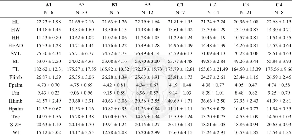
per km per survey at each sympatric location………...41 Table 10. The mean (±1sd) value of each morphometric parameter for each

treatment………42 Table 11. The mean (±1sd) value of each morphometric parameter of Japalura

swinhonis males at individual locations………43

Table 12. The mean (± 1sd) size of each morphometric parameter of Japalura

vii

swinhonis females at individual locations………...……..…..44

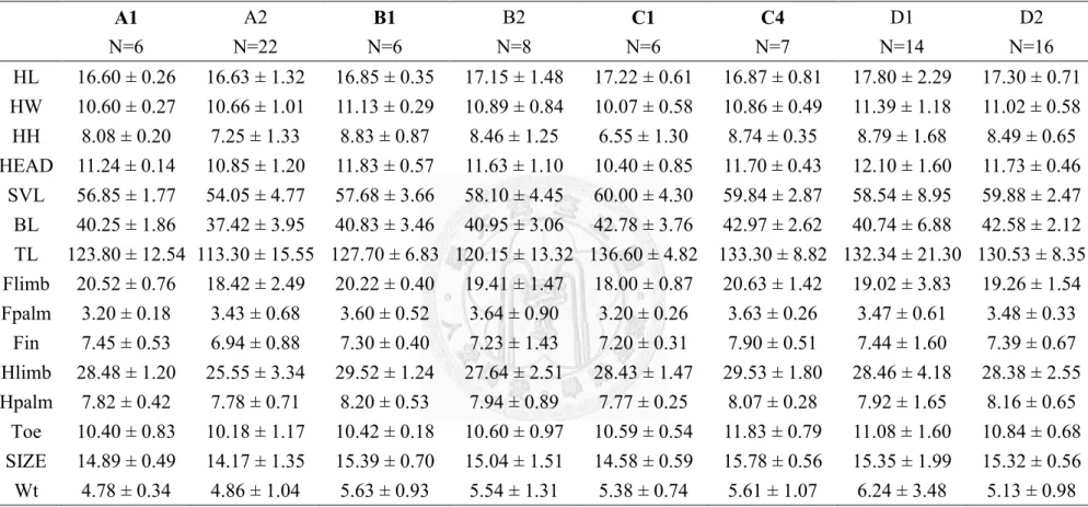
Table 13. The mean (± 1 SD) size of each morphometric parameter of Japalura polygonata xanthostoma males at individual locations………..…………45

Table 14. The mean (± 1 SD) size of each morphometric parameter of Japalura polygonata xanthostoma females at individual locations………...………46

Table 15. A comparison between sympatric and allopatric male populations in 12 standardized morphometric parameters based on one-way ANOVAs with block………47 Table 16. A comparison between sympatric and allopatric female populations in 12

standardized morphometric parameters based on one-way ANOVAs with block………48 Table 17. The comparison of two species at different locations of region A in males’

standardized morphology………49 Table 18. The comparison of two species at different locations of region A in

females’ standardized morphology.………50 Table 19. The comparison of two species at different locations of region B with

males’ standardized morphology...….………51 Table 20. The comparison of two species at different locations of region B with

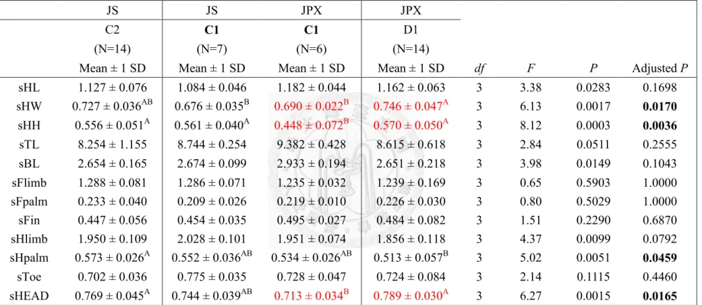
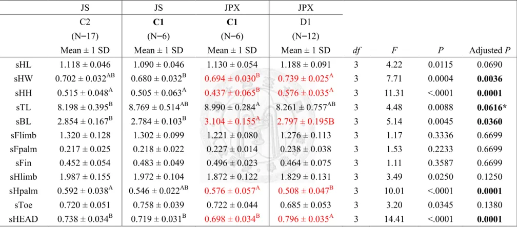
females’ standardized morphology….………52 Table 21. The comparison of two species at different locations of region C-I (C1, C2 and D1) with males’ standardized morphology..………53 Table 22. The comparison of two species at different locations of region C-I (C1, C2 and D1) with females’ standardized morphology…...………54 Table 23. The comparison of two species at different locations of region C-II (C1,

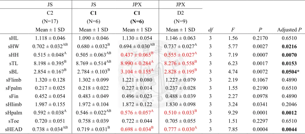
C2 and D2) with males’ standardized morphology………55

Table 24. The comparison of two species at different locations of region C-II (C1,

viii

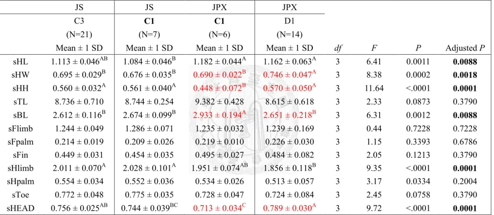
C2 and D2) with females’ standardized morphology……….…56 Table 25. The comparison of two species at different locations of region C-III (C1,

C3, D1) with males’ standardized morphology…..………57 Table 26. The comparison of two species at different locations of region C-III (C1,

C3, D1) with females’ standardized morphology...………58 Table 27. The comparison of two species at different locations of region C-IV (C1,

C3, D2) with males’ standardized morphology..………59 Table 28. The comparison of two species at different locations of region C-IV (C1,

C3, D2) with females’ standardized morphology..……….…60 Table 29. The comparison of two species at different locations of region C-V (C2,

C4, D1) with males’ standardized morphology..………61 Table 30. The comparison of two species at different locations of region C-V (C2,

C4, D1) with females’ standardized morphology..……….…62 Table 31. The comparison of two species at different locations of region C-VI (C2,

C4, D2) with males’ standardized morphology..………63 Table 32. The comparison of two species at different locations of region C-VI (C2,

C4, D2) with females’ standardized morphology..……….…64 Table 33. The comparison of two species at different locations of region C-VII (C3,

C4, D1) with males’ standardized morphology..………65 Table 34. The comparison of two species at different locations of region C-VII (C3,

C4, D1) with females’ standardized morphology..……….…66

Table 35. The comparison of two species at different locations of region C-VIII (C3,

C4, D2) with males’ standardized morphology..………67

Table 36. The comparison of two species at different locations of region C-VIII (C3,

C4, D2) with females’ standardized morphology..……….…68

Table 37. Summary of significant intra-specific difference in morphometric

ix

characters between sympatric and allopatric populations…...……...……69 Table 38. A list of morphometric parameters of males and females in different region

that showed character displacement………....……...……70

x

Contents of Figures

Figure 1. Concept map of the current study ………..…………...….71 Figure 2. Japalura occurrence in 90 surveyed cells in northern Taiwan…………...72 Figure 3. Japalura occurrence in 120 cells………....73 Figure 4. The relationship between probability of species occurrence and the

distance to human-inhabited area………....…...74 Figure 5. The relationship between probability of species occurrence and average

elevation………..75 Figure 6. The relationship between probability of species occurrence and the total

area of forest………..…....…..76 Figure 7. The relationship between probability of species occurrence and the mean

precipitation of breeding season…………...…77 Figure 8. A simplified map of occurrence probability for Japalura swinhonis in the

study area………...…….78 Figure 9. A simplified map of occurrence probability for Japalura polygonata

xanthostoma in the study area...………...…..79

Figure 10. Potential contact zones of Japalura swinhonis and Japalura polygonata xanthostoma………...……80 Figure 11. Sampling locations for examining the pattern of character displacement

of Japalura swinhonis and Japalura polygonata xanthostoma...………..81

xi

Contents of Appendices

Appendix I. Micro-habitat conditions of female and male Js or Jpx.………..82 Appendix II. A comparison among different occurrence types in 11 environment

variables based on one-way ANOVAs………...………83 Appendix III. Comparison between sympatric and allopatric populations in 12

standardized morphometric parameters……….……...84 Appendix III-1. A comparison between sympatric and allopatric male

populations- full ANOVA tables.. ….……….…. ……….…84 Appendix III-2. A comparison between sympatric and allopatric female

populations- full ANOVA tables…. …..………85

Appendix III-3. The comparison of two species at different locations of region A

with males’ standardized morphology- full ANOVA tables.. ….…. …………86

Appendix III-4. The comparison of two species at different locations of region A

with females’ standardized morphology- full ANOVA tables….…. …………87

Appendix III-5. The comparison of two species at different locations of region B

with males’ standardized morphology- full ANOVA tables.. ….…. …………88

Appendix III-6. The comparison of two species at different locations of region B

with females’ standardized morphology- full ANOVA tables….…. …………89

Appendix III-7. The comparison of two species at different locations of region

C-I with males’ standardized morphology- full ANOVA tables.. ….…. ……..90

Appendix III-8. The comparison of two species at different locations of region

C-I with females’ standardized morphology- full ANOVA tables.. …... ……..91

Appendix III-9. The comparison of two species at different locations of region

C-II with males’ standardized morphology- full ANOVA tables.. ….….……..92

Appendix III-10. The comparison of two species at different locations of region

C-II with females’ standardized morphology- full ANOVA tables.. …... …….93

xii

Appendix III-11. The comparison of two species at different locations of region

C-III with males’ standardized morphology- full ANOVA tables.. ….….…….94

Appendix III-12. The comparison of two species at different locations of region

C-III with females’ standardized morphology- full ANOVA tables.. …... ……95

Appendix III-13. The comparison of two species at different locations of region

C-IV with males’ standardized morphology- full ANOVA tables.. ….….…….96

Appendix III-14. The comparison of two species at different locations of region

C-IV with females’ standardized morphology- full ANOVA tables.. …... ……97

Appendix III-15. The comparison of two species at different locations of region

C-V with males’ standardized morphology- full ANOVA tables.. …..….…….98

Appendix III-16. The comparison of two species at different locations of region

C-V with females’ standardized morphology- full ANOVA tables.. …... .……99

Appendix III-17. The comparison of two species at different locations of region

C-VI with males’ standardized morphology- full ANOVA tables.. ….…...….100

Appendix III-18. The comparison of two species at different locations of region

C-VI with females’ standardized morphology- full ANOVA tables.. …... …..101

Appendix III-19. The comparison of two species at different locations of region

C-VII with males’ standardized morphology- full ANOVA tables.. ….….…..102

Appendix III-20. The comparison of two species at different locations of region

C-VII with females’ standardized morphology- full ANOVA tables.. …... ….103

Appendix III-21. The comparison of two species at different locations of region

C-VIII with males’ standardized morphology- full ANOVA tables.. ….…….104

Appendix III-22. The comparison of two species at different locations of region

C-VIII with females’ standardized morphology- full ANOVA tables.. …...…105

Appendix IV. Sampling effort at each sampling location.……...………..106

1

Introduction

In The Struggle for Existence, Gause (1934) stated that two species with similar

ecological requirements cannot coexist in the same community indefinitely. It was

later named ”the Principle of Competitive Exclusion” (Hardin 1960). To coexist,

species must partition sufficiently on one or more niche axes such as time, space, or

resource use, thus increase the strength of intra-specific competition relative to

inter-specific competition (Amarasekare, 2003). Sympatric species, particularly

closely related species, with similar character features may potentially face greater

competitive pressure due to the overlap in resource usage. Character displacement is a

mechanism by which competing sympatric species can enhance the segregation of

niche from each other. It is a situation when two species are allopatric, they may be

similar to each other; when they co-occur, they would “displace” one or more

characters and become dissimilar (Brown & Wilson, 1956). The characters can be a

suit of traits in morphology, behavior, physiology, or life-history. The displacements

are assumed to be genetically based. They define the evolution of character difference

that would reduce the resource use overlap and interspcific competition as “ecological

character displacement”.

The classic example of character displacement was found in Darwin’s finches.

Geospiza fortis diverged in beak size from a co-existing competitor, G. magnirostris,

2

when they experienced intensive competition for food during years of severe drought

(Grant & Grant, 2006). Losos (1994) in another classic case of character displacement

demonstrated that with the absence of ecologically similar specie, anole species

tended toward an optimal body size. In multi-species communities, competitive

interactions forced species deviate from the optimal size. Sympatric members of the

same eco-morph type became different greatly in sizes. The populations alter their

resource use in the presence of ecologically similar congeners. The study by Pfennig

& Murphy (2000) on Plains (Spea bombifrons) and Mexican (Spea multiplicata)

spadefoot toads showed that most tadpoles of former species became carnivorous

while the latter species remained mostly omnivorous in the sympatric breeding ponds.

Recently, Pfennig et al. (2006) showed that the two species could only coexist where

breeding ponds had sufficient food resources. That is, only when a habitat was

suitable for both species to coexist, would character displacement occur. In addition,

they argued that since demographic changes occur on a shorter time scale than genetic

changes, character divergence should be a plastic response initially. If the resource

remained sufficient to allow both competitors to persist, then the divergence may

become genetically canalized (Pfennig & Pfennig, 2012). My research project

examines the ecological character displacement of two sympatric agamid lizards in

northern Taiwan.

3

The two lizard species, Japlura swinhonis and Japalura polygonata xanthostoma,

inhabit low elevation area (below 1500m) in northern Taiwan. Japalura polygonata

xanthostoma (Jpx, hereafter) distributes mostly in northern Taiwan, while Japlura

swinhonis (Js, hereafter) populates the whole island (Hsiang, 1997; Ota, 1991). The

two congener (Hsiang 1997) species have similar morphology and ecology. There was

little difference between species in daily active patterns, breeding seasons, home

range sizes, diets, and perch usage (Lin & Lu, 1982; Kuo et al., 2007; Yang, 2009).

Previous studies (Lue et al., 1987; Zeng & Gao, 2004) have shown that there is often

only one species occur in surveyed locations. Js frequently appears in relatively open,

human-disturbed habitats, such as city parks or school campuses. Jpx, on the other

hand, appears mostly in mountain foothills. Despite the perceived (not formally

quantified) differences in macro-habitat use, anecdotal information suggested that the

two species co-occur at a number of locations in northern Taiwan. At such a

sympatric location, in comparison with two allopatric locations, Yang (2009) found

apparent character displacement between the two agamid lizards. That is, the

dissimilarity in morphology was greater at the sympatric than allopatric locations. It

became clear that an investigation on the pattern of character displacement at a large

spatial scale would provide insights on the distribution of and competition between

the two species.

4

As an initial step, I employed the species distribution modeling technique

(Ferrier & Guisan, 2006) to identify environmental factors that may contribute to the

distribution patterns of each species in northern Taiwan. A species distribution model

combines the presence-only or presence-absence data with environmental variables to

predict species occurrence probability over an area (Elith & Leathwick, 2009). The

idea is based on Hutchinson’s description of a species niche as an “n-dimensional

hyper-volume” (Hutchinson, 1957). I then used the species distribution models to

predict the locality of allopatry or sympatry, particularly the latter, of the two agamid

lizards. Sample locations of allopatry or sympatry were surveyed and confirmed of

their status. Finally, I sampled lizards in several regions with both allopatry or

sympatry populations to examine the pattern of character displacement. Overall, my

research aims are three folds: (1) To identify the environmental variables contribute to

the distribution of Js and Jpx; (2) To determine the locations of allopatry or sympatry

of Js and Jpx; (3) To reveal the pattern of character displacement between Js and Jpx.

Finally, I discuss the evolutionary implication of character displacement on the

co-existence of Js and Jpx. Figure 1 gives the concept map of the current study.

5

Materials and Methods

1. Pilot Survey

I conducted a pilot survey during 2009~2010 in order to have some idea about the

habitat requirements of Js and Jpx. It later helped me select meaningful environmental

factors for species distribution modeling. I visited 30 locations in northern Taiwan.

Other than noted the macro-habitat type of each location, such as urban area and

foothill, when a Js or Jpx was spotted, I measured temperature and relative humidity

in situ with a hand-held weather station. I also measured canopy coverage by taking a

vertical bottom-up picture of the canopy with a digital camera with a 35-mm lens. The

images were processed with software Image J (ver.1.44, Abramoff, Magalhaes, &

Ram, 2004) to calculate the coverage of canopy. One-way ANOVAs were applied to

compare between four sex-species categories. The inflation of p values due to tests on

multiple parameters was corrected with the Benjamini-Hochberg FDR-controlling

adjustment (a sequential Bonfferoni correction). Comparisons with significant test

results were followed by post hoc pairwise comparisons using the Scheffé’s tests. The

signicance level of all statistical tests was set at p < 0.05. I reported values as

mean±1sd. All statistical tests used in this thesis followed the same procedures unless

stated otherwise.

6

2. Field Survey for Species Distribution Modeling

The range of study area covered the Taipei City, the New Taipei City, and the

north-east corner of Taoyuan county (24° 43’ 40” ~ 25° 17’ 58” N, 121° 15’ 09” ~

122° 00̕’ 18” E). I divided the area into 2777 1-km-by-1-km grid cells (Fig. 2) that

matched the 1-km resolution of all environmental data obtained (see below). I

stratified random sampled 90 cells according to the proportions of different vegetation

types in study area (Table 2). For each sampled cells, I surveyed agamid lizard

populations along a ~500m transect. Each transect was walked in a relaxed strolling

speed, and surveyed at least twice from May to July in 2012. Because the survey of

the 90 cells yielded 21 Js-only and 41 Jpx-only cells (see Results), I also used

presence-only data from 30 non-sampled cells that came from pilot survey in

2009~2010 (see previous section) to increase sample sizes. Overall, a total of 38 and

54 cells provided information for Js and Jpx, respectively, for constructing the species

distribution models (Fig. 3 and Table 3). I did not include information from any

sympatric cells for model construction.

3. Species Distribution Modeling

I developed a species distribution model for each species using the software

7

Maxent (v.3.3.3, Phillips, et al. 2006). The software uses the maximum entropy

approach (a machine-learning algorithm) that combines presence-only data and

environmental variables to generate species distribution models (Phillips, 2004;

Cunningham et al., 2009). The maximum entropy approach performed relatively well

with small sample sizes comparing to other methods, such as GARP and Random

Forest, that also use presence-only data (Papeş & Gaubert, 2007; Hernandez et al.,

2008; Kumar & Stohlgren, 2009; Bean et al., 2012).

I chose 11 environmental variables (Table 3) that likely affect Agamid lizard

distribution to construct models. Ten of the variables (with abbreviations) were

readily available from the GIS database in the NTU Spatial Ecology Laboratory, last

updated in 2008. They included: mean altitude (DTM_MEAN); number of forest

patches (FOR_PATCH), total area of forest (FOR_AREA), mean temperature during

May-Oct. (Japalura breeding season) (T_BREEDING), accumulated monthly mean

temperature - 5℃ (5℃ is assumed the minimum temperature required for plant

growth, Kira, 1945a and b) (WARMTH), mean precipitation during May-Oct.

(P_BREEDING), direct light sky hours (DLS_HOUR), whole light sky

(WLS_HOUR), distance to 65% human land-use area (D2_H_USE), shortest distance

to Taipei City (D2_CITY), distance to the nearest road (DIS_ROAD) (Lee et al.,

1997). In addition, I calculated the distance to human-use area (D2_H_USE). It was

8

defined as the distance to the center of the nearest cell in which the proportion of

human-used area is higher than 65% (Lee et al., 1997). The parameter was different

from the distance to city (D2_CITY), which was defined as the distance to the boarder

of city. The former variable would give a better indication of the distance from one

cell to a highly developed area. I applied one-way ANOVAs to compare among cells

with Js-only, Jpx-only, both species, or neither species for each environmental

variable (Table 3 and 4). I then examined the collinearity of the remaining variables

by Pearson’s correlation coefficient. If a correlation coefficient was ≧0.60 between a

pair of two variables (Arif et al., 2007; Martínez-Freiría et al., 2008; McCormack et

al., 2010; Gormley et al., 2011; Heinänen et al., 2012; Martin et al., 2012), only one

of the variable would be selected for the species distribution model (Table 5).

All selected environmental variables were entered into Maxent software as one

CSV file. I randomly assigned 75% of the data (90 of 120 cells) as training data,

another 25% (30 cells) as testing data by bootstrapping. I chose the 10 best models out

of 30 replicates to calculate the mean and median values of testing data AUC and

omission rate as model performance indices; and to establish the 10-percentile logistic

threshold for species occurrence criteria (Hernandez et al., 2006; Phillips et al., 2006).

Generally, low omission rate (<0.1) and high AUC value (> 0.7) indicate excellent

model performance (Medley, 2010; Phillips et al., 2006). Probability of occurrence

9

for each cell was calculated from the median of all 30 replicate models in order to

reduce the effect of extreme values. Nevertheless, the qualitative results were the

same regardless of using 10 or 30 models. A map of occurrence probability was

produced for each species by using ArcGIS 9.3 (Environmental System Research

Institute, Redlands, USA).

4. Identifying Potential Contact Zones

Combining the resulting species distribution models for Js and Jpx each provided

prediction for locations of sympatry, i.e., contact zones. Locations with high

suitability for both species inferred high probability for supporting the coexistence of

Js and Jpx. I employed the Natural-Breaks classification scheme followed by an

algorithm proposed by Jenks (1967) performed in ArcGIS 9.3 to classify all cells. If

the suitability value of a cell did not reach the 10-percentile logistic threshold, it was

given a 0. Cells with suitability values higher than 10-percentile logistic threshold

were classified into three classes: 1, 2, and 3 according to their suitability values. The

classification procedure was conducted for both species separately, and a simplified

map of occurrence probability was produced for each species. The Natural-Breaks

method maximizes the difference between classes. There were 16 possible status for

each cell, from [0,0] being neither species would occur to [3,3] being both species

10

would very likely occur. To reduce the number of classes, I regrouped classes to

indicate the probability of co-occurrence: [0,0],[0,1], [1,0], [0,2], [2,0], [0,3], [3,0]

cells were grouped as N (for 0 probability); [1,1], [1,2], [2,1], [1,3], [3,1] cells were

grouped as L (for low probability); [2,2] cells remained as M (for medium

probability); [3, 2], [3, 2], [3, 3] cells were grouped as H (for high probability). This is

a more conservative approach to identify the contact zones of Js and Jpx.

5. Field Sampling for Character Displacement Analyses

After identifying contact zones, I set out to sample lizards for character

displacement analyses. I established 4 sampling regions (Fig. 10), both Regions A and

B had Js-only cells, Jpx-only cells, and Js-Jpx sympatric cells; Region C had no

Jpx-only cells, and Region D had no Js-only cells and Js-Jpx sympatric cells. Detail

information of the 4 region (Fig. 11) follows: Region A- Yinghua Ecological Park

(25° 02’ 41” N, 121° 025’ 25”E, Sympatric), Mt. Guanyin (25° 07’ 29” N, 121° 025’

29”E, Jpx-only), and Hutou Mountain Park (25° 00’ 30” N, 121° 19’ 35”E, Js-only);

Region B- Shuiguan Rd. Hiking Trail (25° 07’ 49” N, 121° 32’ 7”E, Sympatric),

Chinese Culture University (25° 08’ 05” N, 121° 032’ 18”E, Jpx-only), and

Junjianyan Hiking Trail (25° 07’ 35” N, 121° 31’ 00”E, Js-only); Region C- Taipei

City Zoo (24° 59’ 44” N, 121° 35’ 10”E, Sympatric), Chihnan Temple Hiking Trail

11

(24° 59’ 00” N, 121° 34’ 59”E, Sympatric), Xianjiyan Hiking Trail (24° 59’ 12” N,

121° 33’ 12”E, Js-only); and Mt. Fuzhou Hiking Trail (25° 01’ 03” N, 121° 33’ 10”E,

Js-only); Region D- Mt. Jinmian Hiking Trail (25° 05’ 08” N, 121° 34’ 48”E,

Jpx-only), and Neigou River Hiking Trail (25° 05’ 12” N, 121° 37’ 21”E, Jpx-only).

During survey, the total number of lizards I observed, the length of survey trail,

and the time-spent during each survey was recorded. I standardized the number of

individuals with the length of sampling trail. I arbitrarily determined 3 is the

minimum number of adult individuals for a population to be viable. For example,

Junjianyan Hiking Trail had 1,Jpx recorded. This location was considered Js-only

locations. Lizards were captured by hand or noose. For Js, male and female

individuals with snout-ventral length (SVL, hereafter) longer than 54- and 48-mm,

respectively, were considered adult; for Jpx, male and female had SVL longer than

45- and 44-mm, respectively, were considered adults (Yang, 2009). Of each captured

lizard, I recorded species, sex, conditions (parasite and injury), and morphometric

parameters (see Morphometric Analyses). Only information for adults entered

subsequent analyses.

6. Morphometric analyses

I measured body weight and the following morphological variables of lizards:

12

head length (HL, measured from quadrate to the tip of snout), head width (HW, the

distance between jaw joints on each sides), head height (HH, measured from lower

dentary to the parietal), snout-ventral length (SVL, measured from the cloacal

opening to the tip of snout), tail length (TL, measured from cloacal opening to the tip

of tail), right forelimb length (Flimb, measured from the upper arm joint to wrist),

right forelimb palm length (Fpalm, measured from wrist to the base of longest toe),

length of the longest toe of right forelimb (Fin, measured from toe base to tip, claws

were not included), right hindlimb length (Hlimb, measured from the upper leg joint

to ankle), right hindlimb palm length (Hpalm, measured from wrist to the base of

longest toe), length of the longest toe of right hindlimb (Toe, measured from toe base

to tip, claws were not included). Body length (BL) was obtained from the differences

between SVL and HL. Weight was measured to the nearest 0.1 g with a spring scale

(Pescola). Tail length was measured to the nearest 1 mm with a measuring tape. All

other morphological variables were measured to the nearest 0.1mm by a metal caliper.

I checked if outliers occurred. An individual was defined as an outlier if its two or

more morphometric parameters showed up as outliers in the outlier tests. I removed

these individuals from subsequent analyses.

I generated shape variables based on Mosimann’s method (Mosimann, 1970) as

described in Butler and Losos (2002) for each individual. I first calculated the general

13

size and head size. The general size (SIZE) was defined as the geometric mean of HL,

HW, HH, BL, TL, Flimb, Fpalm, Fin, Hlimb, Hpalm, and Toe, and head size (HEAD)

as the geometric mean of HL, HW, and HH. Each morphological variable was then

standardized by dividing it by SIZE. The standardized morphometric parameters

include: sHL, sHW, sHH, sBL, sTL, sFlimb, sFpalm, sFin, sHlimb, sHpalm, sToe,

sHEAD. Standardized parameters enter the following ANOVA analyses. Normality

tests were conducted prior ANOVA. The parameters failed the normality assumption

were nature-log transformed.

To compare the morphological characteristics between individuals in allopatric

and sympatric locations, I first applied a one-way ANOVA with block, followed by

Scheffé’s post hoc pairwise comparisons to examine the overall pattern. Region

served as blocks in this analysis. Because sexual dimorphism occurs in both Js and

Jpx (Kuo et al., 2009), males and females were analyzed separately. To examine

details within regions, I then applied a one-way ANOVA for each region, followed by

Scheffé’s post hoc pairwise comparisons. Since both Jpx-only locations of region D

were the closest allopatric sites of Japalura polygonata xanthostoma to the sympatric

locations in Region C, both regions were combined to examine the morphological

differences between sympatric and allopatric locations. Based on character

displacement hypothesis, characters with intra-specific difference in sympatric

14

location may indicate sympatric species diverged on these characters. The characters

with significant intra-specific difference between sympatric and allopatric location

were noted. For region C and D, each sympatric location compared with 4 sets of

allopatric location (two Js-only, C2 and C3 with two Jpx-only, D1 and D2),

respectively. The characters with significant intra-specific difference were noted only

when they showed statistical significance for over 3 among 4 sets of comparison. I

calculate the inter-specific difference of noted characters in sympatric and allopatric

location. I then applied a one-tailed Wilcoxon-Mann-Whitney test (a Wilcoxon

two-sample test) for comparison.

15 Results

1. Pilot Survey

The pilot survey showed there was no significant difference between Js and Jpx

in micro-habitat temperature (One-way ANOVA, F3, 234?=2.43, p=0.13) and canopy

coverage (F3, 234=0.76, p=0.52). However, the relative humidity was lower for Js than

Jpx micro-habitats (species effect, F3, 234=22.45, p = 0.0001, Table 1).

2. Field Survey for Species Distribution Modeling

Among the 90 cells I surveyed, there were 21 Js-only, 41 Jpx-only, 7 both species,

and 21 neither species cells (Fig. 2). After combining presence-only data from 30

non-sampled cells that came from the pilot survey, I had a total of 38 Js-only, 54

Jpx-only, 7 both species, and 21 neither species cells (Fig. 3). The information in the

Js-only and Jpx-only cells each was used for constructing the species distribution models for Js and Jpx, respectively.

3. Constructing Species Distribution Models

Individually, each of the 11 environmental variables had significant effects on

Japalura occurrence (Table 3). I selected 5 variables, including FOR_PATCH,

16

FOR_AREA, T_BREEDING, P_BREEDING, DLS_HOUR, according to the

Pearson’s correlation coefficient r ≧0.60 criterion. I also included DTM_MEAN and

P_BREEDING because the former variable was the only topological variable, and

P_BREEDING was related to relative humidity of microhabitat, which was a

significant micro-habitat variable (Table 1). Overall, 7 variables were selected (Table

5).

Model performance indices indicated that the mean and median of testing data

AUC for Js (Table 6) and Jpx (Table 7) were all higher than 0.8. None of the testing

data omission rates were higher than 0.0833 (Table 6 and 7). Together, they indicated

the resulting species distribution models would be accurate in predicting species

occurrence (Swets, 1988). The map of species distribution based on the models was

shown in Figure 8 for Js, and Figure 9 for Jpx. High values indicated high suitability,

thus high probability of occurrence. Results derived from mean or median values both

indicated that the environmental variables that affected Js occurrence were

FOR_AREA and D2_H_USE (Table 6). Total area of forest (FOR_AREA)

contributed ~70% in predicting Js occurrence, the greater the forest area, the lower

the probability of occurrence. Whereas, distance to 65% human land-use area

(D2_H_USE) contributed ~15%, the closer the distance to human-inhabit area, the

higher probability of occurrence. On the other hand, results derived from either mean

17

or median values indicated that 4 environmental variables affected Jpx occurrence:

FOR_AREA (~32% contribution), the greater the forest area, the higher the

probability of occurrence; D2_H_USE (~30% contribution), the closer the distance to

human-inhabit area, the higher probability of occurrence; P_BREEDING (~12%

contribution), the higher in breeding season precipitation, the higher probability of

occurrence, and DTM_MEAN (~10% contribution), the lower in elevation, the higher

probability of occurrence (Table 7). Overall, both species tend to occur in areas close

to human inhabitation. Yet, Js has stronger affiliation with human inhabitation than

Jpx does (Fig. 4). Both species tend to occur at low elevation. Yet, Js (0~200 m)

occurs at lower elevation than Jpx (100~400 m) does (Fig. 5). While microhabitat

analyses did not showed difference in preference for canopy coverage (Table 1),

species distribution modeling indicated Js prefers areas with low forest coverage, and

Js areas with high forest coverage (Fig. 6). It is likely that relative humidity that

associated with precipitation (Fig. 7) and forest coverage makes the difference.

During breeding season, Js occurs in areas with ~60% relative humidity, Jpx in areas

with ~70% humidity (Table 1). Js occurs in areas with mean breeding season

precipitation < 300mm (272.36 ± 44.19mm, Table 3), Jpx in areas with mean

breeding season precipitation > 250mm (315.01 ± 55.45mm, Table 3).

18 4. Identifying Potential Contact Zone

The median of 10 percentile logistic threshold calculated from the 10 best models

for Js and Jpx were 0.3247 and 0.2963, respectively. The probability of species

occurrence in a cell that did not reach those thresholds was given a 0 value. A total of

2647 cells were given 0. For Js, the ranges of percentiles for class 1, 2, & 3 were

0.3248~0.4384 (246 cells), 0.4384~0.5752 (198 cells), 0.5752~0.8112 (134 cells),

respectively; for Jpx, the ranges were 0.2964~0.4200 (429 cells), 0.4200~0.5644 (314

cells), 0.5644~0.8303 (209 cells), respectively. After applying the Natural-Break

method, I produced a simplified map of occurrence probability for each species (Fig.

8 and 9). Several potential contact zones of Js and Jpx were identified (Fig. 12). A

total of 130 cells had the potential of Js and Jpx co-occurrence. Among them, 12 cells

had high, 10 medium, and 108 low probabilities. I had survey information for all the

130 cells, and observed Js-Jpx co-occurrence (at least 3 adult individuals of each

species) in only 4 cells. However, I visited the 22 cells that had medium or high

probabilities. Only 3 cells I found indeed Js and Jpx co-occurrence. However, in 4 of

the other 19 cells, I found Js and Jpx co-occurrence in adjacent cells.

5. Field Sampling for Character Displacement Analyses

The number of lizards at each sampling location varied considerably (Table 8).

19

The number of Js and Jpx per km per survey at each sympatric location is given in

Table 9. Taipei City Zoo had very high density of Js, and Jpx had dwindled from

historic record (Kuo et al., 2007; Yang, 2009). Nevertheless, the colonization,

expansion, or extinction of Js and Jpx populations are an on-going dynamics. For

example, I recently (summer 2012) discovered the appearance of Js in Mt. Jinmian

Hiking Trail.

6. Morphometric analyses

I found several outlier individuals (Table 8). After removing outliers, the mean

(±1sd) value of each morphometric parameter of Js and Jpx males and females at

individual locations are given in Table 10~14. All regions combined, character

displacement was found in sHlimb (one-way ANOVA with block, treatment effect, F3,

180=72.82, P = 0.0024) for males (Table 15) but none for females (Table 16). There was no block (region) effect. Examining character displacement in different regions, I

found no evidence of character displacement (significant difference in a

morphometric character between sympatric and allopatric populations of a species) in

region B (Table 19 & 20). For region A, character displacement were found only in

female (Table 17 & 18). Female of Jpx showed significant smaller head height (sHH,

F3, 35=6.73, P = 0.0088), head size (sHEAD, F3, 35=123.43, P = 0.0001) and longer

20

length of hind-limb (sHlimb, F3, 35=14.26, P = 0.0001) (Table 18). For region C,

Taipei Zoo (C1) showed similar trend of in 4 sets of comparison, C-I~IV (Table

21~28). Male of Jpx had significant smaller head height (Table 21, 23, 25 and 27) and

head size (Table 21, 25 and 27); female of Jpx had significant smaller head height,

head size and longer body length and length of hind-palm (Table 22, 24, 26 and 28).

Chihnan Temple Hiking Trail (C4) also showed similar trend of in 4 sets of

comparison, C-V~VIII (Table 29~36). Female of Js had significant smaller head

height width (Table 30, 32, 34 and 36). Table 37 gives the summary of the evidence

of character displacement.

For those morphometric characters with significant intra-specific difference

between sympatric and allopatric location (Table38), the inter-specific differences

were not statistically greater in sympatric location in males (Z = 1.2259, P = 0.1101)

nor in females (Z = 0.7044, P = 0.2406).

21 Discussion

1. Species Distribution Modeling

My model showed high performance (AUC between 0.8~0.9) with relatively low

omission rate (< 0.1). The most contributed variables for the distribution of Js and Jpx

is the distance to human-inhabited area and the total forest area. In addition, mean

altitude and precipitation of breeding season also contribute to the distribution of Jpx.

The results showed these variables are useful in predicting the occurrence of these

two species, respectively. Js and Jpx are both arboreal species, the coverage of forest

is important to their occurrence. In general, Js showed higher probability closing to

human-inhabited area and lower forest coverage, while Jpx showed mostly in the

opposite. There is a rising probability of occurrence with relatively low forest

coverage of Jpx. One possible reason is that there are several cells were actually very

close to human-inhabited area. With 1-km resolution, the cells of mountain area

which are close to human-inhabited area may affect the prediction of Jpx occurrence.

The result of potential contact zone anticipation showed that among 22 cells with

medium to high probability of co-occurrence of Js and Jpx, only 7 were sympatric

distributed either at the exact cell or the adjacent cell. The target species may occur in

a relatively unsuitable habitat if the immigration from source population is large

22

enough (Holt, 1985; Pulliam & Brent, 1991). At the community level, these “sink”

habitats may contribute majority of species co-occurring area (Pulliam, 2000). The

result still provides me useful information of possible sympatric localities. It also

provide informations about the possible grouping for examining the character

displacement.

2. The Pattern of Character Displacement

Ecological character displacement was not consistently found in all sympatric

location I had surveyed. The population abundance of both species in sympatric

location may provide some insight. I did not find any intra-specific differences in

Shuiguan Rd. Hiking Trail (B1), which showed the lowest abundance of Js and Jpx.

Taipei Zoo (C1) showed the highest abundance of both species, which present most

significant pattern of character displacement. Previous studies showed the resource of

sympatric location must be limited so the strength of inter-specific competition would

force coexisting species to diverge in their characters (Grant, 1972; Dayan &

Simberloff, 2005). Location with low abundance of coexisting species may not reflect

the limitation of resources. Relative abundance of coexisting species may also

indicate possible mechanisms of species coexistence with character displacement.

Slatkin hypothesized two possible mechanisms: (1) for equally abundant species,

23

there are some differences in limiting resource. With small or even unmeasurable

differences can lead to significant displacements; (2) for one species more abundant

than another, there are no differences in their resource utility niche (Slatkin, 1980).

Previous study showed relatively equal abundant of Js and Jpx in Taipei Zoo (Kuo et

al., 2007). Pilot survey also suggested there is almost no difference in the

micro-habitat of Js and Jpx. Based on the information I had, former mechanisms

could be a more plausible explaination to the coexistence of Js and Jpx.

Ecological character displacement was found mostly in Jpx of Taipei Zoo.

Previous studies showed the demographic processes can account for the differences I

observed (MacArthur et al., 1967; May & MacArthur, 1972; Slatkin, 1980). Based on

the historical trend observed from previous studies (Kuo et al., 2007; Yang, 2009), the

population of Japalura swinhonis had increased during the past few years. The pattern

of morphological difference may be disturbed by the immigrant from allopatric

population.

The morphometric parameters with intra-specific difference were mostly about

head. This is the only consistent pattern among all sympatric populations (except

region B). There are several studies indicate that the head size has negative effect on

the sprint speed of lizards (Vanhooydonck & Van Damme, 1999; Peterson & Husak,

2006; Yang, 2009). Greater head size and head height may also indicate better bite

24

force (Herrel et al., 2006; Yang, 2009). For all sets comparisons of Taipei Zoo, I

found body length and length of hind-palm are consistently greater in sympatric

location. Previous studies showed that the characters of hind limb could affect the

sprint speed of lizards (Losos & Sinervo, 1989; Losos, 1990; Garland & Losos, 1994;

Van Damme et al., 1998). Body length could also affect on sprint speed (Beuttell &

Losos 1999; Losos 1990).

Despite there are pseudo replicates in my statistical analyses, the inter-specific

morphological difference is not greater in sympatric location for every character. The

inter-specific difference of head height in both sexes of Taipei Zoo (C1) and head

width in females of Chihnan Temple Hiking Trail(C4) is greater. However, the

inter-specific difference of head size in both sexes of Taipei Zoo (C1) is smaller.

Competition is not the only force could generate similar patterns of character

divergence (Taper & Case, 1992; Schluter, 2000). There are studies suggest that

predation could enhance the character divergence (Chiba, 1999; Rundle et al., 2003)

or alter the competitive interactions (Chase et al., 2002) of coexisting species. My

results suggest the character about maneuverability (e.g., length of hind-palm, head

size) of both species became similar when they coexist. The character which affect

bite force diverged in sympatric location. Based on previous morphological and

ecological studies, Losos defined all the anole lizards into different eco-morph types

25

(Losos, 2009). The characters of Js and Jpx were both similar to Trunk-ground or

Trunk-crown type. The sympatric locations are mostly relative open forest and close

to the mountain area. The occurrence of competitor with similar eco-morph type, the

pressure of predation on Js and Jpx may be more intense in the sympatric location,

especially from birds. Two species coexist with similar and enough species abundance,

the divergence cause by inter-specific competition could be enhanced by predation.

The apparent character displacement between Js and Jpx could be observed. Once the

strength of competition decreased, predation may force Js and Jpx tend to optimize

their maneuverability. Several studies showed reproduction could severely affect

locomotor performance of females (Seigel et al., 1987; Cooper, et al., 1990; Miles et

al., 2000) which may explain why most character differences were found in females

in my research.

Previous researches formalized six criteria for to ascertain the occurrence of

ecological character displacement: (1) the pattern of differences could not occur by

chance; (2) phenotypic differences should be genetic based; (3) the differences should

result from evolutionary shifting; (4)Morphological differences should related to

differences in resource use; (5) sympatric and allopatric locations should not differ

greatly in environmental features that would affect the phenotype; (6) there must be

independent evidence for competition (Schluter & McPhail, 1992; Losos, 2000;

26

Dayan & Simberloff, 2005). For the first criteria, I found consistent pattern of the

parameters about head were smaller in three of four sympatric locations. The pattern

of differences did not occur by chance. I did not examine second criteria in this

research. The genetic based of phenotypic traits is often difficult to prove (Dayan &

Simberloff, 2005). For the third criteria, when I examined the pattern of

morphological difference in Taipei Zoo (C1) and Chihnan Temple Hiking Trail(C4),

I set up four groups of compariosn for each sympatric location (C1: C-I~IV and C4:

C-V~VIII). The differences were consistently found in all sets of comparison for

every sympatric location, respectively. The differences I found should result from

evolutionary shifting. The fourth criteria had already been examined in previous study

(Yang, 2009). There are almost no differences were found between the macro- and

micro-habitat of Js and Jpx. The independent evidence for competition was already

confirmed in previous observations (Kuo et al., 2007; Yang, 2009).

27 Conclusion

My research demonstrates the usefulness of species distribution modeling in

species with ecological similarity. The results of modeling provide very useful

information about the potential sympatric locations of Js and Jpx. Among four

sympatric locations I surveyed, Taipei Zoo showed the most apparent character

displacement between Js and Jpx. Most morphological differences were found in

female of Jpx. The morphometric parameters about head are consistently smaller in

sympatric location. Smaller head indicate better sprint speed of lizards. Although I did

not examine whether the differences in morphology were genetic based, I do find

character displacement in the sympatric location of Js and Jpx. Competition and

predation could generate similar pattern of character divergence. Both of them were

frequency-dependent ecological process. Further research should consider the relative

abundance of coexisting species and the effect on competition and predation risk in

sympatric location.

28 References

Abramoff, M. D., Magalhaes, P. J., & Ram, S. J. (2004). Image Processing with Image J. Biophotonics International, 11(7), 36-42.

Amarasekare, P. (2003). Competitive coexistence in spatially structured environments:

a synthesis. Ecology Letters, 6(12), 1109-1122.

Arif, S., Adams, D. C., & Wicknick, J. A. (2007). Bioclimatic modelling, morphology, and behaviour reveal alternative mechanisms regulating the distributions of two parapatric salamander species. Evolutionary Ecology Research, 9, 843-854.

Bean, W. T., Stafford, R., & Brashares, J. S. (2012). The effects of small sample size and sample bias on threshold selection and accuracy assessment of species distribution models. Ecography, 35(3), 250-258.

Beuttell, K. & Losos, J. B. (1999). Ecological morphology of Caribbean anoles.

Herpetological Monographs, 13, 1-28.

Brown, W. L., & Wilson, E. O. (1956). Character Displacement. Systematic Zoology, 5(2), 49-64.

Butler, M. A., & Losos, J. B. (2002). Multivariate sexual dimorphism sexual selection and adaptation in Greater Antillean Anolis lizards. Ecology, 72(4), 541-559.

Chase, J. M., Abrams, P. A., Grover, J. P., Diehl, S., Chesson, P., Holt, R. D., Richards, S. A., Nisbet, R. M., & Case, T. J. (2002). The interaction between predation and competition: A review and synthesis. Ecology Letters 5:302-315 Chiba, S. (1999). Character displacement, frequency-dependent selection, and

divergence of shell colour in land snails Mandarina (Plumonata). Biological Journal of the Linnean Society, 66, 465-479.

Cooper ., W. E., Vitt, L. J., Hedges, R., & Huey, R. B. (1990). Locomotor impairment and defense in gravid lizards (Eumeces laticeps): behavioral shift in activity may offset costs of reproduction in an active forager Behavioral Ecology and Sociobiology, 27, 153-157.

Cunningham, H.R., Rissler, L. J., & Apodaca, J. J. (2009). Competition at the range boundary in the slimy salamander using reciprocal transplants for studies on the role of biotic interactions in spatial distributions. Journal of Animal Ecology, 78, 52-62.

Dayan, T., & Simberloff, D. (2005). Ecological and community-wide character displacement: the next generation. Ecology Letters, 8(8), 875-894.

Elith, J., & Leathwick, J. R. (2009). Species Distribution Models: Ecological Explanation and Prediction Across Space and Time. Annual Review of

29

Ecology, Evolution, and Systematics, 40(1), 677-697.

Ferrier, S., & Guisan, A. (2006). Spatial modelling of biodiversity at the community level. Journal of Applied Ecology, 43(3), 393-404.

Garland, T., & Losos, J. B. (1994). Ecological morphology of locomotor performance in Squamate reptiles. In P. C. Wainwright & S. M. Reilly (Eds.), Ecological Morphology: Integrative Organismal Biology (pp. 240-302): University of Chicago

Gause, G. F. (1934). The Struggle for Existence-A Classic in Mathematical Biology and Ecology.

Gormley, A. M., Forsyth, D. M., Griffioen, P., Lindeman, M., Ramsey, D. S., Scroggie, M. P., & Woodford, L. (2011). Using presence-only and

presence-absence data to estimate the current and potential distributions of established invasive species. Journal of Applied Ecology, 48(1), 25-34.

Grant, P. R. (1972). Convergent and divergent character displacement. Biological Journal of the Linnean Society, 4, 39-68.

Grant, P. R., & Grant, B. R. (2006). Evolution of character displacement in Darwin's finches. Science, 313(5784), 224-226.

Hardin, G. (1960). The Competitive Exclusion Principle. Science, 131(3409), 1292-1297.

Heinänen, S., Erola, J., & Numers, M. (2012). High resolution species distribution models of two nesting water bird species: a study of transferability and predictive performance. Landscape Ecology, 27(4), 545-555.

Hernandez, P. A., Franke, I., Herzog, S. K., Pacheco, V., Paniagua, L., Quintana, H.

L., Young, B. E. (2008). Predicting species distributions in poorly-studied landscapes. Biodiversity and Conservation, 17(6), 1353-1366.

Hernandez, P. A., Graham, C. H., Master, L. L., & Albert, D. L. (2006). The effect of sample size and species characteristics on performance of different species distribution modeling methods. Ecography, 29(5), 773-785.

Herrel, A., Joachim, R., Vanhooydonck, B., & Irschick, D. J. (2006). Ecological consequences of ontogenetic changes in head shape and bite performance in Jamaican lizard Anolis lineatopus. Biological Journal of the Linnean Society, 89, 443-454.

Holt, R. D. (1985). Population dynamics in two-patch environments: some anomalous consquences of an optimal habitat distribution. Theoretical Population

Biology, 28(2), 181-208.

Hsiang, G. S. (1997). Phylogenetic Relationships and Biogeography in the Genus Japalura of Taiwan Base on the Variation of mtDNA Sequences. (M.D.), National Sun Yat-sen University, R.O.C. (in Chinese)

30

Hutchinson, G. E. (1957). Concluding Remarks. Paper presented at the Cold Spring Harbor Laboratory Symposium on Quantitative Biology.

Jenks, G. F. (1967). The Data Model Concept in Statistical Mapping. Cartography and Geographic Information Science, 7, 186-190.

Kira,T., 1945a, New climatic zonation in eastern Asia as a basis of agricultural geography. Kyoto Imperial University, 24p, 1945a. (in Japanese) Kira,T., 1945b. New Climatic zonation in southeastern Asia. Kyoto Imperial

University, 24p, 1945b. (in Japanese)

Kumar, S., & Stohlgren, T.J. (2009). Maxent modeling for predicting suitable habitat for threatened and endangered tree Canacomyrica monticola in New

Caledonia. Journal of Ecology and Natural Environment, 1(4), 94-98.

Kuo, C.-Y., Lin, Y.-S., & Lin, Y. K. (2007). Resource Use and Morphology of Two Sympatric Japalura Lizards (Iguania: Agamidae). Journal of Herpetology, 41(4), 713-723.

Kuo, C.-Y., Lin, Y.-T., & Lin, Y.-S. (2009). Sexual Size and Shape Dimorphism in an Agamid Lizard, Japalura swinhonis (Squamata: Lacertilia: Agamidae).

Zoological Studies, 48(3), 351-361.

Lee, P. F., Liao, C. Y., Lee, Y. C., Pan, Y. H., Fu, W. H., & Chen, H. W. (1997). An Ecological and Environmental GIS database for Taiwan. Taipei. (in Chinese) Lin, J.-Y., & Lu, K.-H.. (1982). Populaiton Ecology of the Lizard Japalura swinhonis

formosensis (Sauria: Agamidae) in Taiwan. Copeia, 1982(2), 425-434.

Losos, J. B. (1990). The Evolution of Form and Function Morphology and Locomotor Performance in West Indian Anolis Lizards. Evolution, 44(5), 1189-1203.

Losos, J. B. (1994). Integrative approaches to evolutionary ecology Anolis lizards as model systems. Annual Review of Ecology and Systematics, 25, 467-493.

Losos, J. B. (2000). Ecological character displacement and the study of adaptation.

Proceedings of the National Academy of Sciences, 97(11), 5693-5695.

Losos, J. B. (2009). Lizards in an Evolutionary Tree: Ecology and Adaptive Radiation of Anoles. University of California Press, Berkeley, USA

Losos, J. B., & Sinervo, B. (1989). The Effects of Morphology and Perch Diameter on Sprint Performance of Anolis Lizards. Journal of Experimental Biology, 145, 23-30.

Lue, K.-Y., Ye, G.-Q., Chen, S.-H., Lin, Z.-Y., & Chen, S.-L. (1987). Herpetological and amphibian survey report of the Yangminshan national park. Taipei:

Yangminshan National Park, Construction and Planning Agency Ministry of the Interior. (in Chinese)

MacArthur, R. H., & Levins, R. (1967). The Limiting Similarity Convergence, and Divergence of Coexisting Species. The American Naturalist, 101(921),

31 377-385.

Martínez-Freiría, F., Sillero, N., Lizana, M., & Brito, J. C. (2008). GIS-based niche models identify environmental correlates sustaining a contact zone between three species of European vipers. Diversity and Distributions, 14(3), 452-461.

Martin, J., Revilla, E., Quenette, P.-Y., Naves, J., Allainé, D., & Swenson, J. E.

(2012). Brown bear species distribution in the Pyrenees: transferability across sites and linking scales to make the most of scarce data. Journal of Applied Ecology, 49(3), 621-631.

May, R. M., & MacArthur, R. H. (1972). Niche overlap as a function of

environmental variability. Proceedings of the National Academy of Sciences, 65(5), 1109-1113.

McCormack, J. E., Zellmer, A. J., & Knowles, L. L. (2010). Does niche divergence accompany allopatric divergence in Aphelocoma jays as predicted under ecological speciation? Insights from tests with niche models. Evolution, 64(5), 1231-1244.

Medley, K. A. (2010). Niche shifts during the global invasion of the Asian tiger mosquito, Aedes albopictus Skuse (Culicidae), revealed by reciprocal distribution models. Global Ecology and Biogeography, 19(1), 122-133.

Miles, D. B., Sinervo, B., & Frankino, W. A. (2000). Reproductive burden, locomotor performance and the cost of reproduction in free ranging lizards. Evolution, 54(4), 1386-1395.

Mosimann, J. E. (1970). Size Allometry: Size and Shape Variables with

Characterizations of the Lognormal and Generalized Gamma Distributions.

Journal of the American Statistical Association, 65(330), 930-945.

Ota, Hidetoshi. (1991b). Taxonomic Redefinition of Japalura swinhonis Günther (Agamidae: Squamata), with a Description of a New Subspecies of J.

polygonata from Taiwan. Herpetologica, 47(3), 280-294.

Papeş, M., & Gaubert, P. (2007). Modelling ecological niches from low numbers of occurrences: assessment of the conservation status of poorly known viverrids (Mammalia, Carnivora) across two continents. Diversity and Distributions, 13(6), 890-902.

Peterson, C. C., & Husak, J. F. (2006). Locomotor Performance and Sexual Selection:

Individual Variation in Sprint Speed of Collared Lizards Copeia, 2006(2), 216-224.

Pfennig, D. W., & Pfennig, K. S. (2012). Development and evolution of character displacement. Annals of the New York Academy of Sciences, 1256, 89-107.

Pfennig, D. W., & Murphy, P. J. (2000). Character Displacement in Polyphenic Tadpoles. Evolution, 54(5), 1738-1749.