5G系統中以SDN為基礎之雲端無線存取網路資源管理

科技部補助專題研究計畫成果報告

期末報告

5G系統中以SDN為基礎之雲端無線存取網路資源管理

中　華　民　國　108　年　09　月　30　日

中 文 摘 要 ： 隨著行動裝置的普及與物聯網之快速發展，網路存取的使用量大增 ，第五代行動通訊系統便以處理大量服務需求與兼容異質網路環境 為目標，針對彈性的架構與動態的資源分配技術廣泛地討論。例如 雲端無線存取網路將傳統基地台的基頻單元佈建在雲端，使基地台 間可共享運算資源，以達到最佳化分配。而軟體定義網路則是透過 網路管理架構的軟體化與控制模組的中心化，動態且彈性地即時管 理網路服務。 在此種集中管理的網路架構下，現有的聯結管理機制並無法受益於 此。此外，當裝置數量爆炸性成長，但無線資源仍相當有限的狀況 時，在單一基地台底下，大量的聯結建立請求將導致嚴重的碰撞問 題，降低資料傳輸的成功率，造成不必要的電力浪費。在多個基地 台間，則需更全面性的負載平衡演算法，計算出最佳的聯結關係 ，提升整體的傳輸量。因此，在採用雲端無存取網路和軟體定義網 路的5G架構下，如何更有效率地控制與分配裝置與基地台之聯結 ，並處理大量的請求，需要進一步的研究探討。 本研究針對裝置數量超越基地台所能負荷的物理限制情境下，提出 將裝置分組的核心想法，以組為單位設計聯結機制，並延遲部分請 求，來提升整體網路的效率。在單一基地台底下，針對不移動的機 器間通訊，將裝置依地域分組，並由群組組長協調組內的請求排序 ，來減緩基地台的隨機存取碰撞。在多基地台間，則針對使用者攜 帶的移動裝置，透過集中的網路管理架構來取得更全面的資訊以達 到負載平衡，在群組移動後，計算出各個基地台最佳的覆蓋範圍 ，以提升吞吐量。 針對上述碰撞與負載平衡，論文中透過數學模型分析與模擬實驗來 觀察成效，結果顯示在資源供不應求的狀況下，本論文提出之機制 皆可透過增加使用者些許的延遲，換取整體網路更好的使用效率。 此結果可提供電信業者在使用者需求超出網路硬體限制、資源不足 時使用，適用於5G佈建早期的方案。 中 文 關 鍵 詞 ： 聯結控制、雲端無線存取網路、軟體定義網路、第五代行動通訊系 統

英 文 摘 要 ： With the popularity of mobile devices and the advance of Internet of Things, the fifth generation mobile network (5G) requires to meet large amount of service requests in the heterogeneous networks. For this purpose, flexible network architectures with dynamic resource management, such as Cloud Radio Access Network (C-RAN) and Software-Defined Networking (SDN), are widely studied in recent years.

In C-RAN, a novel mobile network architecture, Baseband Units (BBUs) are centralized, virtualized and shared among Remote Radio Units (RRUs) to optimize the resources

utilization of base stations. Compared to the traditional networks, SDN separates control plane and data plane to provide a more flexible and programmable network

architecture. In this centralized architecture, services can be optimally managed in a global view.

However, existing association control schemes are not

designed for the centralized network architecture. Besides, performance issues occur when the amount of devices

increase significantly with limited wireless resources. With the large amount of devices, severe collisions occur under one base station, and load imbalance among base

stations happens without a centralized association control. Therefore, how to design an efficient association control scheme under 5G centralized network architecture to handle the overloaded demands is required to be studied.

The idea of grouping devices is proposed in this

dissertation to reduce the computation from the number of devices to the number of group in the association schemes. The collisions at a base station can be reduced by the scheduling in the group. When groups of devices move among base stations, SDN provide global view to find optimal coverages of base stations to increase throughput. This dissertation proposes two schemes to handle the

collisions and load balancing issues. Mathematical analysis and simulation experiments are conducted to evaluate the performances of these proposed schemes. The results show that the impacts of the issues are reduced with little delay when the demands are significantly higher than the resources that system can supply. The contribution of this dissertation is to provide some suggestions to operators at the early stage of 5G deployment.

英 文 關 鍵 詞 ： Association Control, Cloud Radio Access Network (C-RAN), Software-Defined Networking (SDN), the Fifth Generation Mobile Network (5G)

一、前言

1.1

The 5G Network

The developments of mobile networks have a significant influence on human life, including living styles and economic patterns. From voice calls to surfing on the Internet, mobile net-works build connections among people and spread information instantly. Thanks to the power-ful functions of smart phones, people rely on mobile networks much more than before. Nowa-days, the third generation (3G) and the fourth generation (4G), which refer to IMT-2000 and IMT-Advanced standards from International Telecommunication Union (ITU) respectively, are the mainstream technologies. Since a generation takes around ten years and 4G was release in 2010, ITU plans to standardize the fifth generation (5G) by 2020 and names the standard IMT-2020 [1].

Each generation is designed not only to improve existing services but also to meet the de-mands of new usage scenarios at that time. For examples, 2G focuses on mobile voice services; and 3G aims at the mobile data services; and 4G adopts all ip networks architecture for high speed data services. Instead of targeting at a specific goal, 5G is envisaged to provide a flex-ible network for diverse applications. As shown in Figure 1, the IMT-2020 mentioned three usage scenarios in 5G: Enhanced Mobile Broadband (eMBB), Ultra-reliable and Low Latency Communications (URLLC) and Massive Machine Type Communications (mMTC) [1]. eMBB focuses on faster and higher transmission rates and mostly aims at multimedia applications. URLLC requires high reliability and low latency for critical and real-time applications, such as remote surgery and self-driving cars. The feature of mMTC is the huge number of devices, which are usually stationary like sensors or IoT devices.

To realize these usage scenarios, Figure 2 shows the importance of key capabilities in IMT-2020 [1]. eMBB has strict criteria on Area traffic capacity, Peak data rate, User experienced data rate, Spectrum efficiency, Mobility and Network energy efficiency. URLLC focuses on high Mobility and low Latency applications. mMTC handles high Connection density and acceptable Network energy efficiency. Next Generation Mobile Networks Alliance (NGMN), which was founded to discuss the 5G candidate technologies through the public forum by operators all around the world , also published the 5G white paper [2] and mentioned several performance requirements of 5G in 2015. The white paper indicates that the 5G should be available in at least

Figure 2: The Key Capabilities in Different Usage Scenarios gNB (Macro Cell) Massive MIMO mmWave Communication C-RAN Small Cells Device to Device Communication Micro Cell Pico Cell Femto Cell RRU RRU Virtual BBU Pool SDN/NFV HetNets Wi-Fi

Figure 3: Candidate Technologies for 5G

95% of the location and the time to achieve better user experience. Therefore, more base stations should be deployed to expand coverages. To sum up, the challenges for the development of 5G include connectivity capacity, network coverage, energy efficiency and resource optimization.

Dealing with these challenges motivates operators to develop new network architectures and antenna technologies [3]. Figure 3 shows some candidate technologies [4]. To increase capac-ity, massive Multi-input Multi-output (massive MIMO) uses arrays with several antennas and mmWave bands are capable of delivering extreme data speeds and capacity. Wi-Fi, Device to Device (D2D) communication and small cells can offload the traffic and expand coverage in the heterogeneous networks (HetNets). The virtualization and centralization in Software-Defined Networking (SDN), Network-Function Virtualization (NFV) and Cloud Radio Access Network (C-RAN) reduce the cost of deployment and provide easier management. The following sub-sections elaborate the these flexible network architectures, SDN/NFV and C-RAN.

1.2

Software-Defined Networking and Network-Function Virtualization

In traditional network, the hardware of a node is only responsible for a specific function. To avoid compatibility issues, it’s better to deploy the whole network with devices from the same brand, which decreases the flexibility and increase capital expenditure (CAPEX). The

opera-Computer Hardware Storage Hardware Networking Hardware Virtual Machine Virtual Machine Virtual Machine Virtual Function Virtual Function Virtual Function Orchestration

Open Standard API

Figure 4: The Network Architecture of Network-Function Virtualization

tion expense (OPEX) costs even more than CAPEX because of the distributed control system. Therefore, the 5G tends to adopt NFV for layer 4 to 7 and SDN for layer 2 to 3 in Open System Interconnection Reference (OSI) Model.

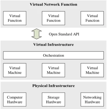
The concept of NFV in mobile core network is replacing specific function hardware with General Purpose Platform (GPP). In this way, the resources, such as computation power and storage, can be virtualized as virtual machines (VM), and the functions can be divided into virtual network functions. Then, the resources and functions can be connected through standard API in more flexible way to meet different performance requirements. Figure 4 shows the architecture of NFV.

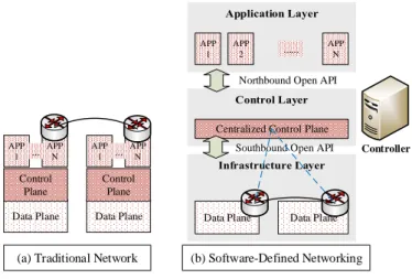
SDN is a new networking paradigm that separates the control modules from the infras-tructure layer to the centralized controllers. Figure 5(a) shows the architectures of traditional network and Figure 5(b) shows the architecture of SDN network. The network devices are self-controlled nodes in traditional network and are responsible for transferring packets only in SDN network. Since the control plane is separated, the network devices communicate with the centralized control plane through southbound Open API , such as OpenFlow [5], and the control plane connect applications through northbound Open API. The switches from differ-ent vendors can easily cooperate with each other through OpenFlow, and thus operators have more choices in selecting infrastructure components. Thanks to SDN, the network adminis-trators can have a global view to manage and control the network more flexibly through the centralized controllers.

In virtualized and programable networks, the network slicing can be adopted to divide GPP into several virtual networks to provide customized network environment for different services and applications. For the complicated 5G network scenarios, this kind of architecture can pro-vide more isolated, flexible and secure networks.

Data Plane Data Plane Data Plane Data Plane Control

Plane

Control Plane

Centralized Control Plane APP

1 APP

N

... APP₁ ... APP_N

(a) Traditional Network (b) Software-Defined Networking APP 1 APP N ... APP 2

Southbound Open API Northbound Open API

Controller

Figure 5: The Comparison of Architecture Between Traditional Network and Software-Defined Networking

1.3

Cloud Radio Access Networks

C-RAN, a novel mobile network architecture, was proposed by IBM in 2010 [6] and China mobile published a white paper to elaborate C-RAN in 2011 [7]. The baseband processing is centralized and shared among sites in a virtualized Baseband Unit (BBU) to optimize the resources utilization of base stations in C-RAN. The deployment cost of small cells, which are used to increase coverage and meet the requirements of 5G in all kinds of environments, can be reduced by adopting C-RAN.

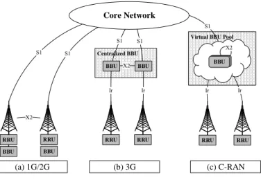
Figure 6 shows the evolution of base station architecture, which can be divided into three steps. As shown in Figure 6(a), traditional macro base station, which Power Amplification (PA), radio frequency (RF) and baseband are integrated inside, is adopted in 1G and 2G. Coaxial ca-bles are used to connect between antenna module and a base station, and X2 interface connects base stations, and S1 interface is defined between a base station and the mobile core networks. The disadvantages of a base station like Figure 6(a) are high deployment cost and high energy consumption for distributed BBUs and their cooling systems. In addition, the computation re-sources are distributed everywhere and can not share among base stations. Therefore, as shown in Figure 6(b), the base station in 3G is separated into radio unit, called Remote Radio Head (RRH) or Remote Radio Unit (RRU), and signal processing unit, called Data Unit (DU) or Baseband Unit (BBU). RRU is responsible for RF and transforming analog signals to digital signals and can be deployed 40 kilometers away from BBU through fiber on Ir interface. Since a BBU can connect several RRUs within 40 Kilometer, computation resources can be shared among RRUs and deployment costs can be reduced. However, the computation resources still can not be shared among BBUs and the computation resources in the low-utilized BBU are wasted. Therefore, C-RAN adopts Virtual BBU Pool, which builds BBUs through GPP in the cloud, to centrally manage computation resources among BBUs. Figure 6(c) shows the archi-tecture of C-RAN, which can reduce the deployment CAPEX and OPEX. The disadvantage of this architecture is the delay between RRUs and Virtual BBU Pool.

Besides, thanks to the centralized architecture, C-RAN is suitable for Coordinated Multi Point (CoMP), which allows a user device to associate multiple base stations simultaneously, and enhanced Inter-cell Interference Coordination (eICIC), which aims at reducing Interference among base stations. So, the advantages of C-RAN also include handling irregular flow and

Virtual BBU Pool Centralized BBU X2 Core Network BBU X2 (a) 1G/2G (b) 3G (c) C-RAN RRU BBU RRU BBU BBU BBU

RRU RRU RRU RRU

Figure 6: The Evolution of Base Station Architecture improving capacity.

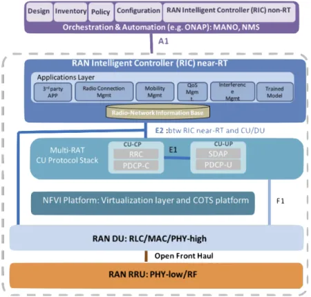
SDN and NFV have spurred significant change in core networks and enable a more agile and less expensive architecture. In the latest years, some theses [8–10] try to bring the concept of SDN/NFV into RAN theoretically. In [9], OpenRAN proposes virtualize RRU, which is con-trolled by SDN, to build software-defined radio access network. Reference [8] adopts C-RAN, which is managed by SDN and NFV. On the top of that, authors connect big data center with core networks to analyze users’ flows and behaviors to improve the performance. The analy-sis results can be applied in resource allocation, devices update, users behavior prediction and network coverage setting through the record of flows and users’ location. Besides, [10] com-bines C-RAN and control protocol in transport layer. Owing to virtualization, the application layer can control radio access and transport simultaneously. Based on this concept, the authors conducts an experiment of two shared-resources services and customized resources allocation. As for industry, C-RAN Alliance was merged with xRAN Alliance, which was founded in 2016 to promote and standardized a software-based and extensible Radio Access Network, in 2018 [11]. The combined Alliance is called Open Radio Access Network (O-RAN) and aims at bring cloud scale economics and agility to the Radio Access Network (RAN). O-RAN pursues the vision of openness to standardized the interfaces and the vision of intelligence to optimize the management for 5G networks. Figure 7 shows the O-RAN Alliance reference architec-ture. BBU is split into Centralized Unit (CU) and Distributed Unit (DU), which are connected through F 1 Interface. CU and DU are placed at different locations according to the operators’ requirements, and only DU is virtualized [12, 13]. To extend SDN concept of decoupling the control-plane (CP) and user-plane (UP) into RAN, CU includes CU-CP and CU-UP, which are connected through E1 Interface as southbound API in Multi-RAT CU Protocol Stack. CU and DU communicate with RAN Intelligent Controller (RIC) near real time through E2 Interface as the northbound API. Non-Real Time (non-RT) control functionality, whose latency is greater than 1 second, and near-Real Time (near-RT) control functions, whose latency is less than 1 second, are decouples and communicate through A1 Interface. The operator members in O-RAN Alliance include AT&T, China Mobile, NTT DOCOMO and several influential operators and vendors all around the world, which lead and drive the transformation of RAN in 5G. Fu-ture RANs will be built on the foundation of virtualized network elements, white-box hardware and standardized interfaces, which embrace O-RAN’s visions. To tame the complexity with

Figure 7: O-RAN Alliance Reference Architecture

the advent of 5G, embed intelligence enables dynamic local radio resource allocation and opti-mizes network-wide efficiency. Therefore, this report tries to investigate the algorithm design and performance evaluation for operator references based on the O-RAN architecture. Since the C-RAN is the origin of O-RAN, the studied architecture is generally called C-RAN in the following descriptions.

二、研究目的與文獻探討

With the advance of MTC and the popularity of smart phone, 20 billion MTC devices and 5.7 billion unique mobile subscribers are expected by 2020 [14] [15]. Compared to high quality multimedia applications and critical applications, smart home devices and mobile phones are more common among people’s life and have been used for several years. Therefore, the de-mands of mMTC is expected to be higher than that of eMBB and URLLC at the early stage of 5G. So, this dissertation focuses on the massive requests scenarios in 5G with C-RAN architec-ture.

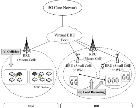
However, massive devices require better association control schemes, which manage the connections between a device and a particular serving base station. Using existing association schemes, the overload demands will meet the physical constrains of the network. Besides, to the best of authors’ knowledge, there are few researches studying user association schemes for massive requests on C-RAN architecture [16]. Figure 8 illustrates three issues, which are all caused by overload demands. When the radio resources are not enough for the demands, collisions happen a lot, which cause low resource utilization and waste device energy as shown in Figure 8(a). In Figure 8(b), when massive devices move among RRUs, load balancing issue

5G Core Network

RRU (Macro Cell)

RRU (Small Cell) or Wi-Fi

RRU (Small Cell) or Wi-Fi M2M H2H MTC Devices RRU (Macro Cell) (a) Collision (b) Load Balancing Virtual BBU Pool

Figure 8: The System Architecture and Studied Issues should be considered to improve the total throughput.

To handle these issues, this dissertation proposes two schemes respectively, which can be implemented in RIC as applications. Since the number of requests exceed the hardware capa-bilities, grouping devices and delaying requests are proposed. The idea of grouping devices can reduce the computation from the number of devices to the number of group in the association schemes. Following subsections briefly describe the schemes and the studied environments.

2.1

Collision

Motivated from mMTC scenario, this dissertation starts from the machine to machine (M2M) traffic of stationary MTC devices. In RAN, the huge amount of devices may cause significant collisions, which occur when more than one device attempts to connect to a channel at the same time. By grouping the devices on the basis of locations, a queue is added in the group to schedule the transportations for the group members by the group leader. In this way, increasing little delay in groups reduces the failed transmissions, which save the power consumption of devices and increase the utilization of radio resources.

2.2

Load Balancing

Then, the movement of devices is considered like Human to Human (H2H) scenario, which characterized by the mobility of human and high data transmission. Therefore, the load bal-ancing issue among multiple base stations should be studied. The devices are grouped by the moving patterns, which assumes that the group members move together, to lower the computa-tion complexity. Besides, benefited from the C-RAN and SDN, an algorithm is proposed at a centralized view to control the association by adjusting the power of RRUs.

2.3

Organization of the Report

This report focuses on the association control of massive requests in 5G C-RAN. Since the increasing number of mobile devices leads to collision, load balancing and ping-pong effect is-sues, this dissertation proposes group-based association control schemes to resolve these issues. Gateway-assisted Two-stage (GATS) Radio Access Scheme is proposed to reduce collisions under a base station with stationary devices. Adaptive Load balancing (ALB) Scheme aim at balancing the data throughput among base stations from moving devices groups.

三、研究方法

3.1

GATS Scheme

In this section, we propose an efficient Gateway-Assisted Two-Stage (GATS) radio access scheme to alleviate the severe congestion for LTE-A MTC. Every MTC device is assumed stationary and belongs to a group.

The Group Establishment procedure is described as follows. Before starting data transmis-sion, all MTC devices are divided into groups according to the location. Initially, no connection exists between MTC devices. When some MTC device wants to send data, it sends a request to eNB to ask for resource blocks. The MTC device successfully sending the first request be-comes the group leader (called MTC gateway). After the MTC gateway finishes transmission, the MTC gateway broadcasts its information, including group number and address, to other MTC devices through a Beacon frame via Zigbee interface. Note that this procedure is only exercised when there is no MTC gateway in the group yet or the gateway is broken.

The MTC devices only receive the beacons with the same group number as that of the devices. When an MTC device does not receive five consecutive beacons from the gateway, the MTC gateway is considered broken. Then the device which wants to send data first after the gateway is broken becomes the new MTC gateway. The procedure is same as the group establishment described above.

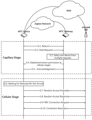
Figure 9 illustrates the message flow of Random Access among MTC device, MTC gateway and eNB. Random Access consists of two stages: Capillary Stage and Cellular stage. Capillary

Stage (Steps G.1-G.5) is Zigbee transmission between MTC device and MTC gateway. Cellular Stage (Steps G.6-G.10) is LTE-A random access procedure between MTC device and eNB.

Step G.1. The MTC gateway broadcasts its information through a Beacon frame.

Step G.2. The MTC device sends a request to inform MTC gateway that MTC device attempts

to initiate a random access procedure.

Step G.3. MTC gateway use a queue to record the requests of random access from devices.

Only one device is granted to initiate a random access procedure per time slot.

Step G.4. MTC gateway sends a data frame to the selected MTC device, which is used to permit

the device to enter cellular stage.

Step G.5. MTC device sends acknowledgment message to MTC gateway.

Step G.6. After being permitted, the MTC device uses the standard slotted access scheme to

calculate its dedicated time slot number by its International Mobile Subscriber Identity (IMSI). Then the MTC device keeps silent until the arrival of the dedicated time slot.

G.6. Waiting for Dedicate RA-Slot Arrival

G.3. Select one device from multiple requests G.4. Data(transmission permission at cellular stage) Zigbee Network RAN MTC Device MTC Gateway eNodeB Capillary Stage Cellular Stage

Figure 9: Message Flow of Gateway-Assisted Two-Stage Random Access

Steps G.7-G.10. Same steps as basic scheme proposed in 3GPP TS 36.300 [22] for an MTC

device to request for resource blocks from eNB.

The major motivation to separate the single stage random access in basic scheme is to pass collision to the gateway, and thus reduce the overall collision probability. Furthermore, sep-arating a single stage into two stages substantially incurs more message delay. To sum up, GATS alleviates the collision probability by sacrificing some message delay. Note that MTC gateway only “assists” LTE-A random access by random access at capillary network. Data are transmitted directly between MTC device and eNB, not relayed by MTC gateway.

Note that, compared to the basic scheme, the devices in our proposed method indeed incur extra cost on Zigbee. Zigbee used in capillary network can be replaced by communication techniques used in LTE-A, such as device to device (D2D) communication, to avoid extra cost. In this case, the MTC devices only need to be equipped with LTE-A chips. However, some co-channel issues (e.g., interference) need to be considered at the same time. To focus on the effect of two-stage random access, we adopt different radio technologies in the two stages, and leave the co-channel condition as future work. In this section, we derive the collision probability and expected queue size for the GATS scheme. We adopt most system parameters from [25]. When a message arrives from application layer, the MTC device attempts to access the radio resources at the next random access slot. Assume that the message arrivals from application layer at each MTC device form a Poisson process with rate λ. The random access slot is scheduled every T seconds.

For simplicity, we assume that the MTC devices that collide at a random access slot resume at the next random access slot. This assumption is relaxed later in simulation experiments. In practice, MTC devices are usually implemented by Arduino UNO, which has at least 32K

bytes of Flash memory [52, 53]. Since the network address of Zigbee requires 16 bits [54], the maximum queue size of 16000 devices is allowed in the GATS scheme. In our simulation experiments, there are at most 2700 devices in a group. In this case, 32K bytes of Flash memory is quite sufficient.

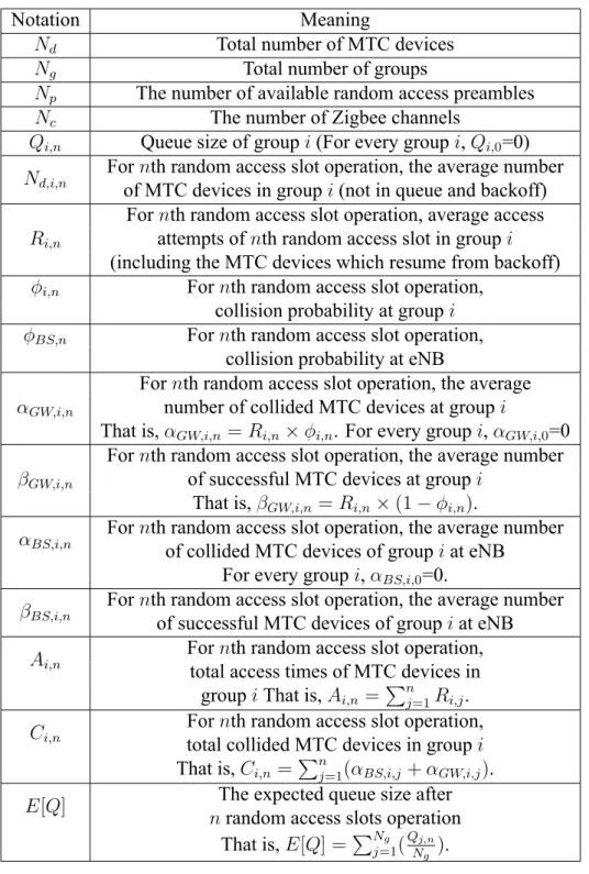
e derive the expected queue size E[Q] and overall collision probability ϕ. The notations are listed in Table 1.

The collision occurs if more than one MTC device transmits the same random access pream-ble in the same random access slot. According to [55], the collision probability is given by

Pr[collision] = 1− e−γL (1)

where γ is the number of access attempts per second, and L is the total number of access op-portunities per second. We assume that the deployment of MTC devices in a cell is uniformly distributed. Therefore, for initialization (1st random access slot), the average number Nd,i,1 of

MTC device in group i is expressed as the fraction of total number Ndof MTC devices and total

number Ng of groups. That is,

Nd,i,1 =

Nd

Ng

(2)

Ri,n is the average number of access attempts of nth random access slot in group i, which is

expressed as the average number of access attempts of MTC devices not in queue adds the number of MTC devices resume from backoff. The equation is expressed as

Ri,n= Nd,i,n× λ × T + αBS,i,n−1+ αGW,i,n−1 (3)

There is no collided MTC device at the beginning. Therefore, we define both αGW,i,0and αBS,i,0

as 0. According to (2) and (3), we can get the initial average access attempts in group i

Ri,1 = Nd,i,1× λ × T (4)

In the GATS scheme, a collision possibly occurs at an MTC gateway or an eNB.

• Capillary Stage: The MTC devices (not in queue and backoff) may send new access requests to an MTC gateway via zigbee.

• Cellular Stage: The MTC devices (in the front of queue in group gateway) perform random access procedure to the eNB.

The collided MTC devices at both Capillary stage and Cellular stage then perform backoff. Since the backoff time is a fixed value, all the collided MTC devices resume in the next random access slot. However, the MTC devices that resume from backoff randomly choose a preamble respectively, such that those collided MTC devices might not collide again. At capillary stage, the network of MTC devices is a star topology and beacon enabled network. In [56], the slotted CSMA/CA mechanism for Zigbee is analyzed. The derivation in [56] is similar to that in [55] except for the backoff scheme. Since we assume a simple backoff scheme (i.e., all the collided devices resume in the next slot) in our analytic model, the derivation for collision probability becomes quite similar. Therefore, to express the collision probability at MTC gateway, we use the same equation from (1) by changing preamble number to Zigbee channel number. That is,

ϕi,n= 1− e

−Ri,n

Table 1: Notations for GATS Scheme Notation Meaning

Nd Total number of MTC devices Ng Total number of groups

Np The number of available random access preambles

Nc The number of Zigbee channels

Qi,n Queue size of group i (For every group i, Qi,0=0) Nd,i,n

For nth random access slot operation, the average number of MTC devices in group i (not in queue and backoff)

Ri,n

For nth random access slot operation, average access attempts of nth random access slot in group i (including the MTC devices which resume from backoff)

ϕi,n For nth random access slot operation,

collision probability at group i

ϕBS,n For nth random access slot operation,

collision probability at eNB

αGW,i,n

For nth random access slot operation, the average number of collided MTC devices at group i

That is, αGW,i,n = Ri,n× ϕi,n. For every group i, αGW,i,0=0 βGW,i,n

For nth random access slot operation, the average number of successful MTC devices at group i

That is, βGW,i,n= Ri,n× (1 − ϕi,n). αBS,i,n

For nth random access slot operation, the average number of collided MTC devices of group i at eNB

For every group i, αBS,i,0=0. βBS,i,n

For nth random access slot operation, the average number of successful MTC devices of group i at eNB

Ai,n

For nth random access slot operation, total access times of MTC devices in

group i That is, Ai,n=

∑n j=1Ri,j. Ci,n

For nth random access slot operation, total collided MTC devices in group i That is, Ci,n=

∑n

j=1(αBS,i,j+ αGW,i,j). E[Q] The expected queue size after

n random access slots operation

That is, E[Q] =∑Ng j=1(

Qj,n Ng ).

For the collision probability at eNB, L is the product of the number of available random access preambles and the number of random access slots per second. From (1) and similar derivation of ϕi,n, the collision probability at eNB is derived as

ϕBS,n= 1− e

−λ×Ng×T

Np ₍₆₎

In the GATS scheme, for each group, only one MTC device in queue is permitted to send request to eNB in a random access slot. Therefore, the number of collided MTC device is the product of 1 (MTC device) and collision probability at eNB, if current queue size is larger or equals to 1. If the current queue size is less than 1 and larger or equal to 0, αBS,i,n= 0. The current queue

size is the sum of the queue size in last time slot and the number of successful MTC devices at Capillary stage. That is,

αBS,i,n =

{

1× ϕBS,n, if Qi,n₋₁+ βGW,i,n≥ 1

0, if 0≤ Qi,n₋₁+ βGW,i,n< 1

(7) The number βBS,i,n of MTC device which transmits request successfully is the product of

1 (MTC device) and access success probability at eNB, if current queue size is larger or equals to 1. If the current queue size is less than 1 and larger or equal to 0, βBS,i,n= 0. That is,

βBS,i,n=

{

1× (1 − ϕBS,n), if Qi,n−1+ βGW,i,n ≥ 1

0, if 0≤ Qi,n₋₁+ βGW,i,n < 1

(8) If current queue size is larger or equal to 1, the MTC device in the front of queue sends request to eNB. Therefore, the queue size of group i is subtracted by 1. If current queue size is smaller than 1, the queue size of group i still equals to current queue size. That is,

Qi,n=

{

Qi,n−1+ βGW,i,n− 1, if Qi,n−1+ βGW,i,n≥ 1

Qi,n−1+ βGW,i,n, if 0≤ Qi,n−1+ βGW,i,n< 1

(9) When the two-stage radio access in a random access slot finished, the MTC devices’ access attempts in a random access slot is separated into two parts: (i) attempts in queue and (ii) attempts in backoff (because of collision at MTC gateway and eNB). And the average number

Nd,i,nof MTC devices in group i changes, it is expressed as

Nd,i,n = Nd,i,n−1− Nd,i,n−1× T + βBS,i,n−1, n≥ 2 (10)

From (2) and (10), we have

Nd,i,n=    Nd,i,n−1− Nd,i,n−1× λ × T +βBS,i,n−1, n ≥ 2 Nd Ng, n = 1 (11)

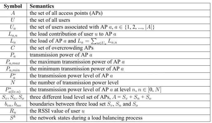
Table 2: Notations for ALB Scheme

Symbol Semantics

A the set of all access points (APs)

U the set of all users

Ua the set of users associated with AP a, a∈ {1, 2, ..., |A|} La,u the load contribution of user u to AP a

La the load of AP a and La=

∑

u∈UaLa,u C the set of overcrowding APs

Pa transmission power of AP a

Pa,max the maximum transmission power of AP a

Pa,min the minimum transmission power of AP a

P_a∗ the transmission power level of AP a

N the number of transmission power level

P_a(lv.n)∗ the transmission power level of AP a at level n, n∈ [0, N]

Sv, Sn, So three different load level set of APs, A = Sv+ Sn+ So bvn, bno boundaries between three load set Sv, Snand So

Ru the RSSI value of user u

Sk _{the network states during a load balancing process}

After n random access slots, the overall collision probability ϕ is expressed as

ϕ = Ng ∑ i=1 Ci,n Ai,n × 1 Ng = Ng ∑ i=1 ∑n j=1(αGW,i,j+ αBS,i,j) ∑n j=1Ri,j × 1 Ng (12)

3.2

ALB Scheme

The notations used in our scheme are shown in Table 2. We consider an IEEE 802.11 WLAN with a set of APs, which is denoted by A, and |A| indicates the number of APs. All APs are attached to a wired infrastructure and an OpenFlow controller. In our scheme, we focus on the transmission power of AP beacon messages since beacon messages are used for AP association. We denote transmission power of AP a as Pa. According to the configuration and

capabil-ity, each AP has its maximum and minimum transmission power, which are denoted as Pmax

and Pmin respectively. Each AP also provides several transmission power levels from 0 to N ,

denoted by P_a(lv.n)∗ . We denote P_a(lv.0)∗ = P_a,min∗ as the minimum power level of AP, and sim-ilarly we denote P_{a(lv.N )}∗ = P_a,max∗ as the maximum power level. For normal commercial AP products, the transmission power level configuration follow that

P_a∗ = logγ(Pa) , γ = N

√

Pmax

Pmin

P_a(lv.n)∗ is a geometric series which can be expressed as

P_a(lv.k)∗ = P_a(lv.k∗ ₋₁₎∗ γ (14)

P_a(lv.k)∗ = P_a,min∗ ∗ γk, k∈ [0, N]. (15)

Here are some assumptions in our scheme. First, the interference between adjacent cells is assumed to be ignored. Second, the deployment of APs ensures that every user can be still covered under network coverage even if all APs are configured to the minimum transmission power Pmin, Third, each user associates with at most one AP at any time.

Once a mobile device enters a WLAN, it listens every channel for all beacon messages from APs. Then, it associates with the AP which has the strongest RSSI, which is influenced by the beacon transmission power and the distance between AP and device. In our system, the RSSIs from users are collected by APs and reported to the controller through OpenFlow protocol. Besides, each AP collects its load La and the load contribution of its users La,u to controller

periodically. In this way, the controller knows the association relationships between users and APs and the load of APs. from a global view of the whole networks.

U is denoted as the set of all users in the network coverage area, and|U| is total number of

users in U . Ua is the set of users associated with AP a. If a large amount of user association

requests are sent to an AP in a short time, the AP become overloaded. To tame the complexity of computation, we consider the group arrival cases. In our analysis, all users follow a group mobility model, which means that the users usually move together from one place to another in several groups.

Benefited from the global view of the controller, our model can coordinate the load of all APs and take the users’ load contributions into consideration. The controller records the load contribution of user u to AP a, La,u by considering the load report from APs. Each AP can

provide optimal bandwidths to its associated users in our model.

3.2.2 Flowcharts

In this subsection, we present the ALB scheme procedures and the flowcharts of collecting association reports and managing mechanism.

Figure 10 illustrates the message flow of association control between users, APs and con-troller. In this example, user is in the coverage of AP 1 and AP 2, and AP 1 is closer to user than AP 2.

Step 1. AP 1 and AP 2 send Beacon Message to the user periodically.

Step 2. AP 1 and AP 2 report their load and association events to controller. In OpenFlow

protocol, association event can be transmit in Packet_In message and the load of AP can be transmitted in Port_Status message.

Step 3. Controller periodically checks all of the AP load and integrates all association event

reports of APs. Then controller inputs these information to execute Adaptive Load Bal-ancing algorithm.

Step 4. Based on the result of Step 3, controller sends Beacon-Config messages through

Set-Config message in OpenFlow to APs. In this case, controller decreases the AP 1 beacon power lower and increases the AP 1 beacon power lower.

User AP 1 AP 2 Controller

4. Set Lower Beacon Power 2. Report Load and Association Events 1. Beacon Message 1.Beacon Message 7. Association Response 8. Authentication Request 9. Authentication Response 6. Association Request

2. Report Load and Association Events

5. Beacon Message

4. Set Higher Beacon Power 5. Beacon Message

3. Checking All AP Loads and Run Adaptive Load Balancing Program

Figure 10: Message Flow of Association Control

Step 7-9. The user sends association request to AP 2, which has the highest RSSI. After

re-ceiving an association response from AP 2, user sends an authentication request to AP 2. When AP 2 sends back authentication response, the connection between user and AP 2 is established.

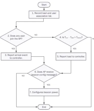
To collect association reports, APs need to report its user association events and load in real time. Figure 11 shows the flow chart of AP reporting mechanism, and the steps are described below.

Step 1. Each AP records the user RSSI, user association list and its load periodically. All APs

receive RSSIs in every authentication frames from their users.

Step 2. If there is a new user associating with the AP, go to Step 3. Otherwise, go to Step 4. Step 3. The AP sends the user RSSI to the controller. Then go to Step 6.

Step 4 and 5. If there is no new arrival in Step 2, the AP reports its load to controller

periodi-cally.

Step 6. After sending report messages to controller, the AP would receive a Beacon-Config

message from the controller.

Step 7. The AP configures its beacon transmission power.

Figure 12 illustrates the flow chart of the controller management mechanism, and following are the descriptions of steps.

Step 1. The controller receives arrival events and load messages from APs.

Step 2. The number of new arrival events is added into the arrival counting table. Then the

Start

6. Does AP receive

beacon-config message?

3. Report arrival event to controller.

7. Configures beacon power.

YES

1. Record load and user association list.

2. Does any user join the AP?

YES

4. Is Tcur–Tlast > Texpiry?

NO

NO

5. Report load to controller.

YES

NO

End

Figure 11: Flow Chart for AP Reporting Mechanism

Step 3. The controller compares the number of current arrival events with the past. When an

AP exceeds the threshold of arrival events, it has a high risk of overcrowding. At this time, the controller gives the AP a predicted load value and then go to Step 6.

Step 4. The controller classifies all APs into three load levels: vacant, normal and

overcrowd-ing. According to the levels, the APs are added into (Sv, Sn and So) respectively. The bvn and bnodenote the boundaries between these levels.

Ll,a =    v, for La≥ bvn n, for bno ≤ La< bvn o, for La< bno    (16) a∈    Sv, for Ll,a = v, Sn, for Ll,a = n, So, for Ll,a = o,    (17)

Step 5. This procedure ends when there is no AP changing to overcrowding state So.

Step 6. The controller calculates the adjustments of APs according to the load balancing

algo-rithm which is described in next subsection.

Start

3. Is group arrival event happened?

1. Receive arrival event and load from APs.

7. Send beacon-config message to APs . 6. Run load balancing

algorithm.

YES

NO

2. Calculate the arrival increase.

4. Classify APs into three kinds of load state.

(Sv, Sn and So) 5. Does any AP change to So? YES NO End

Figure 12: Flow Chart for Controller Management Mechanism

3.2.3 Load Balancing Algorithm

In this subsection, the load balancing algorithm in ALB scheme is elaborated. As the descrip-tions in subsection 3.2.1 and 3.2.2, the association reladescrip-tionship, RSSIs of users and load of APs are all collected by the controller. Based on the information above and the concept of Cell Breathing, we proposes an algorithm to calculate the optimal power levels for all APs from a global vision of whole wireless network.

Figure 13 is the pseudo code of ALB algorithm, which is an iterative greedy algorithm. Before executing the algorithm, the beacon power levels of all APs are initialized to the maximal power level. The first network state S0is also initialized to the summations of all AP utilizations before any power adjustment. First, the algorithm finds the most overcrowding AP and adds this AP into overcrowding set C and sets its power one level down. In the meanwhile, the adjustments are recorded in a stack structure. Every time the most overcrowding AP sets down beacon power level, the algorithm updates the network states by simulating the association relationship between APs and users. Each state is compared with previous states to find the optimal state. Until the iteration ends, the algorithm sets all AP beacon power level according to the optimal state.

The iteration in two conditions. The first condition is that the overcrowding set C is equal to AP set A, which means every AP is adjusted. If the iteration continues, the new network state won’t outperform the previous state. At this time, all AP are overcrowding and can’t offload users from other overcrowding AP. The other condition happens when any AP beacon power is adjusted to the minimum level. Since the AP can not level down their beacon power anymore, the AP is still the most overcrowding AP.

The time complexity of the algorithm is O(|A| × N). Based on the tolerant of delay, the operators can deploy the suitable number of APs. If the mobility of users in the area is too high, the algorithm will executed too frequently. In this case, thanks to the flexibility of C-RAN, APs

Figure 13: Adaptive Load Balancing Algorithm

can be divided in groups dynamically and algorithm run for groups separately to reduce the complexity. If the number of power level N increases, the results can be calculated in higher granularity. The effect of granularity on throughput is analyzed in the next chapter.

四、結果與討論

4.1

GATS Scheme

In this section, we evaluate the performance of our scheme with simulation experiments. Sim-ulation model for GATS is described in [57]. Readers are referred to [57] for description of the simulation model. The system parameters for the GATS scheme are listed in Table 3. We refer to [25] and [58] for most parameter settings.

4.1.1 Effects of Ndon ϕ and E[Q]

Figure 14 illustrates the relation between the number of devices Ndand overall collision

proba-bility ϕ. Firstly, to verify the correctness of simulation program and mathematic model, Figure 14 show the simulation results drawn by dots are consistent with the mathematic results drawn by lines. It is observed that the collision probability in the GATS scheme is almost equal to that of basic scheme when Nd< 2048.. When Ndis greater than 8192, significant rise is observed

in terms of collision probability because of the increasing requests. In this congested situation, GATS scheme tries to offload the collisions to gateway for avoiding collision at eNB. When

Nd= 32768, ϕ is only 62% in GATS scheme and almost 99% in basic scheme. GATS scheme

reduces about 99%− 62% = 37% collision and the probability of collision at gateway is even less than 5% .

Table 3: Simulation Parameters for GATS Scheme Parameter Assumption Total number of active MTC devices (Nd) 35670

Cell bandwidth 5 MHz Cell radius 0.5 km PRACH configuration index 6

MTC devices deployment Uniform distribution Simulation time 1000000 ms Number of Zigbee channels 16

Number of preambles 54 Period of RACH 5 ms Backoff indicator [24] [0, 960] ms 10% 20% 30% 40% 50% 60% 70% 80% 90% 100% φ 32 64 128 256 512 1024 2048 4096 8192 16384 32768 Nd ⊳: Basic Scheme(Simulation)

•: GATS Scheme Device to GW(Simulation) ⋄: GATS Scheme GW to eNB(Simulation) ⋆: GATS Scheme total(Simulation)

. . ... ... . . ... . . ... Basic Scheme(Analytic)

GATS Scheme Device to GW(Analytic) GATS Scheme GW to eNB(Analytic) GATS Scheme total(Analytic)

. ... ... ... ... . . ... ... ... . . ... . . . . . . . ... . ... . . . . . . ... . ... . . . . . ... ... . . . . . ... ... . . . . ... . . . . . . . . . .... . . . . ... . . . . . . . . ... . . . ... . . . . . . . . ... . ... ⊳ ⊳ ⊳ ⊳ ⊳ ⊳ ⊳ ⊳ ⊳ ⊳ ⊳ ... •...•...•...•...•...•...•...•...•... • • ... ... . ... ⋄ ⋄ ⋄ ⋄ ⋄ ⋄ ⋄ ⋄ ⋄ ⋄ ⋄ . ... ⋆ ⋆ ⋆ ⋆ ⋆ ⋆ ⋆ ⋆ ⋆ ⋆ ⋆ Figure 14: Effects of Ndon ϕ (λ = 0.3, Ng = 64)

0 500 1000 1500 2000 2500 3000 E[Q] 0 10000 20000 30000 40000 50000 60000 70000 80000 90000 100000 N_d • : Ng= 32 ⋄ : Ng= 64 ⊳: Ng= 128 . . ... • • • • • • • • • • . . ... ⋄ ⋄ ⋄ ⋄ ⋄ ⋄ ⋄ ⋄ ⋄ ⋄ . . ... ⊳ ⊳ ⊳ ⊳ ⊳ ⊳ ⊳ ⊳ ⊳ ⊳

Figure 15: Effects of Ndon E[Q] (λ = 0.3)

Figure 15 illustrates effects of the number of devices Nd and the number of groups Ng on

expected queue size E[Q]. In the GATS scheme, only one device in a group is permitted to send request to eNB in a random access slot. Therefore, if more than one device send requests to group leader (MTC gateway), the queue size in the group rises constantly. When Ndis less

than 10000, the demands of requests are still affordable and E[Q] = 0. The congestion starts when Nd > 10000, and the figure shows that E[Q] is proportional to Nd intuitively. When Ng increases, the number of devices per group decreases and E[Q] decreases. Operators can

refer this results to deploy suitable number of devices and number of groups according to the expected maximum queue size. For example, if the operator tries to limit the queue size to 1000, then the networks can afford about 40000 devices with 32 groups or 80000 devices with 64 groups.

4.1.2 Effects of λ and Ngon RA-slot Utilization

In this subsection, Figure 16 illustrates the RA-slot utilization, which indicates the ratio of the number of successful requests and the number of preambles, with different Ng. When collision

occurs, the collided RA-slot can not be used by any MTC device. As a result, utilization of RA-slot decreases as collision probability increases. Besides, Basic Scheme, GATS Scheme and Tsai’s Method are compared in the following experiments. In GATS Scheme, at most one device per group sends the request and competes with other devices from other group. In Tsai s Method, each group has the specific grant time interval, and so the device competes with its group members. When Ng = 1, three schemes behave the same. When Ng increases and the

device number in a group is close to 1, the GATS Scheme behaves the same as Basic Scheme. When the arrival rate of requests is small and there is almost no collision (λ = 1), GATS Scheme have the same RA-slot Utilization as Basic Scheme. However, when Ng increases,

Tsai’s Method grants more unused time intervals so that RA-slot Utilization decreases. In con-gested situation (λ = 3), the RA-slot utilization of GATS Scheme increases and then decreases as Ngincreases. If Ngis small, the collision mainly occurs at the MTC gateway. Conversely, if Ng is large, the collision mainly occurs at the eNB like Basic Scheme. That is, Ng is suggested

to be set near the number of preambles in GATS scheme to achieve the maximum RA-slots Utilization. The figure shows that the best RA-slot utilization, which is about 37%, is observed

0.1 0.2 0.3 0.4 R A -s lo t U t iliz a t io n 4 36 100 196 324 484 676 900 1156 1444 N_g

⋄: Basic Scheme •: GATS Scheme ⋆: Tsai’s Method

. ... λ= 0.3 ... λ= 0.2 ... λ= 0.1 . ... ⋄ ⋄ ⋄ ⋄ ⋄ ⋄ ⋄ ⋄ ⋄ ⋄ . . . . . ... • • _• • • _• • • • • . ... ⋆ ⋆ ⋆ ⋆ ⋆ ⋆ ⋆ ⋆ ⋆ ⋆ . ... ⋄ ⋄ ⋄ ⋄ ⋄ ⋄ ⋄ ⋄ ⋄ ⋄ . . . . . ... . . . . . ... . . . . . . ... . . . . . . ... . . . . . . . . ... . ... . . . . ... . . . . . . . ... . . . . . . ... ... . ... . ... . . ... . . . ... ... . ... ... ... . . . ... . ... . . . . ... . . . . ... . ... . . . ... . . . . ... ... . . . ... ... . . ... ... • • • • • _{• •} • • • . ... ... . ... . ... ... . . ... ... . ... . . ... . . ... . ... ... ... ... . . ... ... ... ... . ... . ... ... ... ... . ... ... .... ⋆ ⋆ ⋆ ⋆ ⋆ ⋆ ⋆ ⋆ ⋆ ⋆ ... ⋄ ⋄ ⋄ ⋄ ⋄ ⋄ ⋄ ⋄ ⋄ ⋄ . . . . . . . . . . . . . . . . . . . . . . . . . .. ... • • • • • • • • • • ... ... ... . ... .... ⋆ _⋆ ⋆ ⋆ ⋆ ⋆ ⋆ ⋆ ⋆ ⋆

Figure 16: Effects of Ngon RA-slot Utilization

when Ng = 64 for GATS scheme and when Ng ranges from 300 to 500 for Tsai’s Method.

4.1.3 Effects of λ and Ngon Access Success Probability

In this subsection, we investigate the access success probability, which is expressed as ratio of the total number of success requests and the total number of requests, with different Ng.

Figure 17 shows that, in GATS Scheme, the access success probability decreases as Ng

in-creases. When λ = 0.3 and Ng is small, the access success probability decrease slightly. The

slightly decrement is due to the large number of requests in a group, such that severe collision occurs at MTC gateway. When Ng = 64 and λ = 0.3, the access success probability is about

98%, which improves about 98%−12%

12% = 716% than the Basic Scheme. When λ = 0.1, because

of the number of requests in a group becomes smaller such that the collision probability is quite small. Therefore, the access success probability of the GATS scheme and the basic scheme are about the same. The obvious improvement is observed with larger λ in the GATS scheme. Fur-thermore, nearly 100% access success probability is observed with Ng < 64 in GATS scheme

and with Ng > 676 in Tsai’s Method.

4.1.4 Effects of λ and Ngon Average Message Delay

In this subsection, we investigate the average message delay with different Ng through

Fig-ure 18.

In GATS Scheme, the average message delay decreases as Ng increases. As Ng increases,

the number of MTC devices in a group decreases, and thus the possible waiting time (including backoff time in case of collision and the queueing time) at the gateway decreases as well. When

Ng = 64 and λ = 0.3, the average message delay is around 5000 ms which has about 150% overhead compared to basic scheme . However, in Figure 17, the access success probability improves 716%. According to [59], MTC allows extending sleep cycles to several minutes for delay-tolerant MTC applications. Therefore, the increment of average message delay is

20% 40% 60% 80% 100% A cc es s S u cc es s P ro b a b ilit y 4 36 100 196 324 484 676 900 1156 1444 N g

⋄: Basic Scheme •: GATS Scheme ⋆: Tsai’s Method

. ... λ= 0.3 ... λ= 0.2 ... λ= 0.1 . ... ⋄ ⋄ ⋄ ⋄ ⋄ ⋄ ⋄ ⋄ ⋄ ⋄ . ... • • • • • _{• •} • • • . ... ⋆ ⋆ ⋆ ⋆ ⋆ ⋆ ⋆ ⋆ ⋆ ⋆ . ... ⋄ ⋄ ⋄ ⋄ ⋄ ⋄ ⋄ ⋄ ⋄ ⋄ . ... . . ... . . ... ... . ... . . . ... . . . ... . . . ... . . . . ... . . . . ... . . . . ... . ... . . . . ... . . ... . ... ... • • • • • _{• • •} • • . ... ... . ... ... . . ... . ... . . . ... . . ... . . ... . . ... ... ... ... . ... . ... . ... ... . ... ⋆ ⋆ ⋆ ⋆ ⋆ ⋆ ⋆ ⋆ ⋆ ⋆ ... ⋄...⋄...⋄...⋄...⋄...⋄...⋄...⋄...⋄...⋄... •...•...•...•...•...•...•...•...•...•... ⋆ ⋆ ⋆ ⋆ ⋆ ⋆ ⋆ ⋆ ⋆ ⋆

Figure 17: Effects of Ngon Access Success Probability

worthwhile for the improvement of access success probability.

In Tsai’s Method, the length of grant interval cycle becomes longer as Ng increases. The

message delay is mainly caused by the number of retransmissions and the length of cycle. To achieve the best RA-slot Utilization in congested situation (λ = 0.3), the average message delay is about 5800 ms in Tsai’s method (Ng = 484) and is about 5000 ms in GATS Scheme.

4.1.5 Discussion about Power Consumption

Power consumption is an important issue for MTC. In GATS, both group establishment and RACH procedures are subject to energy consumption constraints. Since the group establishment is exercised only once until the gateway is broken, the consumed power could be neglected.

Compared to the basic scheme, GATS scheme needs extra energy to send messages at cap-illary stage, but GATS scheme reduces re-transmission count caused by collision at cellular stage. According to [60], an MTC device needs 249.59 ms·mA to send a request with ACK in the capillary stage. As for the cellular stage, the whole random access procedure takes 19 ms with 50 mW power consumption for both RX and TX [61]. Hence, taking a normal 1.5V AAA battery for example, a single random access procedure costs about 50_1.5×19 = 633 ms·mA. When

λ = 0.3 and Ng = 32 in Figure 17, the access success probability for GATS is 100%, while

the success probability for the basic scheme is 30%. For a transmitted message, GATS scheme incurs power 249.59 + 633 = 882.59 ms·mA, while the basic scheme incurs power 633_0.3 = 2110

ms·mA (that is, the average number of retransmission is_0.31 = 3.33). In this case, GATS scheme

saves (2110₂₁₁₀−882.59) = 58% of power consumption as compared to the basic scheme.

4.2

ALB Scheme

To evaluate the performance of load balancing, this section compares Strongest-Signal-First (SSF), Least-Load-First (LLF), Cell-Breathing and ALB Scheme.

100 1000 10000 100000 A v er a g e M es sa g e D ela y (m s) 4 36 100 196 324 484 676 900 1156 1444 N g

⋄: Basic Scheme •: GATS Scheme ⋆_{: Tsai’s Method}

... λ= 0.3 ... λ= 0.2 ... λ= 0.1 ... ⋄ ⋄ ⋄ ⋄ ⋄ ⋄ ⋄ ⋄ ⋄ ⋄ . ... • • • • • • • • • • ... ⋆ ⋆ ⋆ ⋆ ⋆ ⋆ ⋆ ⋆ ⋆ ⋆ ... ⋄ ⋄ ⋄ ⋄ ⋄ ⋄ ⋄ ⋄ ⋄ ⋄ . ... . . ... . . . ... ... . . ... ... ... . ... ... ... • • • • _{• • • • • •} ... ⋆ ⋆ ⋆ ⋆ ⋆ ⋆ ⋆ ⋆ ⋆ ⋆ ... ⋄ ⋄ ⋄ ⋄ ⋄ ⋄ ⋄ ⋄ ⋄ ⋄ . . . . . . . . . . . . . . . . . . . . . . . . . ... • • • • • • • • • • ... ... ... ... ⋆ ⋆ ⋆ ⋆ ⋆ ⋆ ⋆ ⋆ ⋆ ⋆

Figure 18: Effects of Ngon Average Message Delay

4.2.1 Simulation Model

Table 4 shows simulation parameters used in the experiments according to existing Cell-Breathing method in literature [50]. Each experiment lasts 10000 seconds on NS3. The simulated net-works include 20 APs, which are all support IEEE 802.11g standard and equipped with 54 megabits per second backhaul link. These APs locate in 550∗450m2area and are arranged into four lines for five APs per line as shown in Figure 19. The distance between two adjacent APs is set to 100 meters, and those APs are 75 meters far from the simulated area border. In order to ensure that all users are in the coverage of APs, the minimum transmission distance is 75 meters. Table 5 lists the relationship between SNR and bit rate to determine the transmission bit rate between users and APs.

As for user mobility model, Reference Position Group Mobility model (RPGM) generated from BonnMotion tool is adopted to generate three cases of user number, including 100, 250 and 400. These users are divided into two groups and follow the group mobility with heavy connection demands.

Table 4: Simulation Parameters for ALB Scheme Parameters Values

Simulated Time 10000s

Simulated Area 550 * 450 m^2 MAC Protocol IEEE 802.11b Transmission Range [75, 150] m Adjacent AP distance 100 m AP Number 20

User Number 100, 250,400

Mobility Model Reference Position Group Mobility (RPGM) Moving Speed [0.5, 1.5] m/s

Figure 19: System Architecture in ALB Scheme Table 5: Traffic Bit Rate

Bit Rate (Mbps) SNR(dB) Distance (m) 11 ≧ 9 50 5.5 ≧ 5 80 2 ≧ 3 120 1 ≧ 1 150

4.2.2 Performance of APs

The performance of APs are measured by La, which is the sum of associated user throughput,

and La,u), which is the product of user bandwidth and user data rate. The user bandwidth is

assumed to be allocated to users fairly in an AP. The user data rate can be derived from user SNR or distance with AP in Table 5.

Figure 20 shows the total AP load during simulation time. Since this dissertation focuses on improving performance in congested scenario, it’s better to have higher load of APs. The figure shows that ALB Scheme outperforms other traditional methods in the period of the whole experiment. The following experiments shows a closer look to each AP in terms of average AP load and user number.

Figure 21, 22 and 23 show the average load of all APs with 100, 250 and 400 users respec-tively. In the case of 100 users, there are two groups with average 50 users, who are all less than 50 meters from their group center. In the case of 250 users, there are five groups with average 50 users, who are all less than 50 meters from their group center. In the case of 400 users, there are two groups with average 200 users, who are all less than 100 meters from their group center. Table 6 calculates the summation of the average load in the above three cases.

In Figure 21, the X-axis represents the index of APs, which are sorted by the average load in increasing order. In SSF, some APs are heavily congested and some APs are vacant. The curves

0

200

400

600

800

1,000

20

40

60

80

100

Simulation Time (seconds)

T

o

ta

l

A

P

L

o

a

d

(M

b

p

s)

Figure 20: The Total AP Load (400 Users)

of ALB Scheme, LLF and Cell-Breathing are more gently than the curve of SSF. Although the curve of Cell-Breathing is the most gently one, the sum of its average load is the least. As Table 6 shows, the load of our scheme improves 11% compared to SSF and 346% compared to Cell-Breathing. When the network is not so congested, Cell-Breathing does not tend to adjust AP beacon power levels to the optimal result because of the limited knowledge of network situation. When the number of user increases in Figure 22 and 23, the population distribution be-comes more crowded and imbalanced. Figure 23 illustrates that the gap between SSF and Cell-Breathing is smaller than the gap in Figure 22. This variation infers that Cell-breathing performs better in the congested scenario. However, ALB Scheme still outperforms Cell-breathing and other methods. In congested situation, ALB Scheme improves around 26% compared to Cell-breathing and 136% compared to LLF in terms of AP average load.

Figure 24 illustrates the distribution of the average user number in all APs. The X-axis Table 6: Summary of the AP Load

1 2 3 4 5 6 7 8 9 10 11 12 13 14 15 16 17 18 19 20 0 1 2 3 4 5 6 7 Index of AP (Sorted) A v er a g e L o a d (M b p s) SSF LLF Cell-Breathing ALB

Figure 21: The Average Load of All APs (100 Users)

1 2 3 4 5 6 7 8 9 10 11 12 13 14 15 16 17 18 19 20 0 2 4 6 8 Index of AP (Sorted) A v er a g e L o a d (M b p s) SSF LLF Cell-Breathing ALB

1 2 3 4 5 6 7 8 9 10 11 12 13 14 15 16 17 18 19 20 0 2 4 6 8 10 Index of AP (Sorted) A v er a g e L o a d (M b p s) SSF LLF Cell-Breathing ALB

Figure 23: The Average Load of All APs (400 Users)

represents the index of APs sorted by the average user number in increasing order. In terms of average users number, SSF is obviously the most imbalance method because all users pre-fer connecting with the strongest signal AP (i.e. the nearest AP). If there are too much users connecting to an AP at the same time, these users have poor bandwidth to transmit data and the radio resources in the idle AP are wasted. The other three methods balance the users number among APs very well.

4.2.3 Effects on Users

In this subsection, the average user RSSI and average throughput are measured to evaluate the effects on users. The RSSI is calculated by the following formula, and Antenna gain is 5 dBi.

RSSI = Signal− P athloss + AntennaGain (18)

With the assumption of ignoring the interference between adjacent APs, we reference the FSPL (Free Space Path Loss) equation of TP-Link to derive the path loss value.

P athloss = 20log10(d) + 20log10(f ) + K (19)

K is a constant number that depends on the unit used of distance d and frequency f , and we set K to 32.44 in our simulation.

Figure 25 illustrates the average signal strength which users receive from APs. The X-axis represents the index of users sorted by the average RSSI in increasing order. The users in SSF choose the highest RSSI AP to associate, and in LLF, the users intend to associate the lightest load AP. Therefore, the users receive the highest average RSSI in SSF and the worst average RSSI in LLF intuitively. The figure shows that the users in ALB scheme receive higher RSSI than the users in Cell-Breathing.

1 2 3 4 5 6 7 8 9 10 11 12 13 14 15 16 17 18 19 20 0 20 40 60 80 100 Index of AP(Sorted) A v er a g e U se rs N u m b er SSF LLF Cell-Breathing ALB

Figure 24: The Average User Number of APs (400 Users)

0 50 100 150 200 250 300 350 400 −65 −60 −55 −50 −45

Index of Users (Sorted)

A v er a g e R S S I (d B m ) SSF Cell-Breathing ALB LLF

0 50 100 150 200 250 300 350 400 5 · 10−2 0.1 0.15 0.2 0.25 0.3 0.35

Index of Users (Sorted)

T h ro u g h p u t (M b p s) SSF LLF Cell-Breathing ALB

Figure 26: The Throughput of Users (400 Users)

Figure 26 illustrates the throughput of users. In our experiments, all users are assumed to be greedy in using all the resource allocated from APs. However, the users’ throughput are not only limited by users’ data rate but also limited by users’ bandwidth. SSF has lower throughput than our scheme because the imbalanced load result in low bandwidth. LLF is the worst method because the low RSSI lead to low data rate. Since The global association control in ALB provide higher user bandwidth and better user throughput, the users in ALB scheme outperforms other schemes in Figure 26.

Table 7 calculates the summation of the average user throughput for four schemes. The total throughput of ALB Scheme improves 16 ∼ 26% compared to SSF, 76 ∼ 133% compared to Cell-Breathing and 23∼ 377% compared to Cell-Breathing. To sum up, ALB scheme performs better than the other three schemes both in idle and overcrowding environment.

Figure 27 shows the effects of the number of power level N on average load in ALB Scheme with 400 users. The results show that more power levels lead to higher average load but take

1 2 3 4 5 6 7 8 9 10 11 12 13 14 15 16 17 18 19 20 0 2 4 6 8 Index of AP (Sorted) A P L o a d (M b p s) 1 Level (SSF) 10 Levels 30 Levels 50 Levels

Figure 27: Effects of the Power Levels on ALB Scheme

more time to compute the optimal solution. Since there is little difference between 50 and 30 levels, we suggest 30 levels to achieve better AP load with less computing time.

Conclusion

This report proposes group-based association control schemes to resolve some issues caused by increasing number of mobile devices. The studies are based on 5G architecture with virtualiza-tion and centralized control techniques including Cloud Radio Access Network and Software-Defined Networking. The GATS Scheme is proposed to resolve collision issue in Machine to Machine scenario. The ALB Scheme is designed for the load balancing among base stations in Human to Human scenario.

From the experiment results, three proposed association control scheme can resolve the studied issues by sacrificing little delay. The access success probability of GATS scheme is 716% higher than traditional scheme with only 150% delay overhead. Through the centralized intelligent controller in C-RAN, which takes additional 10 to 100 ms, ALB scheme outperform original cell breathing from 23% to 377% on user throughput. Both GATS Scheme and ALB Scheme show their advantages and achieve better performance at more congested traffic.

Although the grouping and centralized control increase some delay, this sacrifices are toler-ant. Besides, other 5G techniques are designed to meet the delay requirement of Ultra-reliable and Low Latency Communications, which are much enough for normal M2M and H2H usage. Therefore, under the premise that all devices can execute their function normally, the little re-duction of user experience is less important than the resource efficiency in the trend of green mobile network, .

technologies and are able to allocate resources dynamically. So all the schemes can be adopted when the demands meet the physical constrains, such as the early stage of 5G when new tech-nologies are not mature. Besides C-RAN can allocate adequate resources according to the group number in a base station based on the result of GATS. As for ALB, C-RAN provide centralized control on power of base stations.

References

[1] I. WP5D, “Imt vision–framework and overall objectives of the future development of imt for 2020 and beyond,” Int. Telecommun. Union, Geneva, Switzerland, ITU

Recommenda-tion M, vol. 2083, 2015.

[2] N. Alliance, “5g white paper,” Next generation mobile networks, white paper, vol. 1, 2015. [3] R. Wang, H. Hu, and X. Yang, “Potentials and challenges of c-ran supporting multi-rats

toward 5g mobile networks,” IEEE Access, vol. 2, pp. 1187–1195, 2014.

[4] E. Hossain and M. Hasan, “5g cellular: key enabling technologies and research chal-lenges,” arXiv preprint arXiv:1503.00674, 2015.

[5] N. McKeown, T. Anderson, H. Balakrishnan, G. Parulkar, L. Peterson, J. Rexford, S. Shenker, and J. Turner, “Openflow: enabling innovation in campus networks,” ACM

SIGCOMM Computer Communication Review, vol. 38, no. 2, pp. 69–74, 2008.

[6] Y. Lin, L. Shao, Z. Zhu, Q. Wang, and R. K. Sabhikhi, “Wireless network cloud: Archi-tecture and system requirements,” IBM Journal of Research and Development, vol. 54, no. 1, pp. 4:1–4:12, 2010.

[7] C. China Mobile Research Institute Beijing, “C-ran the road towards green ran,” report, 2011.

[8] M. Chen, Y. Zhang, L. Hu, T. Taleb, and Z. Sheng, “Cloud-based wireless network: Vir-tualized, reconfigurable, smart wireless network to enable 5g technologies,” Mobile

Net-works and Applications, vol. 20, no. 6, pp. 704–712, 2015.

[9] M. Yang, Y. Li, D. Jin, L. Su, S. Ma, and L. Zeng, “Openran: a software-defined ran archi-tecture via virtualization,” in ACM SIGCOMM computer communication review, vol. 43, pp. 549–550, ACM, 2013.

[10] A. Rostami, P. Ohlen, K. Wang, Z. Ghebretensae, B. Skubic, M. Santos, and A. Vidal, “Orchestration of ran and transport networks for 5g: An sdn approach,” IEEE

Communi-cations Magazine, vol. 55, no. 4, pp. 64–70, 2017.

[11] “xran forum merges with c-ran alliance to form oran alliance,” 2018.

[12] G. T. . V14.0.0, “Study on new radio access technology: Radio access architecture and interfaces,” 2017.

[13] G. T. . V15.6.0, “Ng-ran; architecture description,” 2019.

[14] M. Hung, “Leading the iot, gartner insights on how to lead in a connected world,” Gartner