具表現力的小提琴表演之特徵和個人風格分析與其合成系統之應用

(1)

科技部補助專題研究計畫報告

具表現力的小提琴表演之特徵和個人風格分析與其合成系統之

應用(第3年)

報告類別：成果報告計畫類別：個別型計畫計畫編號： MOST 106-2221-E-006-223-MY3 執行期間： 108年08月01日至109年07月31日執行單位：國立成功大學資訊工程學系（所）計畫主持人：蘇文鈺計畫參與人員：碩士班研究生-兼任助理：蕭佑丞碩士班研究生-兼任助理：高靖珊碩士班研究生-兼任助理：林煒婷碩士班研究生-兼任助理：楊鴻志碩士班研究生-兼任助理：林彥甫碩士班研究生-兼任助理：李俊穎碩士班研究生-兼任助理：陳敬曄碩士班研究生-兼任助理：王柏鈞碩士班研究生-兼任助理：賴彥儒博士班研究生-兼任助理：林益如博士班研究生-兼任助理：邱晴瑜報告附件：出席國際學術會議心得報告

本研究具有政策應用參考價值：■否　□是，建議提供機關

（勾選「是」者，請列舉建議可提供施政參考之業務主管機關）

本研究具影響公共利益之重大發現：□否　□是　

(2)

(3)

中文摘要：如何合成出逼真的弓弦樂器聲音是一項艱鉅的任務，這歸因於弓弦樂器多樣化的演奏技術和不斷變化的動態特性。其中，與弓弦相互作用所產生的噪音也被視為音樂聲音中不可或缺的一部分。在西方管弦樂團中，弓弦樂器在當作獨奏樂器時，合成效果是最不令人接受的。神經網路被應用於聲音合成已經很多年。遞歸神經網絡 (RNN)被提出用於彈撥樂器的合成，但是在合成時需要大量的計算能力。本研究提出了一種激發源與後製濾波器建模法 (Source Filter Model)，該模型結合了長短期網路模型 (LSTM) 預測器和自組織微粒波表 (Granular Wavetable)。合成聲音盡可能地接近目標弓弦樂器的錄製音調，音色和噪音的特徵也都保存良好。儘管在分析/訓練階段要花費很多計算能力才能生成預測器的所有參數和微粒波表，但在合成處理中計算效率很高。音高和動態的變化也可以很容易地即時實現。在本研究中，我們使用 RWC 數據庫 [11] 中的小提琴音來呈現我們的結果。中文關鍵詞：激發源與後製濾波器建模法，長短期記憶模型，小提琴

英文摘要： Synthesis of realistic bowed-string instrument sound is a difficult task due to the diversified playing techniques and the ever-changing dynamics which cause rapidly varying characteristics. The noise part closely related to the dynamic bow-string interaction is also regarded as an indispensable part of the musical sound. Neural networks have been applied to sound synthesis for years. In this research, a source filter synthesis model combined with a Long-Short-Term-Memory (LSTM) RNN predictor and a self-organized granular wavetable is proposed. The synthesis sound can be close to the recorded tones of a target bowed-string instrument. The timbre and the noise are both well preserved. Changes of pitch and dynamics can be easily achieved in real time, too.

(4)

1. Introduction

There are many music synthesis methods, such as Wavetable synthesis [1], Frequency Modulation synthesis (FM) [2], Physical Modeling synthesis [3,4] and Spectral Modeling synthesis (SMS) [5,6]. Wavetable synthesis needs to build a wavetable. The sound of an instrument is sampled and stored in the wavetable. In synthesis, the wavetable is read and passed through a number of processing stages according to parameters such as pitch, duration, velocity and so on. In 1960s, the FM synthesis was introduced for sound synthesis. The frequency of a carrier signal is modulated by another signal called modulator. FM synthesis methods can use relatively few parameters and requires less computing power to synthesize various sounds. Physical modeling synthesis uses a mathematical model to simulate the physics of a musical instrument [7,8,9,10]. Digital Waveguide Filter (DWF) [11,12,13] is now widely used in music synthesis. In SMS, additive synthesis [15,16], and source-filter synthesis [6,14,15,16,17,18,19,20] are two popular approaches. Most musical sound contains both harmonics and noise. The harmonics components can be identified with the peaks of the signal spectrum. After removing the harmonics components, the remains are the residues. Additive Synthesis is the method by adding the sinusoidal components to generate the harmonics components. On the other hand, source-filter synthesis has been widely used in speech production [14] as well as music synthesis [7,18,19]. The source-filter model is a combination of a sound source, such as a glottal source, and a vocal tract filter. A source filter model can synthesize both harmonic part and noise part. Generally speaking, a certain form of DWF can also be regarded as a source filter model. The main research issues of FM, DWF and SMS are how to obtain the parameters to synthesize a desired musical sound.

Artificial neural network has been widely applied in tasks such as optimization, system identification and signal processing [21]. It is also applied to analysis and synthesis of musical sounds. In [22], Radial Basis Function (RBF) network acts as a generalized nonlinear map and Genetic Algorithm (GA) is applied to obtain the parameters of the RBF. In [23] and [24], a class of Scattering Recurrent Network (SRN) closely related to DWF was proposed to model the physical dynamics of plucked string musical instruments. In [28], neural network has been successfully used to obtain the coefficients of IIR synthesizer.

Although there are many different types of analysis and synthesis methods, none of them can efficiently and effectively deal with the synthesis of violin sound because of its rapidly varying characteristics caused by its diversified playing

(5)

techniques and unpredictable variations. In this paper, we propose an analysis/synthesis method based on source-filter model combined with machine learning methods. We use Long Short Term Memory (LSTM) networks to generate the parameters of the time-varying FIR filters. The proposed LSTM is trained by using a segment of signal extracted from a pre-recorded violin tones as the input and the segment following the input segment as the target output. In addition, granular wavetables are also constructed to complement the LSTM network when necessary. In the synthesis stage, the trained LSTM predicts the new coefficients based on the past output signal. Under certain circumstances, new coefficients will be selected from the granular wavetable. Then, the LSTM prediction resumes. Each filter may correspond even only to a single impulse dependent on the coefficient updating rate, the waveform varies through time and still preserves the characteristics of bowed-string instrument sound. Our experiments show some very encouraging results and we wish that we can apply this technique to model other musical instruments such as wind instruments. More details will be covered in the following context.

The rest of the paper is organized as below. In section 2, two related works are introduced. In section 3, we will describe the details of the proposed system. In section 4, some synthesis results are shown. Conclusion and future works are given in section 5.

2. Related Works

2.1 Source-Filter Synthesis

The source filter model is widely used in speech synthesis and music synthesis. Conventional source filter model synthesis uses classical waveforms such as periodic rectangular wave, sawtooth wave or impulse train as the source followed by a filter to shape it spectral characteristics if a harmonic sound is required. Otherwise, the source will be a noise. One can also combine a periodic waveform with a specific noise as the source [25]. Figure 1 shows a typical source-filter synthesizer block diagram presented in [26]. The impulse train used here contains pitch information and the time-varying filter can represent the timbre of the musical instrument. Finally, the source is convolved with the filter and generate the synthesized sound.

(6)

2.2 LSTM Neural Network

Recurrent Neural Networks (RNN) are widely applied to solve sequential problems such as time series estimation [27,28]. The output of RNN at the current time step becomes its input to the next time step. At each time step of the sequence, the RNN model considers not just the current input, but what it remembers about the preceding time step. The basic formulation of RNN is shown below:

, where 𝑥 = (𝑥_!, … , 𝑥_") is a given input vector sequence, ℎ = (ℎ_!, … , ℎ_") is a hidden state vector sequence and 𝑦 = (𝑦_!, … , 𝑦_") is an output vector sequence. W represents a weight matrix. For example, 𝑊_#$ is the weight matrix between the input and the hidden state vectors. In the above equations, b denotes a bias vector. For example, 𝑏_$ is the bias vector for hidden state vectors. Finally, H is the nonlinear activation function for hidden units.

In conventional RNN, H is usually a sigmoid or hyperbolic tangent function, this usually causes gradient vanishing and exploding problem. To prevent the gradient vanishing problem, Long Short Term Memory (LSTM) network is first proposed in [29] and employed in this work. The basic architecture of a LSTM network is composed by serially connected neurons. Figure 2 shows a typical LSTM neuron [30]. In each neuron, the operation is described by the following equations.

(7)

In the above, 𝜎(. ) can be a sigmoid function or other popular functions. 𝑖 is an input gate, 𝑓 is a forget gate, 𝑐 is the cell memory and o is an output gate. The sigmoid layer outputs numbers between zero and one, describing how much of each component should be let through. The forget gate decides what information to be thrown away from the cell state or keep. The input gate decides which values to update, and the 𝑡𝑎𝑛ℎ(. ) layer creates a vector of new candidate values, 𝑐_%

, that could be added to the state. In the next step, the state is updated. The cell state is pointwise multiplied by the forget vector 𝑓_%. Dropping values in the cell state is possible if it is multiplied by values close to zero. Then the output is taken from the input gate and a pointwise addition is performed to updates the cell state to new values. Finally, the output gate decides what the next hidden state should be. More details will be covered about how to apply LSTM networks to generate the parameters of the time-varying filter used in this work.

3. Analysis/training/synthesis

Figure 3 shows the proposed system. In the analysis stage, a recorded tone is divided into several parts based on its ADSR. Each part is then further divided into two sets,

(8)

the ascending database and the descending database. In the training stage, granular wavetables and LSTM predictors are generated using machine learning techniques for each database, respectively. In the synthesis stage, a source filter model is used. Impulse train is used as the source. In the filter part, the system will decide whether the filter coefficients are extracted from the granular wavetable or the LSTM predictor. More details will be covered next.

3.1 The Analysis Stage

In this stage, a recorded tone can be first divided into no more than five parts, Aa-Ab-D-S-R, shown in Figure 4. A descending dataset and an ascending dataset are created for each part. The tone is checked period by period. If the peak magnitudes of each period in a sequence is always smaller than the peak magnitude of its next period, the periods of hamming windowed signals of the sequence form a group of data vectors placed in the ascending dataset, and vice versa. Here, the superscript 𝑑 implies descending, the superscript a implies ascending, 𝑙 represents 𝑙 − 𝑡ℎ period in a data vector, 𝑛 is the index of the data group in the dataset, and 𝑘

(9)

denotes which parts of the dataset belongs to. 𝑀 and 𝑁 are the total number of descending and ascending groups, respectively. Let data vector 𝑉;⃗ be a segment of signal extracted from a note. The size of a segment has to be larger than a period. In this paper, it is set at least twice of the pitch period. =𝑉;⃗= is the magnitude of the largest peak of the segment and 𝐺 is the group of 𝑉;⃗. 𝐷 represents a dataset.

Figure 5 is an example about how to build the ascending dataset of sustain part. |𝑉;;;;;;;⃗| _&!' is smaller than |𝑉;;;;;;;;⃗ such that the two data vectors form a group, 𝐺_&('_|

&!'

, in the ascending dataset of the sustain part (S) according to (3). We then place 𝐺_&!' in the sustain ascending dataset 𝐷₎'_{. It is noted that the hamming window used in} this paper is twice the period length. Since training of a LSTM requires a large amount of data, the data expanding methods usually used in machine learning are applied to the datasets because the number of periods of a tone may not be larger enough [31].

(10)

3.2 The Training Stage

As mentioned before, there are two methods to generate the filter coefficients of the source filter synthesis model. One is the granular wavetable extracted from the original signal. The other is a LSTM predictor used to predict the new filter coefficients based on the current waveform. They are described separately in the following context.

3.2.1 The LSTM Predictor

For each part of a tone, there are two LSTM predictors which are trained from the corresponding descending datasets 𝐷_*+_{and ascending datasets}_𝐷

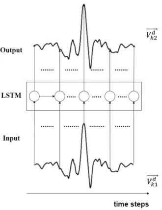
*', respectively. Take the training of a descending dataset as an example, the first data vector 𝑉;;;;;;⃗ _*!+ in 𝐺_*!+ _{is the input of the LSTM and the second data vector}_𝑉

*(+

;;;;;;⃗ is the target of the LSTM. Figure 6 shows the training of the LSTM predictor.

(11)

Figure 7 shows an example of the pre-trained LSTM predictor. A data vector is first selected from the granular wavetable. Then, the predictor uses the current data vector to predict the next one. There are five subsequent data vectors generated from the predictor. As one can see, there are significant differences between the first 4 data vectors and the last two. Hence, we will use a new data vector from the granular wavetable for the replacement. In the future, it is desired to improve the predictor so that one doesn’t have to perform the replacement so frequently.

(12)

3.2.2 The Granular Wavetable

Under some circumstances, it is desired not to use the LSTM predictor to maintain the sound quality. From the datasets obtained in the analysis stage, a granular wavetable is obtained by using the data for each dataset. In order to reduce to the sizes of the granular wavetables, K-Means clustering algorithm is applied to all the datasets independently. After the clustering, only the centers of the clusters are preserved. The conditions to use the granular wavetable are described in the next subsection. Whenever a new data vector from the granular wavetable is required, the cluster center causing least amount of difference between the current waveform is selected.

3.3 The Synthesis Stage

The synthesis system is shown in Figure 8. Our synthesis system is based on source-filter model. The source is an impulse train and the interval between two impulses depends on the required instant pitch of sound. The filter coefficients are generated by the pre-trained LSTM predictor or the granular wavetable. In the beginning, an initial data vector is selected from the granular wavetable as the initial system output. The LSTM predictor will generate the filter coefficients based on the current and previous output waveform. When certain conditions are met, a new data vector will be selected again from the granular wavetable and the LSTM prediction operation resumes. The conditions to switch to the granular wavetable includes: it is required to switch from descending/ascending to ascending/descending; it is required to switch from a part to the next part, for example, from D to S; the difference between the LSTM prediction result and the current data vector is greater than a preset

(13)

threshold. A flowchart of the substitution algorithm to handle the above conditions is shown in Fig 9. At last, the resultant output waveform is multiplied by the ADSR envelope to generate the final synthesized sound.

4. Experiment and Result 4.1 Experiment Setup

The violin recording in the RWC music database is chosen [32]. The file “153VNNVM.wav” in the RWC music database consists of notes from G3 to E7, recorded at mono 16-bit, 44.1KHz. We use C#4 note as our analysis target. Instead of five parts, it is split into three parts, A, S, R, which are enough for this note. The training parameters of all the LSTM predictors are the same. The dimension of the input data vector is 1, the time step is 201 and the output data vector size is same as the input size. The initial learning rate is set as 0.001 and is decremented by 10% every 30 epochs. The number of LSTM layers is 2 and the number of hidden units is 64. The hidden units are connected to a linear output layer. The dropout rate is set

(14)

to 0.5. Finally, mean-square-error (MSE) is used as the loss function. The training always converges within 200 epochs.

4.2 Synthesis Result

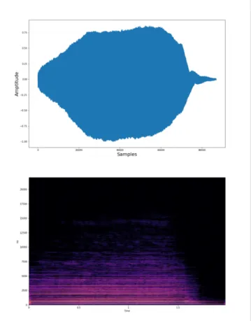
Figure 10 shows a recording of a non-vibrato violin note C#4 and its spectrogram. Figure 11 shows the re-synthesis result. The next experiment is to use the LSTM predictor and the granular wavetable of the C#4 note to synthesize notes of various pitches. Figure 12 shows a synthesized result of non-vibrato G4 note and its spectrogram. Vibrato is essential to violin playing. Figure 13 shows the synthesis result of a vibrato G4 note and its spectrogram. The sound sample can be found online: https://drive.google.com/drive/folders/1kFKL4E0R-S1Bj27kMH-9MB9vEy0_6xX3?usp=sharing

(15)

5. Conclusion and Future Works

A new analysis/training/synthesis method for bowed-string instruments combined with a source filter model and machine learning technologies is presented in this paper. Synthesis of violin sounds is difficult because of its time-varying characteristics due to the various playing techniques and ever-changing dynamics of bow-string interaction. In the analysis stage, recorded bowed-string instrument

(16)

tones are separated into several datasets dependent on the ADSR locations and the ascending/descending statuses of segments of the signals. These datasets are used in two different ways in the training stage. A granular wavetable is used as the initial excitation when the synthesis faces various conditions stated in the paper. A recurrent neural network (RNN) predictor is used to update the filter coefficients of the synthesis model. The training uses popular K-means and LSTM models. The synthesis uses very simple source filter model with the coefficients constantly updated by the proposed algorithm. Though it takes lots of computation in the training stage, the synthesis is simple and efficient. In this paper, a C#4 violin tone in the popular RWC dataset [32] is used to synthesize violin tones of different pitches. Vibrato, tremolo and other processing cab be done efficiently, too. The re-synthesis results sound very close to the recorded tone, too. In the future, more processing will be developed for the various violin playing techniques. It is expected that this method can be applied to wind instruments, too.

Reference

[1] Andresen, U., “A new way in sound synthesis,” in Audio Engineering Society Convention 62, Audio Engineering Society, 1979.

[2] Chowning, J. M., “The synthesis of complex audio spectra by means of frequency modulation,” Journal of the audio engineering society, 21(7), pp. 526–534, 1973. [3] Smith, J. O., “Physical modeling synthesis update,” Computer Music Journal, 20(2), pp. 44–56, 1996.

[4] Smith, J. O., “Physical modeling using digital waveguides,” Computer music journal, 16(4), pp. 74–91, 1992.

[5] Serra, X., “A system for sound analysis/transformation/synthesis based on a deterministic plus stochastic decomposition,” 1989.

[6] Serra, X. et al., “Musical sound modeling with sinusoids plus noise,” Musical signal processing, pp. 91–122, 1997.

[7] Välimäki, V., Pakarinen, J., Erkut, C., and Karjalainen, M., “Discrete-time

modelling of musical instruments,”Reports on progress in physics, 69(1), p. 1, 2005. [8] Välimäki, V., Huopaniemi, J., Karjalainen, M., and Jánosy, Z., “Physical

modeling of plucked string instruments with application to real-time sound synthesis,” in Audio Engineering Society Convention 98, Audio Engineering Society, 1995. [9] Välimäki, V., “Physics-based modeling of musical instruments,” Acta Acustica united with Acustica, 90(4), pp. 611–617, 2004.

(17)

[10] Penttinen, H., Pakarinen, J., Välimäki, V., Laurson, M., Li, H., and Leman, M., “Model-based sound synthesis of the guqin,” The Journal of the Acoustical Society of America, 120(6), pp. 4052– 4063, 2006.

[11] Smith, J., “Acoustic modeling using digital waveguides,” Musical Signal Processing, 7, pp. 221–264, 1997.

[12] Smith, J. O., “Principles of digital waveguide models of musical instruments,” in Applications of digital signal processing to audio and acoustics, pp. 417–466,

Springer, 2002.

[13] Smith, J. O., Music applications of digital waveguides, 39, CCRMA, Dept. of Music, Stanford University, 1987.

[14] Atal, B., “High-quality speech at low bit rates: Multi-pulse and stochastically excited linear predictive coders,” in ICASSP’86. IEEE International Conference on Acoustics, Speech, and Signal Processing, volume 11, pp. 1681–1684, IEEE, 1986. [15] Moorer, J. A., “Signal processing aspects of computer music: A survey,” Proceedings of the IEEE, 65(8), pp. 1108–1137, 1977.

[16] Bass, S. and Goeddel, T., “The efficient digital implementation of subtractive music synthesis,” IEEE Micro, (3), pp. 24–37, 1981.

[17] Klapuri, A., “Analysis of musical instrument sounds by source-filter-decay model,” in 2007 IEEE International Conference on Acoustics, Speech and Signal Processing-ICASSP’07, volume 1, pp. I–53, IEEE, 2007.

[18] Migneco, R. V. and Kim, Y. E., “Excitation modeling and synthesis for plucked guitar tones,” in 2011 IEEE Workshop on Applications of Signal Processing to Audio and Acoustics (WASPAA), pp. 193–196, IEEE, 2011.

[19] Hahn, H., Röbel, A., Burred, J. J., and Weinzierl, S., “Source-filter model for quasi-harmonic instruments,” 2010.

[20] Li, P. C., Chang, W. C., Wang, T. M., Kuo, Y. H., and Su, W.-Y., “Source filter model for expressive Gu-Qin synthesis and its iOS app,” in 16th International

Conference on Digital Audio Effects, DAFx 2013, National University of Ireland, 2013.

[21] Cochocki, A. and Unbehauen, R., Neural networks for optimization and signal processing, John Wiley & Sons, Inc., 1993.

[22] Drioli, C. and Rocchesso, D., “A generalized musical-tone generator with application to sound compression and synthesis,” in 1997 IEEE International Conference on Acoustics, Speech, and Signal Processing, volume 1, pp. 431–434, IEEE, 1997.

[23] Su, A. W. and San-Fu, L., “Synthesis of pluckedstring tones by physical

modeling with recurrent neural networks,” in Proceedings of First Signal Processing Society Workshop on Multimedia Signal Processing, pp. 71–76, IEEE, 1997.

(18)

[24] Liang, S.-F., Su, A. W., and Lin, C.-T., “Model-based synthesis of plucked string instruments by using a class of scattering recurrent networks,” IEEE transactions on neural networks, 11(1), pp. 171–185, 2000.

[25] Ystad, S., “Sound modeling applied to flute sounds,” Journal of the Audio Engineering Society, 48(9), pp. 810–825, 2000.

[26] Pekonen, J., “Computationally efficient music synthesis–methods and sound design,” Master of Science (Technology) thesis, TKK Helsinki University of Technology, Espoo, Finland, 2007.

[27] Gers, F. A., Eck, D., and Schmidhuber, J., “Applying LSTM to time series predictable through time-window approaches,” in Neural Nets WIRN Vietri-01, pp. 193–200, Springer, 2002.

[28] Filonov, P., Lavrentyev, A., and Vorontsov, A., “Multivariate industrial time series with cyberattack simulation: Fault detection using an lstm-based predictive data model,” arXiv preprint arXiv:1612.06676, 2016.

[29] Hochreiter, S. and Schmidhuber, J., “Long short-term memory,” Neural computation, 9(8), pp. 1735–1780, 1997.

[30] Graves, A., Mohamed, A.-r., and Hinton, G., “Speech recognition with deep recurrent neural networks,” in 2013 IEEE international conference on acoustics, speech and signal processing, pp. 6645–6649, IEEE, 2013.

[31] Rashid, K. M. and Louis, J., “Times-series data augmentation and deep learning for construction equipment activity recognition,” Advanced Engineering Informatics, 42, p. 100944, 2019.

[32] Goto, M., Hashiguchi, H., Nishimura, T., and Oka, R., “RWC music database: Music genre database and musical instrument sound database,” 2003.

(19)

科技部補助專題研究計畫出席國際學術會議心得報告

日期：109 年 6 月 15 日

一、參加會議經過

這次因為新冠肺炎疫情的關係，本來要前往現場參加的會議，在詢問過主辦單

位後，同意以線上直播的方式進行報告。殊不知，到了會議前一個禮拜，義大利開

始封城，主辦方告知，他們除了藥局以及超商外，其餘場所皆無法進入，（包括機

構及會場），所有的報告都變成線上預錄或直播的形式了。我先預錄好影片後，待

到會議當天，再由主辦單位統整其他與會者的問題，做統一的答覆，雖然很可惜沒

有辦法親自前往義大利參加會議，卻也是個難得的經驗。

二、與會心得

很感謝這次的計畫能讓我參加這個會議，雖然疫情的關係沒有辦法到現場，但

是從準備的過程中，我也學到了很多，不管是論文的撰寫修改，或是事情的準備，

都從中獲益良多。另外，我也看到了其他投稿的論文，無論是從工程領域或是教育

方面切入，對音樂進行分析研究，都相當地有趣。

三、發表論文全文或摘要

ABSTRACT

計畫編號

MOST 106－2221－E－006－223－MY3

計畫名稱