Abstract—In this paper, the contact force control is investigated for a constrained one-link flexible arm. A minimum phase transfer function involving transcendental functions is obtained by using the method of output redefinition. Then, an integral controller is designed to accomplish the regulation of the contact force. With the infinite product representations of transcendental functions, exact solutions of the noncollocated infinite-dimensional closed-loop force control system are obtained. Numerical simulations are provided to verify the effectiveness of the proposed approach.
I. INTRODUCTION
Force control of constrained flexible manipulators has been receiving a great attention in recent years. Related applications include space robots for satellite capturing and large space structure construction, and also light weight industrial robots for assembly, deburring and grinding tasks, etc. However, it is quite difficult to design such a force controller because of the distributed parameter nature, noncollocation of torque actuation and contact force sensing in the flexible arms.
A large number of approaches regarding various types of constrained flexible manipulators have been published in the literature since 1988 [1-8]. For instance, Chiou and Shahinpoor [1-2] began a research in a single-link and a two-link constrained flexible manipulators by using the finite-dimensional approximate models. The outcome revealed that the link flexibility is the main source of dynamic instability of the force controlled systems. Later, in [3], Li indicated that an inherent limitation on the achievable bandwidth of force control occurs due to the presence of infinitely many non-minimum phase zeros. It is known that the flexible arm is inherently infinite- dimensional system in nature. As a result, the design of the finite-dimensional controller for the constrained one-link flexible arm may become more complicated using the distributed parameter model. Obviously, this phenomenon posted a difficulty for such a model to be realized.
Somehow, the problem was overcome using the Lyapunov method by Morita et al. [4] and Endo et al. [5]. The asymptotic stability of the closed-loop system was also achieved. But the proposed method was found only in a sufficient condition for the constrained one-link flexible manipulator system. Recently, Bazaei and Moallem [6]
proposed a distributed parameter model for a constrained flexible beam actuated at the hub, achieving the maximum control bandwidth. Bazaei and Moallem [7] extended their work to improve force control bandwidth of the constrained one-link arm through output redefinition. Unfortunately,
Liang-Yih Liu is with the Chienkuo Technology University, Taiwan.
phone: 886-4-7111111; fax: 886-4-7111164; e-mail: lliu @ cc.ctu.edu.tw . Hsiung-Cheng Lin is with the National Chin-Yi University of Technology, Taiwan. e-mail: [email protected].
the suppression of high frequency modes may pay a high cost because of degrading the performance attainable.
To overcome the limitations of above papers, the constrained single-link flexible manipulator studied by [8]
with the linear distributed parameter model was used as a starting point. In this research is to develop a perfect asymptotic tracking of a desired contact force trajectory can be achieved using the proposed linear distributed parameter model in the constrained one-link flexible arm.
Section II describes the dynamic model that mainly contains the motion equations and non-minimum phase transfer function. In Section III the proposed controller design is provided. The integral control of the parallel compensated system. The numerical simulation results are presented in Section IV. Section V gives the conclusions.
II. DYNAMIC MODEL
A. Derivation of Motion Equations
The constrained one-link flexible arm depicted in Fig. 1 is a uniform, homogeneous, and Euler-Bernoulli beam, with length , mass per unit length , and flexural rigidity
EI
. The hub is modeled by a single-mass moment of inertia I , where the driven torqueh (t)is applied. The end-effector has a concentrated mass mp, and the contact force exerted by the smooth rigid constraint surface is (t). Reasonably, the arm is assumed moving in a horizontal plane so that the gravity can be ignored. Let the X-axis be a fixed frame and x-axis be a floating frame, both coinciding with the neutral axis of the beam. The hub angular displacement(t)is defined as the counterclockwise rotation of the x-axis. Let) , (x t
v be the small transverse deflection of the neutral axis in the beam. Due to small transverse deflection, the axial displacement u(x,t) caused by bending foreshortening is negligible. Since v(t)v(,t) is assumed small, (t) must also be small. Therefore, the constraint equation for the end-effector can be expressed as
v (t),
(t)
v (t)
(t)0
(1)The kinetic energy
T
and potential energy U are given by
0
2 ( ) ( , ) 2
2 ) 1 2 (
1I t x t v x t dx
T h
(2) Liang-Yih Liu, Hsiung-Cheng Lin
New output control design for a constrained flexible robot
dx t x EIv U
0 xx2 ( , ) 2
1 (3)
where the dot indicates differentiation with respect to the time t, and the subscript
x
denotes partial differentiation with respect tox
.
Ih
( )t
( )t v x t( , )
mp
( )t
X
x
x u(x,t)
Fig. 1. Schematic of a constrained flexible arm.
Note that the kinetic energy of the end-effector mp is neglected since u ( ,t) is negligible. The virtual work by the external torque is given by
W (4)
Apply the extended Hamilton’s principle and the Lagrange multiplier method, i.e.,
0
2 1
tt TU W dt (5) The following integral-partial differential equations from the motion and boundary conditions can be obtained as follows.
( ) ( ) ( , ) ( ) ( )
0 x x t v x t dx t t
t
Ih
x(t)v(x,t)
EIvxxx(0,t) 0 (6) (7)
0 ) , 0 ( t
v (8)
0 ) , 0 ( t
vx (9)
0 ) , ( t
vxx (10)
) ( ) ,
( t λ t
EIvxxx (11)
The (6) can be rewritten as (12) by substituting (7) and (11), performing integration using (10).
) ( ) , 0 ( )
(t EIv t τ t θ
Ih xx (12)
The joint angular acceleration θ(t) can be measured [9-10]. Consequently, a new joint input variable
) (t
u can be expressed as
) ( )
( )
(t t I t
u h (13) Then, (12) is simplified as
) ( ) , 0
( t u t v
EI xx (14)
A. Non-Minimum Phase Transfer Function
The transfer function can be derived by taking the Laplace transform of (1) and (7)-(13) assuming zero initial conditions. Let
s
be the Laplace transform variable, and define the dimensionless parameters , ,
, and sˆ as2 4 2
4 s ˆs
EI
, 3
ρ
ε Ih (15)
Then, (7) can be expressed as
) ( )
( )
( 4
4 4
4
v x x
x
v (16)
The solution is obtained as
x x C
x C
x C
x C
x v
sin
sinh cos
cosh )
, (
4
3 2
1
(17) where Ci() , i 1, 2,3, 4 is an unknown parameter. The substitution of (17) into (1), (8)-(13), involving C , 1 C , 2 C , 3 C , 4 , ,
andu
. The C , 2 C , 3 C , 4 , ,
andu
can be solved in terms of C , shown as follows.11
2 C
C , 3 sinh 1
cosh C
C
, 4 sin 1
cos C
C
(18)
sinh sin
sinh cos sin ) cosh
(ˆ 1
C
s (19)
sinh sin
sinh ) sin
(ˆ 3
3 1
C EI
s (20)
sin sinh
sin cosh sinh
2 cos ˆ)
( 1 22 3
EI C s
(21)
2 2
2 1
ˆ)
(
EI C s
u (22)
Using (17), one further obtains
2 2
2 1
ˆ) , 0
(
C s
vxx (23)
With the infinite product of transcendental functions given in the Appendix, it verifies that
1 2
2
1 2
2
3
1 ˆ 1 ˆ 1
) cos sinh sin
(cosh sin
sinh 2
sin sinh ˆ)
( ˆ) ) ( (ˆ
n n
n zn
s s s s s G
(24)
1 4 4
2
1 2
2
1 ˆ 1 ˆ 1
sin sinh
sin sinh 2 ˆ) (
ˆ) ) ( (ˆ
n
n zn
u
n s s s
u s s G
(25)
1 4 4
2
1 2
2 3
1 ˆ 1 ˆ
sin sinh 2
) cos sinh sin
(cosh sin
sinh 2
ˆ) (
ˆ) ) ( (ˆ
n
n n
u
n s s s u s s G
(26)
1 4 4
2
1 2
2
1 ˆ 1 ˆ
3 ˆ) (
ˆ) ) ( (ˆ
n
n n
u
n s s EI
s u s s G
(27)
EI s
u s s v
Gv u xx
xx
1 ˆ)
( ˆ) , 0 ) (
(ˆ (28)
where zn and n are defined, as shown in the Appendix. The numerical values of n() can be computed using n n2, where n(),
, 2 ,
1
n is the real positive roots of the denominator of (24), namely
0 ) cos sinh sin
(cosh sin
sinh
2 3
(29) The values obtained by selected n are listed in Table I.
III. CONTROLLER DESIGN L
A. Achieving minimum phase passivity using Output Redefinition
For non-minimum phase systems, it is known that the asymptotic tracking of output trajectories with internal stability cannot be achieved accurately. Based on the control theory concept, this problem can be resolved replacing the right half-plane zeros by the left half-plane zeros. Consequently, define a new virtual contact force
) , ( kt
f such that
sin sinh
) cos cosh 1 ( ) 1 ( ) sinh (sin
2
ˆ) (
) ˆ, ) ( ˆ, (
k k
s u
k s k f
s Gfu
(30) where k is a real constant whose permissible values will be determined to satisfy the minimum phase condition.
Now, the numerator of Gfu( ksˆ, ) is written as
) cos cosh 1 ( ) 1 ( ) sinh (sin
) ,
( k k k
N
(31) Then, using (15) for the zeros of Gfu( ksˆ, ) are given by the roots of
1 1 ˆ
1 ˆ
1
1 2
2
1 2
2
m pm
n zn
ω s ω s k
k (32)
where A1 and A4 from the Appendix have been used in deriving (32). Note thatpmare the well-known clamped- free bending vibration modes. The lowest 6 modes of
zn and pm are listed in the Appendix. The root locus of (32) for k 1 is shown in Fig. 2 based on a 6 pole-zero pair approximation. The approximate breakaway points on the imaginary sˆ -axis are
, 10 . 92 , 20 .
12 j j
260.66j corresponding
to k 0.759, 0.918, 0.984, respectively. Note that the breakaway points on the imaginary sˆ -axis actually corresponds to the real positive double roots of
, 0 ) , ( k
N or equivalently,
) sin (sinh
1 1 1
cos
cosh
k
k
(33) Further, the asymptotic behavior of (33) is governed by
k k
1
cos
(34)
It is easy to verify from the numerical solutions of (33) and simple graph of (34) that (i) the smallest real positive double roots 3.483 (sˆ 12.132j) occur when
, 758 .
0
k (ii) a larger value of real positive double roots occur at a larger value of k , and (iii) there are no
real positive double roots for
. 758 .
0
k Therefore it is impossible to have any breakaway
TABLE I
VALUESOFROOTSOFASSOCIATEDTRANSCENDENTALEQUATIONS
n n(k 0.7) n ωθn(ε 3.387102)
8472
.
2 4.9002 2.6862
0822
.
4 7.7252 4.4102
1452
.
8 11.0862 7.1562
7772
.
10 14.0662 10.2382
3012
.
14 17.3362 13.3642
(nodd) (n even)
2
2) ( 1 3 ) 7 2 ( 1
n n
2
2) ( 1 3 ) 7 2 ( 1
n n
2
2) ( 1 ) 1 2 ( 1
n n
2
2) ( 1 ) 1 2 ( 1
n n
2
3
)3
4 ( 3
5 . ) 29
4 ( 3
π n
π n
1 2
3
4
5n
(nodd) (n even) …
.….
….
….
point on the imaginary sˆ -axis for k 0.758. We conclude that, with the previously defined new input and output, the constrained one-link flexible manipulator is minimum phase iff k 0.758. We emphasize here that this necessary and sufficient condition is obtained via the numerical solution of the exact transcendental equation N(,k)0, not by the finite-dimensional approximation of the root locus.
One can write
1 2
ˆ2
1 2
) cos cosh 1 ( ) 1 ( ) sinh (sin
n n
s
k k
(35) The numerical values can be computed using
n2
n
, where n(k), n 1,2, is the real positive roots of the numerator of (35). Selected n
values are listed in Table I. Thus, one deduces a minimum phase stable transfer function as
1 4 4
2
1 2
2
1 ˆ 1 ˆ ) 1
ˆ, (
n
n n
u f
n s s k
s G
(36)
Note that the above redefinition of output is equivalent to the parallel compensation as shown in Fig. 3(a). The parallel compensator T(sˆ,k) has the form
-300 -200 -100 0 100 200 300
0 40 80 120
Im (s)
Re ( )s
k=0 0.7589 k=0 k=0
0.9176
k=0
1 1 1
1 1
1 1 1
Fig. 2. Root locus of (32) for k1 using 6 pole-zero pair approximation.
1 4 4
2
1 2
2
2
ˆ ˆ 1
ˆ ˆ 1 1 ˆ
ˆ 120
) 1 ( 11
sinh sin
) sinh (sin
) cos cosh 1 ( )2 1 ( ) ˆ, (
n
n n
n s s
s s s
k s k k
s T
(37) where n n2 and n(k), n1,2 is the real positive roots of the equation
0 ) sinh (sin
) cos cosh 1
(
(38)
Table I shows the outcome by computing the selected
n
values.
B. Integral Control
In what follows, only a simple feedforward integral controller will be considered for the regulation of the contact force λ(t). The control structure, shown in Fig.
3, is to find λ(t) that can asymptotically track a desired
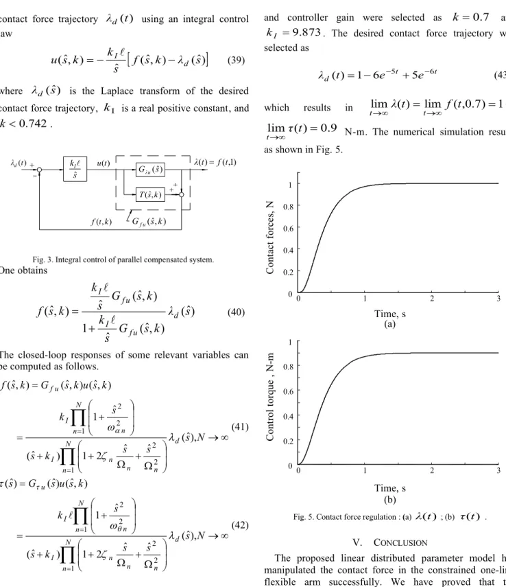
contact force trajectory λd(t) using an integral control law
(ˆ, ) (ˆ)
) ˆ ˆ,
( f s k λ s
s k k
s
u I d (39)
where λd(sˆ) is the Laplace transform of the desired contact force trajectory, k is a real positive constant, andI
742 .
0
k .
Gλu(sˆ)
) ˆ, ( ks T
) , ˆ ( ks Gfu ) , ( kt f )
(t
λd u(t)
s kI ˆ
λ(t)f(t,1)
Fig. 3. Integral control of parallel compensated system.
One obtains
ˆ ) ( ) ˆ , ˆ (
1
) ˆ , ˆ (
) ˆ ,
( λ s
k s s G
k
k s s G
k k s
f
du I f
u I f
(40)The closed-loop responses of some relevant variables can be computed as follows.
s N
s k s
s k s
k s u k s G k s f
N d
n n n n
I N
n n
I u f
ˆ), ˆ (
2 ˆ 1 ˆ )
(
1 ˆ ) ˆ, ( ) ˆ, ( )
ˆ, (
1 2
2
1 2
2
(41)
s N
s k s
s k s
k s u s G s
N d
n n n n
I N
n n
I u
ˆ), ˆ (
2 ˆ 1 ˆ )
(
1 ˆ ) ˆ, ( ˆ) ( ˆ)
(
1 2
2
1 2
2
(42)
IV. SIMULATION
The effectiveness of the proposed control approach is evaluated here through numerical simulation using the parameters of an experimental apparatus described in [11].
These parameters are : ρ0.405 kg/m, 1011
06 .
2
E N/m2, 0.9m,
10 11
41 .
1
I m4, Ih 0.01 kgm2 ( 10 2
387 .
3
ε ). The virtual contact force parameter
and controller gain were selected as k0.7 and 873
.
9
kI . The desired contact force trajectory was selected as
t
d t e t e
λ ( )16 5 5 6 (43)
which results in lim ( ) lim ( ,0.7)1
λ t f t
t
t N,
9 . 0 ) (
lim
τ t
t N-m. The numerical simulation results as shown in Fig. 5.
Time, s (a)
Time, s (b)
Fig. 5. Contact force regulation : (a)λ(t) ; (b) τ(t) .
V. CONCLUSION
The proposed linear distributed parameter model has manipulated the contact force in the constrained one-link flexible arm successfully. We have proved that the noncollocated system is a non-minimum phase when the joint torque is used as the input to generate the tip contact force as the output. A minimum phase transfer function can be therefore obtained by generating a new input and output via the feedback of joint angular acceleration. Numerical performance results are provided to verify the effectiveness of the proposed approach in term of fast, stable and robust performance.
0 1 2 3
0 0.2 0.4 0.6 0.8 1
0 1 2 3
0 0.2 0.4 0.6 0.8 1
Contact forces, NControl torque , N-m
APPENDIX
In accordance with the context of this paper, sˆ2 4 is used whenever it is appropriate.
A1.
1 2
ˆ2
1 2
sinh sin
n zn
s
A2.
1 4 4
2 ˆ2
1 sinh
sin
n n
s
A3.
1 2
3 ˆ2
3 1 sinh 2 cos sin
cosh
n n
s
A4.
1 2
ˆ2
1 2 cos cosh 1
n pn
s
Note that the asymptotic expressions are found very accurate (to three decimal places) since n5.
REFERENCES
[1] B. C. Chiou and M. Shahinpoor, “Dynamic stability analysis of a one-link force-controlled flexible manipulator,” Journal of Robotic Systems, vol. 5, no. 5, pp. 443-451, Oct. 1988.
[2] B. C. Chiou and M. Shahinpoor, “Dynamic stability analysis of a two-link force-controlled flexible manipulator,” ASME Journal of Dynamic Systems, Measurement, and Control, vol. 112, no. 4, pp.
661-666, Dec. 1990.
[3] D. Li, “Tip-contact Force control of one-link flexible manipulator: an inherent performance limitation,” Proceedings of 1990 American Control Conference, San Diego, CA., May 1990, pp. 697-701.
[4] Y. Morita, F. Matsuno, M. Ikeda, H. Ukai and H. Kando,
“Experimental study on PDS force control of a flexible arm considering bending and torsional deformation,” 7th International Workshop on Advanced Motion Control, Maribor, Slovenia, July 2002, pp. 408-413.
[5] T. Endo and F. Matsuno, “Dynamics based force control of one-link flexible arm,” SICE 2004 Annual Conference, Sapporo, Aug. 2004, pp. 2736-2741.
[6] A. Bazaei and M. Moallem, “Force transmission through a structurally flexible beam: dynamic modeling and feedback control,” IEEE Transactions on Control Systems Technology, vol. 17, no. 6, pp. 1245- 1256, Nov. 2009.
[7] A. Bazaei and M. Moallem, “Improving force control bandwidth of flexible-link arms through output redefinition,” IEEE/ASME Transactions on Mechatronics, vol. 16, no. 2, pp. 380-386, Apr. 2011.
[8] L. Y. Liu and K. Yuan, “Force control of a constraint one-link flexible arm: a distributed parameter modeling approach,” Journal of Chinese Institute of Engineers, vol. 6, no. 4, pp. 443-454, June 2003.
[9] H. Motoaki and M. Toshiyuki, “Vibration control of flexible arm by multiple observer structure,” Electrical Engineering in Japan , Vol. 154, No. 2, pp. 68-75, 2006.
[10] Q. Zhicheng, “Acceleration Sensor Based Vibration Control for Flexible Robot by Using PPF Algorithm,” 2007 IEEE International Conference on Control and Automation, Guangzhou, CHINA, May 30-June 1 2007, pp. 1335-1339.
[11] F. Matsuno and S. Kasai, “Modeling and robust force control of constrained one-link flexible arms,” Journal of Robotic Systems, vol.
15, no. 8, pp. 447-464, Aug. 1998.