Modeling and Control of Household-Size Vertical Axis Wind Turbine and Electric Power Generation System

Modeling and control of household-size vertical axis wind turbine and electric power generation system

Harki Apri Yanto

¹

Chun-Ta Lin

²

Jonq-Chin Hwang

²

Sheam-Chyun Lin

¹

1

Department of Mechanical Engineering

2

Department of Electrical Engineering

National Taiwan University of Science and Technology Taipei, Taiwan

Abstract— This paper discusses the design of a low tip-speed ratio, drag type vertical axis wind turbine which is incorporated with permanent magnet synchronous generator with maximum power point tracking (MPPT) strategy of control system to acquire the optimal performance. By using two dimensional large eddy simulations (LES) method as fluid dynamic model, the calculated power coefficient for this multi-blade vertical axis wind turbine may reach 0.34 at tip speed ratio (TSR) ranging from 0.8 to 1.0. Also, with the aids of simulation results, a direct coupled permanent magnet synchronous generator with 64-poles is designed and fabricated to generate 1.5 kW rated power at 90 rpm in 12 m/s wind speed. By changing the shape of magnet and applying approximate-skew method as stepped magnet configuration, the cogging torque and noise level of generator can be minimized. Moreover, MPPT control system with low current harmonic distortion level is designed to transfer energy into power grid with estimated 92% of power efficiency.

Consequently, by eliminating gearbox system, low start-up wind speed, low current harmonic distortion and low cogging torque, the proposed of low acoustic/noise level wind turbine generator system can be applied for urban-environmental usage.

Keywords - Vertical-axis Wind Turbine(VAWT); Permanent Magnet Synchronous Generator(PMSG); Maximum Power Point Tracking(MPPT)

I. I NTRODUCTION

Recently, many countries attempt to develop the household- scale vertical axis wind turbines as a green energy industry.

Several researches are conducted on the wind turbine generator system (WTGS), such as aerodynamic characteristic for lift type and drag-type vertical axis wind turbines (VAWT) [1]-[7].

Since most VAWT tend to yield negative torque when the blade is opposing to the wind direction, the aerodynamic characteristic of multi-blade as novel design of vertical axis wind turbine [8] are studied. The design purpose of this novel drag-type of VAWT is to eliminate the negative torque angle when the blade rotates.

For the previous electrical system research, coreless axial- flux type permanent magnet generator [9] has been used to minimize the aerodynamic start-up torque by reducing the cogging torque of generator; however, it also demonstrated a worse performance characteristic compared to the permanent magnet generator.

Therefore, a combine system between low wind speed start- up turbine, radial-flux type permanent magnet synchronous generator (PMSG) [10], and grid-connected control system design is purposed here. By using computational fluid dynamic (CFD) and finite element analysis (FEA), the performance of WTGS integrated with grid-connected system need to be studied. The illustrated of system diagram can be seen on Fig.

1.

Ls R_s eaG+

− iaG

Ls Rs ebG+

− i_bG

Ls R_s ecG+

− i_cG

iC vdc Cdc

+

− 1

Ta⁺ Tb1⁺ Tc1⁺

1 Ta⁻ Tb⁻1 Tc1⁻

idco idci

a b

c

1 Tr⁺ Tr⁺2

1 Tr⁻ Tr⁻2

r1

r2 vrf Lf

Cf

irf L_sc R_sc

er ir

VAWT

ωm

vwind

Wind Turbine Multi-blade vertical axis wind turbine T ype Drag Type

Dimension D= 4m, H= 2.1m

Ge nerator Permane nt Magne t Synchronous Ge nerator T ype 64 poles- 60 slot radial flux Control System AC/DC/AC MPPT strategy Spe e d control Specification

PMSG

110V grid

Fig. 1. The Overall System Diagram II. W IND T URBINE D ESIGN AND A NALYSIS

The multi-blade, drag-type VAWT is a modified version of

windmill type VAWT. This multi-blade VAWT consists of 8

sets of blades with crossed configuration. A set of blades

contains two identical blades installed oppositely with 90 º

difference from blade’s axis. With this 90º difference, one

blade faces the wind direction while other blade lays along the

wind direction for each level. When the wind turbine rotates

around the vertical axis, the facing-wind position’s blade will

be pushed by the thrust force in the counter clockwise direction

and the leaning-wind position’s blade is pulled with a small

negative drag force. Until a certain angle of rotor rotation, the

thrust force will be depleted due to rotation angle of the wind

turbine. When the moment of thrust force becomes lower

compared to the moment generated by gravity of the blade, the

blade will automatically flap into the lay condition. Due to this

self-flapping motion, each blade will flap 90°from facing the wind condition into laying position by the balancing action from moment created by gravity of the opposite blade. This flap motion will reduce the negative torque for downwind blade. Fig. 2 illustrates the blades’ movements and the torque output of each pair of blade under various rotation angles.

-1 -0.5 0 0.5 1

0 60 120 180 240

θ(degree)

Torque Coefficient

Fig. 2. Torque Distribution from Various Positions

The drag forces created by the rotor blades eventually provide the thrust force and torque to the WTGS. A 2D CFD analysis is performed by using the commercial code Fluent to calculate the aerodynamic properties, such as coefficient of moment (C

m

), tip-speed ratio (TSR), and power estimation. The simulation model is plotted in Fig.3.

By using Large Eddy Simulation method, each blade’s coefficient of moment can be accurately estimated for each rotation angle as shown in Fig. 2. By averaging the C

m

for all rotation angles with a minimum 4 rotation cycles as the database, the coefficient of torque (C

t

) for one operation condition can be obtained. With knowing the C

t

for every operation condition, it follows that the coefficient of power (C

p

) for wind turbine can be estimated.

m

t

C

C = ⁽¹⁾

t

p

TSR C

C = . (2)

Wind turbine is simulated under different TSR conditions to evaluate its aerodynamic characteristics. From observing these estimated aerodynamic characteristic, the optimum performance (C

p

= 0.3) for this wind turbine is found at the case of TSR= 0.8 as indicated in Fig. 4(a).

From the flow field analysis at TSR = 0.8 condition, it is obvious that turbulence flow occurs behind the blades. This phenomenon can be seen when the wind turbine rotates around -10º to 40º.Note that the case of 0º represents that the blade position is facing to the wind direction perpendicularly.

Because of separated flow past a flat plat and velocity difference between relative rotor velocity and relative blade tip’s velocity, the turbulence flow is generated behind the blade as plotted in Fig. 5. This turbulence flow results in the low pressure region, which may become resistant either for blade to flap or rotate in vertical axis.

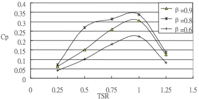
In order to minimize the velocity difference between relative rotor velocity and relative blade tip’s velocity, the blade length ratio (β) is modified for enhancing the wind turbine’s performance. After evaluating different β parameters ( 0.6, 0.8, and 0.9), the corresponding aerodynamic performances are calculated and used to identify the optimized performance. The results of blade length variation are indicated in Fig. 6. Apparently, it is found that the shorter blade length ratio will diminish the turbulence flow behind the blade. In the other hand, reducing the blade area too much may also cause the decreasing of aerodynamic performance of wind turbine.

The case of β=0.8 yields the best choices among all the other cases considered in this study, which generate C

_p

=0.34 at TSR

= 0.96. Consequently, the optimized wind turbine performance can be estimated and indicated in Fig. 4 (b).

Fig. 3. 2D Simulation Model of Multi-Blade VAWT System

Fig. 4. The Aerodynamic Characteristics: (a)Ct and Cp Estimations for Different TSRs. (b) Estimated Wind Turbine Performance

Fig. 5. Turbulence Initiallazation Flow Pattern of a Pair Blade Captured at

the condition of 0˚, TSR= 0.25

Fig. 6. Power Coefficient vs Tip-Speed Ratio for Different Blade Ratios III. G ^ENERATOR D ^{ESIGN AND} A ^NALYSIS

Directly-couple between PMSG and wind turbine, is chosen to reduce transmission loss. By configuring 64-pole, 60-slot permanent-magnet with 1.0667 pole-to-slot ratio, a greater magnetic efficiency and smaller cogging torque can be achieved. After that, optimization process using FEA for shapes of magnet, stator teeth and slot with lower EMF criterion is applied to attain the lower electrical noise and torque ripple level. In the end, concentrated winding configuration is chosen in order to shorten the windings length and lower copper loss.

A. Design of Permanent Magnet Synchronus Generator By substituting magneto-motive force balance equation into demagnetization characteristic equation of NdFeB magnet, it can be illustrated

r g g

m r rm

m

K B l

B B

μ ⁻ l

= + (3)

Where K

r

is the reluctance factor, µ

rm

is the relative permeability of magnet, B

g

is the air-gap flux density, B

r

and B

m

are the residual and operating flux densities, respectively.

By assuming the flux leaving the magnet equals to the flux crossing the air-gap, we have

m m g g

B A = B A (4)

From [10], the permeance coefficient is

0

m m g

c

m g m

B l A

P μ H l A

= − = (5)

Since the ferromagnetic material has very high permeability, its reluctance can be ignored, i.e., K

r

=1. Thus equation (3) becomes:

1 1

m r

rm c

B B

P

= μ +

(6)

The static operation point of permanent magnet can be determined as shown in Fig.7 (a). It is reasonable to assume that the cross-section area of air-gap equals to the cross- sectional area of magnet, i.e., A

g

=A

m.

Also, by substituting equation (4) into (6), the relationship between air-gap flux density and remanence can be written as

1 1

g r g

rm m

B B l

μ l

= +

(7)

Fig. 7(b) demonstrates the relationship between l

m

/l

g

ratio and the B

g

/B

r

ratio. The air-gap flux density becomes saturated when the l

m

/l

g

ratio is bigger than 4, therefore, the magnet length l

m

is selected as four times from air-gap length.

Bm

Br

0Hm 0Hcj μ

μ

B

0H μ μrm

Pc

g r

B B

m g

l l

(a) (b)

Fig. 7. Characteristics of Designed Magnet: (a) Static Operation Point of Permanent Magnet; (b) Air-gap flux density vs Remanence Curve Pole-arc to pole-pitch ratio is useful for choosing the width of magnet [17] that is

- arc

p p pitch

r α

= α (8)

where α

arc

is width angle of single magnet, andα

pitch

is the angle between two magnets. To compare the performance between different r

p-p

, a simple surface-mounted permanent magnet (SPM) design is considered, and r

p-p

is increased from 0.5 to 0.85. From FEA analysis result which is shown on table 2, the pole-arc to pole-pitch ratio is selected as 0.65 to minimize the total harmonic distortion (THD) of back EMF.

The stator tooth width, stator yoke width, and rotor yoke width are adjusted to achieve flux density less than 1.4 T and close to the material saturation point.

TABLE. I. C

OMPARISON BETWEEN DIFFERENT POLE

-

ARC TO POLE

-

PITCH RATIOS

Pole-arc to Pole-pitch

ratio

THD of Air- Gap Flux Density (%)

Back EMF

(V, rms) THD of Back EMF

3rd Harmonic

of Back EMF

(%)

5th Harmonic

of Back EMF

(%)

0.5 25.86 112.21 11.9 12.47 1.25

0.55 20.9 119.73 7.68 8.4 1.47

0.6 16.15 126.59 3.72 4.56 1.5

0.65 13.03 132.7 1.63 0.85 1.27

0.7 11.87 137.96 4.1 2.57 0.92

0.75 13.21 142.25 6.72 5.64 0.46

0.8 15.47 145.44 8.7 8.24 0.04

0.85 20.29 147.64 10.06 10.32 0.49 By applying dovetail type method for magnet to rotor assembly, not only improves the structural strength, it also makes the magnet assembling process become easier. From FEA calculation of magnet shape optimization, a smaller generator size and more efficient magnetic performance can be designed and illustrated in Fig. 8. Fig.8 is a cross section drawing of 64-poles 60-slots generator design.

0 0.05 0.1 0.15 0.2 0.25 0.3 0.35 0.4

0 0.25 0.5 0.75 1 1.25 1.5

TSR Cp

β=0.9

β=0.8

β=0.6

Fig. 8. Cross Section drawing of this 64-poles, 60 slots generator.

B. Finite Element Analysis

Overall finite element simulations are accomplished using Maxwell 2D. The generator’s flux lines distribution shows a uniform and symmetric in no-load condition, as plotted on Fig. 9(a). Fig. 9(b) shows the flux density distribution reaches maximum flux density around 1.34 T which is occurred around stator teeth area. This design condition is near with the 50CS400 saturated point at 1.4 T.

The performance of generator at rated speed is plotted on Fig.

10. Fig.10 (a) and Fig. 10(b) are the phase back-EMF and line back-EMF analysis results while generator rotates at 90 rpm rated speed. With the back-EMF has small harmonic distortion (THD) around 2%, which is illustrated in Fig. 10(c), the generator design performs high controllability and low noise possibility.

In order to identify generator performance, the generator is connected with a wye configuration and coupled with a 30Ω wye-connected resistor for full load simulation. From the full- load simulation, copper-loss and core-loss are computed around 58.4W and 18W, with 95% efficiency estimation.

Applying [18], the rotor-flux λ

_m

′ , d-axis inductance L

d

, and q- axis inductance L can be calculated using equation (9)-(10)

_q

with the result 0.6097 V-s/rad, 15.64 mH and 47.08 mH.

r r

rG m qG s qG

d r

rG dG

v R i

L i

ω λ ω

′ − −

= (9)

r r

dG s dG

q r

rG qG

v R i

L ω i

= + (10)

(a) (b) Fig. 9. Flux Distribution at No-Load Magnetostatic Field Simulation results

：(a) Flux Lines；(b) Magneticstatic Flux Density Profile

C. Cogging Torque Reducion

With the aid from Z. Q. Zhu and D. Howe [17], the optimum ratio of pole-arc to pole-pitch, α

^p

is calculated.

Follows with the ratio of pole-arc to pole-pitch near 0.65, a stepped magnet configuration with approximate skew strategy is applied in this generator. Fig. 11 illustrated the rotor construction with angle of skew θ

skew

=0.1875 ˚ and L

stk

is the stack length of rotor core. The cogging torque output is estimated around 0.35% from rated torque loading.

Fig. 10. Generator Characteristics at No-Load Simulation Results: (a) Phase Back-EMF Waveform Chart, (b)Line Back-EMF Waveform Chart;

(c)Spectrum of Back-EMF Chart

2 Lstk

θskew

2 Lstk

Fig. 11. Stepped Magnet with Approximat Skew Strategy Illustration

IV. W IND T URBINE G ENERATOR S YSTEM C ONTROL

A three phase full-bridge full-controlled rectifier and single

phase grid-connected inverter is proposed for easy house-hold

application. This configuration not only will increase the

power factor to near 1, also may reduce the harmonic level of current input and the electromagnetic noise inside generator.

A. Control strategy of three phase full-bridge full-controlled recitifier

Vector control algorithm is selected for rapid current control response and low current harmonic content.

From voltage equations in the rotor reference frame, the voltage equation u

_qG^r

and u

_dG^r

can be defined as:

r r r

qG s qG q qG

r r r

qG rG d dG qG

u R i L d i

dt

e ω L i v

= +

= − −

(11)

r r r

dG s dG d dG

r r r

dG rG q qG dG

u R i L d i

dt

e ω L i v

= +

= + −

(12)

From equation (11) and (12), u

_qG^r

and u

^r_dG

are linearly dependent with i

_qG^r

and i

_dG^r

. By substituting the voltage compensation technique, the d-axis and q-axis current can be controlled independently. The output of current regulator becomes:

*

(

*

)

r r r

qG qG qG qG

u = G D i − i (13)

*

(

*

)

r r r

dG dG dG dG

u = G ^D i − i (14)

where G

_qG

and G

_dG

are PI controllers, and “ D ” is the multiplying operator. By combining all the equation (from equation 11 to equation 14), the v and

^r_qG^*

v can be derived

_dG^r*

into

* *

r r r r

qG qG rG d dG qG

v = e − ω L i − u ⁽¹⁵⁾

* *

r r r r

dG dG rG q qG dG

v = e + ω L i − u ⁽¹⁶⁾

where e

_qG^r

= ω λ′

_{rG m}

^and e

dG^r

= ⁰ . Fig. 12 illustrated the AC/DC close-loop control strategy, where ˆ θ

_rG

is the estimated rotor position. By receive the current deviation feedback, the control system will control v

^*_aG

, v and

_bG^*

v output. This

^*_cG

method also shows a good controllability for active and reactive power.

+

−

* 0

e

idG= ⁺

− e*

iqG GqG ⁻

− e

vqG + e*

vqs

* e

uqs

− +

ˆrG

θ

*

vas

*

vbs

*

vcs

e

idf e

iqf

ˆrG

θ

iaf

ibf

icf e

rL ifG df

ω

e

vdG + e rL ifG qf

ω

* e

uds v^eds^*

GdG

cos sin

sin cos

rG rG

rG rG

θ θ

θ ⁻ θ

⎡ ⎤

⎢ ⎥

⎣ ⎦

cos sin

sin cos

rG rG

rG rG

θ θ

θ θ

⎡ ⎤

⎢− ⎥

⎣ ⎦

1 1

21 2 2

3 3 3

0 2 2

⎡ − −⎤

⎢ ⎥

⎢ ⎥

⎢ − ⎥

⎢ ⎥

⎣ ⎦

1 0

1 3

2 2

1 3

2 2

⎡ ⎤

⎢ ⎥

⎢ ⎥

⎢− − ⎥

⎢ ⎥

⎢ ⎥

⎢− ⎥

⎢ ⎥

⎣ ⎦

Fig. 12. AC/DC Converter Control Strategy

B. Control strategy of single phase grid-connected inverter A single-phase inverter is proposed for grid-connection, it converts the three phase input into single phase with 60 Hz power. By equation (17), the output voltage of inverter v

_φ

can be acquired,

(

^{1 2}

)

^dc

v

_φ

= s − s v ⁽¹⁷⁾

The state equation of inductor L and DC-link capacitor

_s

C can be expressed in equation below,

dc

12

s s

L d i e R i v

dt

^φ

=

^φ

−

^φ

− (18)

(

^{1 2}

)

dc dc dc

C d v s s i i

dt = −

^φ

− (19)

Fig. 13 is DC/AC control strategy diagram, where sin ˆ

_s

u

_φ

= θ ， e

_φ

= E u

_{m φ}

and i

_φ^*

= I u

_m^* _φ

= I

_m^*

sin θ ˆ

_s

. DC-link voltage is tuned through the control of voltage regulator G

_v

and current regulator G .

_i

2

sr

vdc^∗ +

− vdc

Gv

*

Im

⊗ ur

+

− ir^∗

Gi

− + er

vrs^∗ 1 vdc

+ +

− +

1

1

1

dr^∗

2

dr^∗

− +

− + ir

1

sr

1 2

1 2

vt

Fig. 13. DC/AC Converter Control Strategy

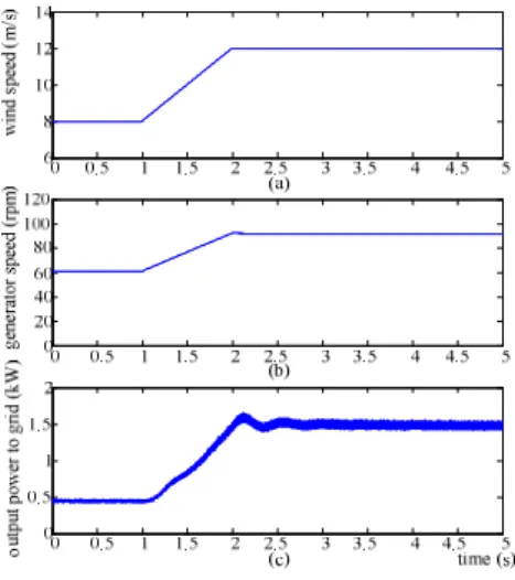
C. Maximum Power Point Tracking Strategy (MPPT)

Speed control method is used in this paper to avoid additional noise generation from MPPT control process. Fig.

14 showed the diagram of MPPT strategy. From aerodynamic simulation, the maximum power coefficient occurs when TSR

= 0.96. The optimized speed can calculate from TSR definition,

_m^{* opt wind}

blade

TSR v

ω = r (20)

where TSR is the TSR with maximum power coefficient

_opt

max

C

p

. Let G

_ωm

as a speed regulator, then

i

_qG^r*

= G

_ωm

D ( ω

_m^*

− ω

_m

) (21) Fig. 14 shows the process how MPPT adjust the generator loading. By tuning the generator’s current output, the generator will be loaded with different torque load.

* r

iqG

G_ωm

vwind

− +

ω

m opt wind

blade

TSR v r

*

ω

m

Fig. 14. MPPT Strategy Block Diagram

V. S YSTEM S IMULATION

The overall system performance is simulated for both the steady-state condition and transient condition in MATLAB/Simulink. From Fig. 15, the steady state simulation at 12 m/s wind speed shows the power factor both input- output are almost near 1, and the current output yields a lower THD. For transient simulation, wind velocity accelerates from 8m/s to 12 m/s is simulated to observe the capturing power ability. From AC/DC/AC grid-connected system with MPPT, it performs well tuned power output. The overall system can correspond to wind velocity change smoothly in rapid time with estimated efficiency around 92%.

Fig. 15. Steady-State Simulation at 12 m/s wind speed: (a) generator back EMF; (b) generator back EMF vs. output current of phase with (THD=2.3%);

(c) grid voltage vs. output current with (THD=1.18%)

Fig. 16. Transient Simulation Result from 8m/s to 12m/s : (a) Wind Speed;

(b) Generator Rotating Speed; (c) Output Power to Grid Chart VI. C ^ONCLUSION

Design and simulation of a small-size WTGS are accomplished in this paper. This complex effort includes the design and aerodynamic simulation of multi-blade VAWT, the design and FEA simulation of radial-flux PSMG, and the analysis of the grid connected AC/DC/AC power converter

with maximum power point tracking strategy. From the simulation result, with blade length ratio β = 0.8, wind turbine may reach maximum Cp ≈ 0.34 at TSR = 0.96. After directly coupled with the 64-poles, 60-slots radial-flux generator and the MPPT grid-connected system, this WTGS system can produce 1.5 kW, 1φ 110 V

_AC

output at wind speed 12 m/s. The estimated efficiency of the overall system may reach 92%. Due to the low acoustic generation, electromagnetic noise, and low start –up wind speed characteristic of this VAWT system, this system is suitable and can be applied as the clear-energy alternative for utility generation.

R EFERENCES

[1] Sandia National Laboratories Staff, “Vertical axis wind turbines the history of the DOE program”., 1999.

[2] Blackwell, B. F., Sullivan, W. N., Reuter, R. C., and Banas, J. F.,

“Engineering development status of the Darrieus Wind Turbine,” J.

Energy, Vol. 1, No. 1, pp, 50-64, Jan. 1977.

[3] Shibuya, S., Fujisawa, N., and Takano, T., “Visualization and PIV measurement of unsteady flow around a Daerrieus wind turbine in dynamic stall,” 7th International Conference on Nulcear Engineering, Tokyo, Japan, pp 19-23, April 1999.

[4] Strickland, J. H., “The Darrieus turbine: a performance prediction model using multiple streamtubes,” SAND75-0431, 1975.

[5] Blackwell, B. F. Sheldahl, R. E., and Feltz, L. V., “Wind tunnel performance data for two- and three-bucket Savonius rotors,” SAND76- 0131, 1977.

[6] Menet, J.L., “A double step Savonius rotor for local production of electricity: a design study,” Renewable Energy, Vol. 29, No. 11, pp.

1843-1862, 2004.

[7] Fujisawa, N., “ On the torque mechanism of Savonoius rotors,” Journal of Wind Engineering Industry Aerodynamic, Vol. 40, No. 2, pp 77-92, 1992.

[8] Huang H. J., “Numerical analysis of the modern vertical axis wind turbine”, master thesis, Dept. Mech Eng., National Taiwan University Science and Technology, 2008.

[9] Wang, R. J, Kamper, M. J., Van der Westhuizen, K., and Gieras, J. F.,

“Optimal design of a coreless stator axial flux permanent magnet generator,” IEEE Transaction on magnetics, Vol. 41, pp.55-64, 2005.

[10] Hanselman, D. “Brushless permanent magnet motor design,” 2

^nd

edition, The writer’s collective, USA, 2003.

[11] Popescu, M., Cistelecan, M., Melcescu, L., and Covrig, M., “Low speed directly driven permanent magnet synchronous generators for wind energy applications,” Proc. of IEEE International Conference on Clean Electrical Power, ICCEP 2007, pp784 - 788, Capri, Italy, 2007.

[12] Polinder, H., Van der Pijl, F.F.A., de Vilder, G.J., and Tavner P.,

“Comparison of direct-driven and geared generator concepts for wind turbines,” IEEE International Conference on Electric Machines and Drives, pp.543-550, 15 May, 2005.

[13] Abo-Khalil A. G., and Lee D.C., “Dynamic modeling and control of wind turbines for grid-connected wind generation system,” IEEE PESC, pp. 1-6, 2006.

[14] Kim K. C., Lim S.B., Jang K, B., Lee S.G., Lee J., Son Y. G., Yeo Y.K., and Baek S.H., “Analysis on the direct-driven high power permanent magnet generator for wind turbine,” Proceedings of the Eighth International Conference on Electrical Machines and Systems, Vol. 1, pp.243-247, Sept. 27-29. 2005.

[15] Hu W. H., Wang Y., Yao W. Z., Wu J. L., Zhang H. L., and Wang Z.A.,

“An efficient experimental method for high power direct drive wind energy conversion systems,” Power Electronics Specialists Conference, pp.3955-3959, June 15-19. 2008.

[16] Li H., and Chen Z., “Design optimization and site matching of direct-

drive permanent magnet wind power generator systems,” Renewable

Energy, Vol. 34, No. 4, pp.1175-1184, April 2009.

[17] Zhu Z. Q., and D.Howe, “Influence of design parameters on cogging torque in permanent magnet machines,” IEEE Transactions on Energy Conversion, vol. 15, no. 4, pp. 407 – 412, 2000.

[18] Ong C.M., “Dynamic Simulation of Electric Machinery”, Prentice-Hall,

1998.