地形產生之低層水氣輻合效應與逆溫強度對上坡霧的控制:溪頭個案研究

國立臺灣大學理學院大氣科學所 碩士論文

Department of Atmospheric Sciences College of Science

National Taiwan University Master Thesis

地形產生之低層水氣輻合效應與逆溫強度對上坡霧的控制:

溪頭個案研究

Effects of orographically induced low-level moisture convergence and inversion strength on upslope fog: a case study at Xitou

謝旻耕 Min-Ken Hsieh

指導教授: 林博雄 博士, 吳健銘 博士 Advisors: Po-Hsiung Lin, Ph. D.,

Chien-Ming Wu, Ph. D.

中華民國 108 年 6 月

June 2019

國立臺灣大學理學院大氣科學所 碩士論文

Department of Atmospheric Sciences College of Science

National Taiwan University Master Thesis

地形產生之低層水氣輻合效應與逆溫強度對上坡霧的控制:

溪頭個案研究

Effects of orographically induced low-level moisture convergence and inversion strength on upslope fog: a case study at Xitou

謝旻耕 Min-Ken Hsieh

指導教授: 林博雄 博士, 吳健銘 博士 Advisors: Po-Hsiung Lin, Ph. D.,

Chien-Ming Wu, Ph. D.

中華民國 108 年 6 月

June 2019

i

謝辭

回想首次碩士班入學，已是近二十年前的事。而能在多年之後再次入學並完 成這本論文，首先要感謝的是兩位指導教授：謝謝林博雄老師願意收一個年近四 十的老研究生，在學期間給予我充分的自由選擇有興趣的觀測議題，並讓我上山 下海參與各種觀測實驗，有機會實地測量並感受天氣瞬時萬變的迷人之處。謝謝 吳健銘老師帶領我體會數值模擬的樂趣，並讓我學習到「明辨是非」的重要，這 也讓求學過程對於知識的精進之外，能對於工作上應抱持的態度有新的認識與堅 持。謝謝陳維婷老師、蘇世灝老師從入學之前就循循善誘，在此篇研究的工作中 也不斷提供具體建議和指導，有你們這群亦師亦友的老師一起討論研究，感染你 們對於大氣研究的熱情，是讓我能在研究上持續前進的主要動力。感謝溪頭實驗 林的賴彥任博士與魏聰輝博士，兩位老師對於溪頭地區持續的觀測與研究，是這 篇研究工作最重要的基石。

能在工作之餘投注心力在研究上，更要感謝氣象局長官的支持：感謝張博雄 科長與林秉煜課長給我的支持，你們在我直屬長官的位置上充分尊重我在工作時 間上的安排，讓我可以順利請假返校修課與研究。而鄭副局長在預報中心主任任 內的推薦與支持，也是我能回到學校完成碩士學業的關鍵助力。

在碩士班的學習過程中，很感謝同事與同學們的陪伴，其中特別要感謝秀真 學姐帶領我親近高山之餘，也認識到不論年紀大小，都要持續學習，離開舒適圈 去探索人生的可能性。

最後要感謝我的家人，謝謝瑋儀在我忙於工作與學業的時候，能夠陪伴我並 且忍受我只與電腦互望而冷落妳的時光；謝謝麥啾總是提醒我應該出去散步，帶 著我享受陽光下草地與泥土的氣息，讓腦袋放空舒緩壓力。

摘要

山區雲霧森林為經常雲霧繚繞的山地森林，在此環境下雲水及霧水可對生態 系統提供額外的水文收支，此為山區雲霧森林一個重要且獨特的特性。本研究中 透過雲冪儀的觀測以及理想數值模擬，針對溪頭谷地中地形產生之低層水氣輻合 及成霧過程進行分析，此為首次以高解析度雲解析模式對溪頭地區進行模擬，嘗 試了解起霧過程有關的局地環流之研究。觀測分析顯示雲冪儀觀測資料不但適合

作為地面起霧與否之判定，亦可獲得更多低雲雲底高度變化的訊息。在2016 年 1

月7 日的起霧個案中，雲冪儀觀測顯示溪頭山谷的起霧過程乃是先有低層雲形成

後，雲底逐漸下降至地面而形成霧的現象，而此一雲底降低的過程亦與溪頭谷地 谷風的發展有所關連。為了進一步了解與起霧相關之水氣傳送過程，本研究使用 具有高解析度(500 m)臺灣真實地表狀況與地形高度資料之渦度向量方程雲解析模 式(TaiwanVVM)進行理想數值模擬，以探討溪頭山谷局地環流對於起霧過程之影 響。數值模擬結果顯示，谷風沿著谷底上升之上坡風與其前緣所引發渦流均是溼 化山谷邊界層進而導致山谷起霧的主要局地過程。而透過敏感度測試則進一步發 現，溪頭山谷局地起霧持續時間長短受到了綜觀尺度環境的逆溫強度所控制。研 究結果顯示，對於溪頭山谷的水氣供應而言，最主要是透過地形引起的低層水氣 輻合效應來提供，而山谷邊界層上方的逆溫層覆蓋，則是限制了山谷內對流發展 的高度，造成將水氣留存在山谷邊界層中的效果，故當山谷上方覆蓋的逆溫強度 較強時，溪頭山谷內起霧的持續時間也會較長。

關鍵字: 上坡風、地形霧、山區雲霧森林、雲解析模式、地形效應、大渦流模擬

iii

ABSTRACT

Montane cloud forests (MCF) are characterized by forests that are frequently immersed in clouds or fog so that the interception of cloud/fog water provides extra hydrological input to this ecosystem. In this study, we examine the effects of orographically induced moisture convergence and the fog formation at Xitou valley of Taiwan by ceilometer observation and idealized cloud-resolving simulations. This work is the first attempt to understand the local circulation associated with fog at Xitou using a high-resolution cloud-resolving model. Observation analysis shows that the ceilometer is not only reliable to detect fog occurrence but also provides more information about low-level cloud base evolutions. In a fog case on Jan. 7th, 2016, the low-level cloud base lowering is observed before fog formation on the valley surface, which is also associated with the valley winds at Xitou valley. To understand the processes of the moisture transport associated with the fog formation, we perform idealized simulations using high- resolution vector vorticity equation cloud-resolving model (TaiwanVVM) with realistic land surface processes to evaluate the local circulation associated with the fog development. The simulations indicate that both the upslope winds and the turbulent eddies initiated by the upslope winds are primary local processes to moisten the boundary layer in the valley which leads to fog formation at Xitou. Sensitivity experiments show that local fog duration is controlled by synoptic temperature inversion strength. The results suggest that the effect of orographically induced low-level moisture convergence is the essential process to supply moisture in the Xitou valley, and the capping inversion helps the fog formation by limiting the development of convection and preserves moisture

in the valley. The sensitivity experiments also suggest that the fog duration is longer with a stronger temperature inversion.

Keywords:

upslope wind, orographic fog, montane cloud forest, cloud-resolving model, orographic effect, large eddy simulation

v

Contents

謝辭 ...i

摘要 ... ii

ABSTRACT ... iii

Contents ... v

Figure captions ... vi

Table captions ... xii

1. Introduction ... 1

2. Study Area and Observations ... 5

3. Analysis of Observations and Case Study ... 7

4. Model Description and Experiments Setup ... 11

5. Simulation Results ... 15

6. Summary and Discussion ... 19

Reference ... 22

Tables ... 25

Figures ... 26

Figure captions

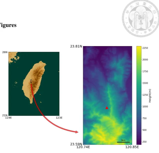
Figure 1. Xitou is located on the west side of the central mountain range of Taiwan. It is

a valley opens to its north. The red triangular represents the location of observations used in this study.

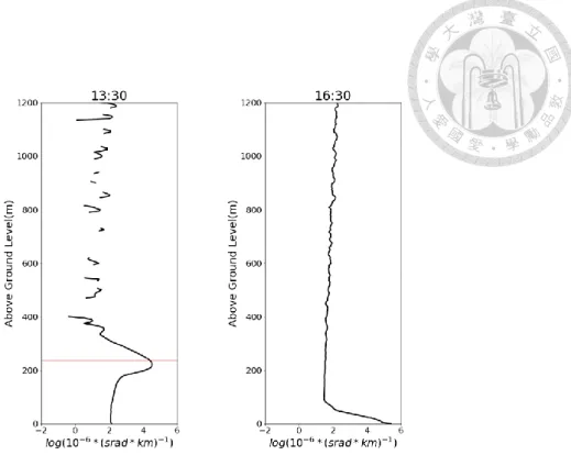
Figure 2. The examples of the backscattering profile observations by Vaisala ceilometer

CL31 when detecting cloud (left) and the fog (right). The red line on the left panel shows the detected cloud base height by ceilometer. When the maximum backscattering intensity is on the ground so that the ceilometer couldn’t detect the cloud base, it will label the

‘DETECTION STATUS' of this data as 4 or more, which is taken as the fog observed on the valley surface in this study.

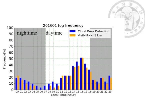
Figure 3. Diurnal variation of fog frequency by ceilometer cloud base detection (blue bar)

and visibility detection (yellow bar) at Xitou for January 2016. The grey shaded areas represent night time at Xitou. The frequency is defined by the ratio of the amount of data that detecting the fog by instruments and the total observation data count in that hour over the whole January (31 days). By visibility sensor, the fog is defined as the horizontal visibility less than 1 km.

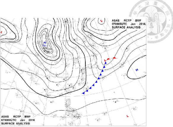
Figure 4. The synoptic surface weather map on Jan 7th, 2016 published by the Central Weather Bureau of Taiwan. The center of Siberian High was at about 49⁰N while its anti- circulation covers almost entire East Asia. The prevailing winds around Taiwan were northeastern winds; it was about 15 knots over the east coast of Taiwan while less than 5

vii

knots on the Xitou valley and western plain of Taiwan. The weather of the Xitou valley and western plain of Taiwan was somewhat stable without the influence of the synoptic weather system, which resulted in a weather regime mainly controlled by the local effects of complex topography.

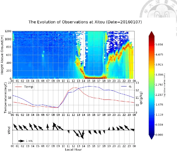
Figure 5. The evolutions of backscatter profile (upper panel), surface temperature (red

line in the middle panel), surface water vapor mixing ratio (blue line in the middle panel), and surface wind (lower panel) on Jan 7th, 2016. The ‘-‘ and ‘x’ markers in the upper panel represent low-level cloud base height and the fog detected by the ceilometer. It shows that from the early morning to the noon, the sky of Xitou is cloudless, so that backscattering profiles show little signals and the temperature rose from around 12 ⁰C (9 am) to 20 ⁰C (12 pm). The low-level clouds formed between 12 and 1 pm and the ceilometer detected the cloud base at around 400m above the ground. The cloud base was lowering gradually to the ground resulted in fog formation at Xitou valley at 2:20 pm.

The fog sustained for about 4 hours then the backscattering profiles indicate the cloud base elevated after 6 pm. In the lower panel, the local circulation is mainly dominated by the mountain-valley system, in which the mountain winds (SSE winds) blow through the entire nighttime and the morning while the valley winds (NNW winds) initiated at 11 am and continued to late afternoon then turned to the mountain wind at 7 pm. The evolution of surface water vapor mixing ratio (middle panel) also shows that after the low-level clouds formation the moisture of valley surface air was still increasing until 3 pm.

Figure 6. The skew-T plot of sounding at Ishigakijima, Japan on Jan. 7th, 2016. The

inversion strength is objectively defined by the temperature inversion at 2700 m. The potential temperature difference between 2700 m to 2900 m is about 10K and the water vapor mixing ratio drop dramatically from 6 g kg^-1 to less than 0.5 g kg^-1. The inversion strength is set to 50 K km^-1 for our experiment.

Figure 7. The initial potential temperature (left) and water vapor mixing ratio (right)

profiles for idealized experiments. The inversion strength in four experiments is set to be 10K (red), 8K (orange), 5K(green), and 3K (blue) from 2700 m to 2900 m. The inversion strength is 50 K km^-1, 40 K km^-1, 25 K km^-1, and 15 K km^-1 respectively. The water vapor mixing ratio profiles in four experiments are set to be the same (black line on the right panel). The 50 K km^-1 inversion strength potential temperature and water vapor mixing ratio profiles are idealized from the sounding at Ishigakijima, Japan on Jan. 7th, 2016 (black dash lines in both panels) so that the simulation of TH10 (CTRL) can represent the local topographic effects of our studying fog event on that day.

Figure 8. The x-z plane flow vector and the cloud water mixing ratio distribution along

the cross-section of the Xitou valley at 12 pm in experiment TH10(CTRL). It shows that the leading edge of valley winds lifted by valley bottom surface then induced convections.

The capping inversion layer on 3200m limited the convections so that the cloud water accumulated around 2000 to 3200 m.

Figure 9. The wind fields (barbs) and water vapor mixing ratio (shaded) on the bottom of the valley (1300 m, upper row) and the top of the valley (2000 m, lower row) at 10 am (left column) and 3 pm (right column) in experiment TH10(CTRL). The gray shaded areas

ix

and contours in the upper panels represent the topography of ridges higher than 1300 m surrounding the Xitou valley. The black (red) boxes in the upper (lower) panels show the Xitou valley area where moisture could be trapped. The upper panels show that the persistent valley winds on the surface of the valley carried moisture into the valley so that the water vapor mixing ratio increased in the lower part of the valley from 10 am (upper left panel) to 3 pm (upper right panel). The lower panels show that on the level of 2000 m, which is higher than the surrounding ridges, the moisture also increased from 10 am (lower left panel) to 3 pm (lower right panel). The wind fields also show that the depth of valley winds are shallow and only exist on the surface of the valley.

Figure10. The evolutions of the liquid water path (red line) and precipitation (green line

in the upper panel), liquid water profile along with cloud base height (middle panel), and surface valley wind strength (lower panel) of the valley in experiment TH10(CTRL). The continuous valley winds initiated right after sunrise and strengthened in the daytime (lower panel). The convections initiated by valley winds resulted in the condensation of the cloud liquid water (middle panel). The dense cloud liquid water accumulated right below strong inversion at the level of 3200 m at the beginning so that the cloud base height (red dashed line) and its hourly mean (black line in the middle panel) is at around 2000 m in the morning. Then with more liquid water condensed in the late afternoon, cloud base height lowered to the ground at around 6 pm. The upper panel shows that the precipitation and liquid water path increased along with the lowering of cloud base height in the late afternoon.

Figure 11. The three-dimensional flow structure over the Xitou complex terrain in

experiment TH10(CTRL). Different colors of streamlines represent separate air parcels sampled in the valley. It shows that the upslope valley winds converged into the valley surface. The air parcels uplifted by valley bottom topography and convections initiated.

The flows then twisted up while upward developing to the level of inversion. The capping inversion prohibited the further development of convections so that the air parcels flowed out the valley horizontally.

Figure 12. The fog duration of four experiments. The experiment TH03 with the inversion

strength set to only 3 K within 200 m (15 K km^-1 respectively) results in the fog duration lasting less than one hour. The fog durations are gradually increasing with the prescribing inversion strength systematically. With stronger inversion strengths as 8K and 10K, The resulting fog durations could be apparent longer than 7 hours.

Figure 13. The evolutions of the liquid water path of experiment TH03, TH05, TH08,

and TH10. The liquid water path in the experiment TH03 is under 4 g m^-2 in the whole simulation daytime period and shows no significant changes. On the other hand, the liquid water path increased approximately 7g m^-2 in the late afternoon in both the experiments TH10 (CTRL) and TH08. The liquid water path in the experiment TH05 also gradually increased in the afternoon and the maximum value of it is in between of the results in experiment TH08 and TH03.

Figure 14. The comparison of wind fields (barbs) and water vapor mixing ratio (shaded) on the bottom of valley (1300m, upper row) and the top of valley (2000m, lower row) at 10 am (left column) and 3 pm (right column) between experiment TH03 (left), TH08

xi

(middle), and TH10 (right) at 3 pm. The gray shaded areas and contours in the upper panels represent the topography of ridges higher than 1300 m surrounding the Xitou valley. The black (red) boxes in the upper (lower) panels show the Xitou valley area where moisture could be trapped. The water vapor mixing ratio of experiment TH03 is the driest case whether on the bottom (upper panels) or top (lower panels) of the valley while the wind fields on the bottom of the valley (upper panels) suggest that the valley winds in the experiment TH03 is comparable with experiment TH08 and TH10 (CTRL).

Figure 15. The potential temperature (left), water vapor mixing ratio (middle), and liquid

water mixing ratio (right) profiles of the boundary layer at 11 am of experiment TH03 (blue), TH05 (green), TH08(orange), and TH10 (red). The potential temperature profile of experiment TH03 shows that the prescribe inversion had been smeared so that convections could develop up to higher than 3000 m and more moisture is carried upward to a more upper atmosphere. On the contrast, the potential temperature profiles of the other experiments show that the inversion strengths are strong enough to limit convections so that the condensed liquid water only exists below the inversion layer and the water vapor suddenly dropped above the inversion level.

Figure 16. A schematic of the upslope fog formation processes at Xitou valley. The

upslope winds and the convections moisten the valley boundary layer so that the low- level clouds form and consequently reduce the insolation. With the capping inversion to confine the moisture in the valley, the accumulation of moisture keeps lowering the cloud base to the ground become the fog.

Table captions

Table 1. The setting of the inversion strength for four idealized experiments. The differences of the potential temperature are set in between 2700 m to 2900 m of the initial profiles.

1

1. Introduction

Montane cloud forests are characterized by forests that are frequently immersed in clouds or fog. This environment allows the canopy to intercept cloud or fog water, which contributes extra hydrological input to the ecosystem (Dawson, 1998; Scholl et al., 2011).

This unique hydrological process makes the distribution of montane cloud forest sensitive not only to precipitation and temperature but also to the frequency of cloud or fog occurrence. Still et al. (1999) showed that under global warming scenario, the rise of cloud base height could lead to an upward shift of montane cloud forest. Moreover, this impact over complex topography could potentially result in not only the shrinking but also fragmentation of the montane cloud forest (Bruijnzeel, 2001). Since Taiwan is an island with complex topography and the forests covering more than 50% of its land area (Lu et al., 2000), the fragmentation and shrinking of montane cloud forests could be severe issues associated with climate change. It is necessary to estimate the area of cloud forests coverage first to measure the actual changes of cloud forests area in Taiwan.

Schulz et al. (2015, 2017) demonstrated that the detection of the fog areas and mapping the cloud forest distribution could be estimated through the satellite data in Taiwan.

However, it is very challenging for satellite observation to discriminate between the fog

and the low-level clouds. Traditionally, the fog is defined by the reduction of horizontal visibility to be less than 1 km. Since the fog is a phenomenon occurring in the boundary layer, the evolution of the low-level clouds might reveal some information associated with the fog formation. Nowak et al. (2008) suggested that the ground-based remote sensing equipment is suitable for detecting the fog event and the low-level cloud base at the same time. Their approach provides a better way to examine the connection between the evolutions of low-level clouds and the fog.

Taiwan is a subtropical island located in East Asia with a maximum elevation near 4000 m above sea level and more than 200 peaks above 3000 m above sea level. The precipitation of the whole island is more than 2000 mm per year (Central Weather Bureau, 2018). Xitou valley, which is located at 1150 m on the west slope of the Central Mountain Range in Taiwan (Fig. 1), is one of the most intensive montane fog studying areas in Taiwan. Liang et al. (2009) reported 320 foggy days with 2415 foggy hours or 28% of the whole year sampling time from April 2005 to March 2006. The following study by Wey et al. (2011) showed that the days of fog occurrence are 292 days in the sampling year

(February 2011 to January 2012). They also found that the fog in Xitou valley tends to form in the afternoon and dissipate after the sunset. The characteristics of the diurnal cycle of the fog are robust in all seasons. After a more detail, statistical analysis of local

3

wind in the same period of the fog observations, Wey et al. (2016) found that the diurnal cycle of the fog formation and dissipation are consistent with the mountain-valley winds system of Xitou valley. They concluded that the mountain-valley wind system is the crucial factor to fog formation at Xitou and they classified the fog of Xitou valley as the upslope fog. The concept of the upslope fog is that the moisture supplying by the upslope valley winds in the daytime leads to the fog formation in the valley. However, the aforementioned observational studies with little information about the moisture transport processes are challenging to evaluate the moistening effects by the upslope winds so that the relationship between the upslope winds and the fog occurrence frequency or fog duration is still not clear. To further investigate the moisture transport processes associated with the orographic induced flow the numerical simulation experiment is needed. Wilson and Barros (2015, 2017) used the Advanced Weather Research and Forecasting (WRF) model simulation to study the warm season orographic rainfall in the southern Appalachians. Their results showed that the low-level moisture convergence controlled by topography is a necessary precursor to valley fog and low-level cloud

formation.

To understand how the orographically induced low-level moisture convergence control to the fog occurrence and its duration, in this study, we inspect the boundary layer

by probing the low-level could base evolution and the fog formation through ceilometer and investigating the vertical distribution and development of the moisture by idealized simulation. This study is the first attempt to understand the local circulation associated with fog at Xitou using a high-resolution cloud-resolving model. The description of the studying area and the observations are presented in section 2. The analysis of observations and case study are in section 3. The model description and the design of the idealized simulations from the case study are presented in section 4. The simulated results are presented in section 5. A summary and discussion are given in section 6.

5

2. Study Area and Observations

Xitou valley is the basin of the Beishi River, which is the branch of the Zhuoshui River. The V-shaped Xitou valley is bounded by surrounding mountains on the west, south, and east sides and opens to the north. The elevations of the surrounding peaks are from 1500 m to 2000 m approximately. The heights of the valley bottom are 600 m on the north part and elevated gradually to 1200 m on the south edge. The width of Xitou valley is about 4 km, and the valley is 10 km long from north to south. The surface observation site is located at the Xitou Nursery of National Taiwan University Experimental Forest (1150 m). The Agricultural Meteorological Station (AMS) is set at the Nursery along with the visibility sensor to detect fog. In this study, we use the surface temperature, humidity, wind, and visibility data from this observation site.

Besides all the in-situ observation instruments mentioned above, a Vaisala Ceilometer CL31 was also set next to the AMS since November 2015. This system implements light detection and ranging technology, in which short, powerful laser pulse is sent out vertically into the atmosphere. The reflection of light caused by aerosol, fog, cloud, or precipitation is measured as the laser pulse traverse the sky, called backscatter.

The resulting backscatter strength profile with height is stored and processed to identify

the cloud base. The ceilometer can discriminate between three layers of cloud at most and label it as ‘DETECTION STATUS’ along with backscatter profile as output. When the lowest cloud base is close to the ground, the data processing unit labels ‘DETECTION STATUS' as 4 or more, which is taken as the fog observed on the valley surface in this study. The example backscattering profiles of cloud and fog detected by ceilometer are shown in Fig. 2.

With the detection of the fog and the cloud base height through ceilometer, we can get more observations related to the vertical evolution of the liquid water in the boundary layer. The fog duration and the cloud base evolution before and after the fog events can also be determined. The frequency of surface observations is hourly which is suitable to capture the diurnal cycle of dynamic and thermodynamic characteristics in the valley. The sampling frequency of the ceilometer is 5 seconds. By smoothing out the higher frequency signals, the evolution of the backscattering profile presented in this study is every 10 minutes so that we can focus on the more sustain changes of the cloud base height associated with the moisture distribution of the valley. The 10-minute frequency of the

ceilometer data is sufficient to examine the rapid evolutions of the cloud base. Meanwhile, a visibility sensor is set on the same location of the ceilometer to validate the fog duration and fog occurrence frequency identified by ceilometer.

7

3. Analysis of Observations and Case Study

With high frequency (10 minutes) fog observation by ceilometer, we first analyze the diurnal cycle of the fog occurrence at Xitou. Fig. 3 shows the diurnal fog frequency of January 2016. The results suggest that the fog occurrence in the afternoon is robust at Xitou, which is consistent with previous observational studies. To validate the fog observation by ceilometer, Fig. 3 also shows the fog occurrence frequency identified by the horizontal visibility sensor. The comparison shows high agreement between two instruments so that we are confident that the ceilometer is reliable to detect the fog. To further examine the fog formation processes and the diurnal cycle of the local mountain- valley wind system, we choose a fog event on Jan. 7th, 2016 as our studying case. The synoptic weather environment on Jan. 7th, 2016 is a typical wintertime weather regime, in which Siberian High stays on the east-Asia continent and its anti-cyclonic circulation results in the prevailing northeast winds around Taiwan (Fig. 4). Under this weather regime, the prevailing northeast winds on the east coast of Taiwan is about 15 knots while the surface wind speed around Xitou valley and the western plain of Taiwan, which locate at the lee side of Central Mountain Range of Taiwan, is less than 5 knots due to the topographic blocking effect. The weak prevailing winds allow us to inspect the mountain-

valley wind system development on the Xitou valley without considering the component of the synoptic winds. Fig. 5 shows the evolutions of backscattering profiles and surface observations of the fog case on Jan. 7th, 2016. With ceilometer observations, the backscattering profiles revealed more details of the diurnal cycle of low-level clouds and fog evolutions. In Fig. 5 the duration of low-level clouds and the fog is consistent with the period of local valley winds. The initiation of valley winds is at 11 am, which is an hour earlier than the low-level cloud formation (12 pm), and the timing of the fog dissipating and the cloud base elevating are coincident with the transition of local winds from valley winds to mountain winds (6 pm). In the morning, the surface temperature raised from around 12 ⁰C (9 am) to 20 ⁰C (12 pm). At noon the low-level clouds formed and screened the insolation so that the temperature started to decrease gradually to 15.16⁰C (6 pm) in the afternoon. The increasing of the water vapor mixing ratio in the morning is consistent with the temperature rise, but in the afternoon the moisture still increased slightly while the temperature dropped. The sustained moistening is related to the moisture transport of the valley winds, which we examine by simulations and the

results are discussed in the following sections. Both of the moistening and the declining of the surface temperature promoted the fog formation near the valley surface in the afternoon. By applying ceilometer, the observations show that the characteristics of the

9

evolution of the local low-level clouds and fog are coincident with the valley winds. The clouds or fog also influence the solar radiative heating on the valley surface, which is an essential factor to the local mountain-valley wind system. The interactions among these processes are worthy of being further examined.

It is also worth noting that the skew-T plot of sounding at Ishigakijima, Japan on Jan.

7th, 2016 (Fig. 6) shows that there is a strong temperature inversion above 2700 m. The inversion characteristics of sounding profiles can be identified in 10 fog events out of the total 13 fog events in January 2016 without the influence by the frontal system. Recently through UAV and ceilometer observations analysis also found that the inversion layer on the top of the boundary layer can block the uprising of the cloud water of the convections at Xitou (Lai, personal communication). These observations and our studying event consistently indicate that the inversion might be an essential synoptic control to local fog phenomenon.

The aforementioned observational analysis shows that there should be processes that connect the local valley winds, cloud base lowering and the fog formation. The clear sky

of Xitou valley in the morning enhanced the heating difference over topography by the solar radiation, and the valley winds initiated consequently. The moisture supply and

vertical turbulence mixing induced by valley winds flowing into the valley should be key factors to explain the associated low-level cloud and the fog formation processes.

11

4. Model Description and Experiments Setup

Although the observations related to the time evolution of the cloud base above Xitou valley are collected by ceilometer, it is still difficult to measure the vertical turbulence and moisture fluxes as well as the moisture transport in the valley associated with the mountain-valley wind system. The orographic effects on low-level moisture convergence associated with the upslope winds are still not evident. Therefore, we design numerical simulations of fog formation processes to evaluate the local circulation. Using three-dimensional operational weather prediction model to simulate small scale valley fog event is still very challenging mainly caused by the use of coarser resolutions in both the horizontal and the vertical grids. Modified grid resolutions also influence significantly the parameterization of the model physics, such as the turbulence and heat and moist fluxes at the surface that in turn affect the fog evolution (Gultepe et al., 2007). Moreover, the simulation of orographic fog may only be possible if the model is capable of accurately treating three-dimensional flow over a complex terrain surface (Terra et al., 2004). To minimize the uncertainty of fog simulation caused by the accuracy of flow structure on complex topography, we design a series of idealized cloud-resolving simulation on complex topography of Taiwan by vector vorticity equation cloud-

resolving model (TaiwanVVM).

The model was first developed by Jung and Arakawa (2008) based on the three- dimensional anelastic vorticity equations. This model predicts the horizontal components of vorticity and diagnoses the vertical velocity using a three-dimensional elliptic equation.

The physics parameterizations include: a radiation parameterization using Rapid Radiative Transfer Model for GCMs (RRTMG; Iacono et al., 2008); a bulk three phase cloud microphysics parameterization including cloud droplets, ice crystals, rain, snow and graupel (Krueger et al., 1995); a surface flux parameterization (Deardorff, 1972) and a first-order turbulence closure that uses eddy viscosity and diffusivity coefficients depending on deformation and stability (Shutts and Gray, 1994). On the representation of topography, Wu and Arakawa (2011) apply a block mountain approach in height coordinate in TaiwanVVM, which is capable of reducing numerical errors over steep mountains. It is also shown that TaiwanVVM with this representation of topography approach can simulate mountain waves, orographic precipitation, and downslope wind reasonably and have no computational problems (Wu and Arakawa, 2011, Chien and Wu,

2016). This model has also been used to investigate the influences of boundary layer processes and the environmental conditions on the maintenance of advection fog (Lin., 2015). To examine cloud processes specifically over Taiwan, Wu et al. (2019) design a

13

framework called TaiwanVVM in which the Noah LSM version 3.4.1 (Chen et al. 1996) with high-resolution (500 m) land use data is implemented carefully in the model to match the feature of Taiwan topography. We follow the same settings except for different initial conditions. The setup of simulation resolution is 500 m horizontally, while vertical resolution is 100m from the surface up to 4000 m, above 4000 m is stretching grid up to 17 km, and the total vertical layers are 60 layers. The domain size is 512 by 512 km² and is doubly periodic in the horizontal. This use of high-resolution grid size covering entire Taiwan area and surrounding seas is to avoid domain boundary being cut at the edge complex topography inside Taiwan which potentially can cause problems from the inflow outside of the domain. The integration time step is 10 seconds, and all simulations are integrated for 24 hours starting at midnight. The hours before dawn can be regarded as spinning up time.

To simulate the topographic effects under the synoptic condition of the fog event, we idealized the sounding of this date (Fig. 6) as the initial condition of our idealized experiment. A potential temperature profile with strong inversion (50 K km^-1) at 2700 m

is given as the initial condition of TaiwanVVM to simulate the development of the boundary layer of Xitou valley, which is named TH10 in our study. (Table 1 and Fig. 7).

The initial wind profile is set to calm wind condition to represent the observed weak

synoptic flow at Xitou. A series of experiments given different inversion strength was carried out to discuss its impacts on local fog duration at Xitou. Fig. 7 also shows the initial potential temperature and water vapor mixing ratio profiles of the experiments. The moisture profile is fixed while the strengths of inversion were varied as listed in Table 1.

In these idealized simulations, synoptic scale forcing such as the temperature inversion strength is represented by initial conditions, the diurnal evolution of local boundary layer structure over complex topography is resolved and examined.

15

5. Simulation Results

We first examine the result of experiment TH10, which represents the simplified synoptic inversion of our studying upslope fog event. The results demonstrate the moistening processes in the valley after the initiation of valley winds and the vertical turbulences are explicitly simulated. Under the topographic uplifting effect, the convection in the TaiwanVVM model develops. The convection could only develop up to 3000 m because of the limitation by the capping inversion, result in the accumulation of liquid cloud water around 2000 to 3000 m (Fig. 8). The convections moisten the upper part of the valley boundary layer, which is the crucial process of the upslope fog development previous studies did not identify. Fig. 9 shows the evolution of moisture on the lower and upper levels of Xitou valley. The resulting moistening of the valley by both the valley winds and moist convections could be found. The valley winds converge while flowing into the V-shaped valley. The supply of water vapor by the valley winds convergence keeps moistening the bottom of the valley. The water vapor mixing ratio in the valley at 1300 m (black box in Fig.9) increase from 8.12 g kg^-1 (10 am) to 8.75 g kg^-

1 (3 pm). Although the valley winds induced by the heating difference on topography only

exist on the bottom level, the water vapor mixing ratio of the upper level in the valley still

increases gradually (from 6.05 g kg^-1 at 10 am to 7.07 g kg^-1 at 3 pm). It indicates that the moistening of the upper valley level should come from lower level moisture by vertical turbulence mixing and convections. By consistent valley winds and convections development, the moisture transport upward into the upper level of the boundary layer in the valley. The increased condensation of liquid water leads to the thicker low-level clouds and hence the lowering of the cloud base in the afternoon. Eventually, the cloud base touches the ground and the valley fog forms (Fig. 10).

In the experiment TH10 (CTRL), we simulate the orographic effects on low-level moisture convergence and consequently cloud base lowering and the fog formation. The initiation of valley winds in the morning and the cloud base lowering before the fog formation in the afternoon are both consistent with the observations of our studying fog event. Actually, in this experiment, we found that the observed valley winds are only part of the local circulation in the Xitou valley, which also includes the moist convections triggered by the uplifting effect of topography. By prescribing an initial profile with strong inversion as 50 K km^-1, these convections could not penetrate the inversion and make the

moisture confined in the valley to promote the fog formation. Fig.11 demonstrates the schematic of the three-dimensional flow structure of local circulation in the Xitou valley.

The upslope valley winds converge in the valley, twisted up, and initiate convections. The

17

capping inversion confines the convections, and airflows become horizontal after convections developed to the level of inversion. The upslope valley winds observed on the valley surface only reveals part of the whole local circulation. The three-dimensional structure of local circulation over complex topography could be better identified by the high-resolution cloud-resolving simulation.

Since the inversion capping limit convections development and trap the moisture in the valley, it could be a crucial factor to control the duration of the fog. The simulations with varied inversion strength show that the experiment with weaker inversion strength results in a shorter fog duration. For example, the fog is barely formed on the valley surface, and the fog is lasting only 0.67 hours in the experiment which inversion strength is set as weak as 15 K km^-1 (TH03 in Fig. 12). The comparison of the liquid water path evolution of experiments (Fig. 13) suggests that liquid water and moisture could not be held in the valley in experiment TH03. The incapability of trapping moisture in the valley in weak inversion simulation could also be found on the water vapor mixing ratio distribution. Fig.

14 shows the comparison of wind fields and water vapor on the valley bottom level (1300

m) and upper level (2000 m) at 3 pm. The moisture and circulation characteristics of experiment TH08 are similar to the results in experiment TH10. The valley winds and

more humid environment are at the bottom of the valley while the moistening of the upper level could also be found in both experiments.

On the other hand, the results of the weakest inversion strength experiment (TH03) show that the moisture in the upper level of the valley is drier than the other experiments.

At 3 pm, the water vapor mixing ratio at 2000 m (red box in Fig. 14) of TH08 and TH10 experiments are comparable 7.00 and 7.07 g kg^-1 respectively, while it is only 6.33 g kg^-

1 in TH03 experiment. It is worth noting that the strength of the capping inversion can

influence the moisture within the boundary layer. By examining the conditions of the boundary layer in the valley (Fig. 15), we found that with stronger capping inversion (more than 25K km^-1 respectively), both the liquid water and water vapor are kept under the inversion layer. In experiment TH03, the prescribed inversion is too weak so that it could be overcome and eliminated by convections. Once the inversion no longer exists, the convections develop to a higher level and transport moisture upward to the free atmosphere. Without the inversion to confine moisture in the valley, the fog is barely formed, and the duration is shorter in the experiment TH03. The sensitivity experiments

suggest that the temperature inversion strength in the Xitou valley is the crucial factor in the duration of the fog.

19

6. Summary and Discussion

Montane cloud forests are characterized by forests which are frequently immersed in clouds or fog. Previous studies suggest that over complex topography the impact of global warming on montane cloud forests could be more serious. It is necessary to understand the orographic effects on fog formation processes to further discuss the impact of climate change. In this study, we validate that the ceilometer is not only reliable to detect fog occurrence but also provides more information about low-level cloud base evolutions. In a fog event on Jan. 7th, 2016, the low-level cloud base lowering is observed before the fog formation, which is also associated with the valley winds at Xitou valley of Taiwan. To understand the orographic effects on moisture convergence and the processes of fog formation, we performed a series of idealized numerical experiments by TaiwanVVM. The simulations demonstrate that the valley winds induced by the heating difference on topography converge the low-level moisture and initiate the convection in the valley. The convection limited by capping inversion keeps the moisture in the valley.

Meanwhile, the formation of the low-level clouds by convections also reduce the insolation heating on the valley surface. The moistening in the valley results in the low- level cloud base lowering, which and the declining of surface temperature both promote

the fog formation. By prescribing four different synoptic inversion strength in the simulations, we also found that the duration of the fog is controlled by the capping inversion strength. The results show that under weak inversion strength the moisture convergence by orographic effects could be transported upward into the free atmosphere so that the fog duration in the valley is reduced. We conclude that orographic effects on low-level moisture convergence are the essential processes to supply moisture in the Xitou valley, and the capping inversion promotes the fog formation by limiting the development of convections and confine moisture in the valley (Fig. 16).

The TaiwanVVM framework applied in this study allows us to use initial conditions as representatives of synoptic forcing to simulate the boundary layer eddy development and evaluate its interactions with complex orography. To assess the potential impact of global warming to local orographic fog at Xitou, we need to apply the current climate and future projection scenarios as the synoptic forcing to our framework. With enough semi- realistic experiments, the local responses of the current climate could be evaluated by the statistical characteristics of simulation results. The potential impact of the future climate

can therefore be examined through the changes of the local upslope fog. The following work will focus on applying the semi-realistic simulation strategy to understand the interaction between the orographic effects and future climate change scenarios.

21

Reference

1. Bruijnzeel, L. A., 2001: Hydrology of tropical montane cloud forests: A Reassessment. Land Use and Water Resources Research, 1, 1.1.

2. Central Weather Bureau, 2018: Climate Monitoring 2017 Annual Report, Central Weather Bureau, Taipei, Taiwan, 43 pp., Chinese, available at:

https://www.cwb.gov.tw/V7/service/notice/download/publish_20181011155441.pd f.

3. Chen, F., and Coauthors, 1996: Modeling of land surface evaporation by four schemes and comparison with FIFE observations. Journal of Geophysical Research:

Atmospheres, 101, 7251–7268, doi:10.1029/95JD02165.

4. Chien, M.-H., and C.-M. Wu, 2016: Representation of topography by partial steps using the immersed boundary method in a vector vorticity equation model (VVM):

VVM PARTIAL STEP. Journal of Advances in Modeling Earth Systems, 8, 212–

223, doi:10.1002/2015MS000514.

5. Clyne, J., and M. Rast, 2005: A prototype discovery environment for analyzing and visualizing terascale turbulent fluid flow simulations. R.F. Erbacher, J.C. Roberts, M.T. Grohn, and K. Borner, Eds., Electronic Imaging 2005, San Jose, CA, 284 http://proceedings.spiedigitallibrary.org/proceeding.aspx?doi=10.1117/12.586032.

6. Clyne, J., P. Mininni, A. Norton, and M. Rast, 2007: Interactive desktop analysis of high resolution simulations: application to turbulent plume dynamics and current sheet formation. New J. Phys., 9, 301–301, doi:10.1088/1367-2630/9/8/301.

7. Dawson, T. E., 1998: Fog in the California redwood forest: ecosystem inputs and use by plants. Oecologia, 117, 476–485, doi:10.1007/s004420050683.

8. De Wekker, S. F. J., and M. Kossmann, 2015: Convective Boundary Layer Heights Over Mountainous Terrain—A Review of Concepts. Frontiers in Earth Science, 3, doi:10.3389/feart.2015.00077.

9. Deardorff, J. W., 1972: Parameterization of the Planetary Boundary layer for Use in General Circulation Models. Mon. Wea. Rev., 100, 93–106, doi:10.1175/1520- 0493(1972)100<0093:POTPBL>2.3.CO;2.

10. Gultepe, I., and Coauthors, 2007: Fog Research: A Review of Past Achievements and Future Perspectives. Pure appl. geophys., 164, 1121–1159, doi:10.1007/s00024- 007-0211-x.

11. Iacono, M. J., J. S. Delamere, E. J. Mlawer, M. W. Shephard, S. A. Clough, and W.

23

D. Collins, 2008: Radiative forcing by long-lived greenhouse gases: Calculations with the AER radiative transfer models. Journal of Geophysical Research, 113, doi:10.1029/2008JD009944.

12. Jung, J.-H., and A. Arakawa, 2008: A Three-Dimensional Anelastic Model Based on the Vorticity Equation. Mon. Wea. Rev., 136, 276–294, doi:10.1175/2007MWR2095.1.

13. Krueger, S. K., Q. Fu, K. N. Liou, and H.-N. S. Chin, 1995: Improvements of an Ice- Phase Microphysics Parameterization for Use in Numerical Simulations of Tropical Convection. Journal of Applied Meteorology, 34, 281–287, doi:10.1175/1520-0450- 34.1.281.

14. Liang, Y.-L., T.-C. Lin, J.-L. Hwong, N.-H. Lin, and C.-P. Wang, 2009: Fog and Precipitation Chemistry at a Mid-land Forest in Central Taiwan. Journal of Environment Quality, 38, 627, doi:10.2134/jeq2007.0410.

15. Lin C.-A., 2015: The influence of near-surface boundary layer conditions on the advection fog. M.S. thesis, Department of Atmospheric Sciences, National Taiwan University, Taiwan, 62 pp.

16. Lu, S.-Y., K.-J., Tang, H.-Y., Ku, and H.-H., Huang, 2000: Climatic Conditions of Forested Lands of Taiwan Forestry Research Institute. Taiwan Journal of Forest Science, 15(3), 429–440.

17. Nowak, D., D. Ruffieux, J. L. Agnew, and L. Vuilleumier, 2008: Detection of Fog and Low Cloud Boundaries with Ground-Based Remote Sensing Systems. Journal of Atmospheric and Oceanic Technology, 25, 1357–1368, doi:10.1175/2007JTECHA950.1.

18. Scholl, M., W. Eugster, and R. Burkard, 2011: Understanding the role of fog in forest hydrology: stable isotopes as tools for determining input and partitioning of cloud water in montane forests. Hydrological Processes, 25, 353–366, doi:10.1002/hyp.7762.

19. Schulz, H. M., B. Thies, S.-C. Chang, and J. Bendix, 2015: Detection of ground fog in mountainous areas from MODIS day-time data using a statistical approach.

Atmospheric Measurement Techniques Discussions, 8, 12155–12201, doi:10.5194/amtd-8-12155-2015.

20. Schulz, H. M., C.-F. Li, B. Thies, S.-C. Chang, and J. Bendix, 2017: Mapping the montane cloud forest of Taiwan using 12 year MODIS-derived ground fog frequency data. PLOS ONE, 12, e0172663, doi:10.1371/journal.pone.0172663.

21. Shutts, G. J., and M. E. B. Gray, 1994: A numerical modelling study of the geostrophic adjustment process following deep convection. Quarterly Journal of the

Royal Meteorological Society, 120, 1145–1178, doi:10.1002/qj.49712051903.

22. Still, C. J., P. N. Foster, and S. H. Schneider, 1999: Simulating the effects of climate change on tropical montane cloud forests. Nature, 398, 608.

23. Terra, R., 2004: PBL Stratiform Cloud Inhomogeneities Thermally Induced by the Orography: A Parameterization for Climate Models. J. Atmos. Sci., 61, 644–663, doi:10.1175/1520-0469(2004)061<0644:PSCITI>2.0.CO;2.

24. Vaisala Oyj Corporation, 2006: Vaisala Ceilometer CL31 Users Guide, Vaisala Oyj Corporation, Vantaa, Finland.

25. Wey, T.-H., Y.-J., Lai, C.-S., Chang, C.-W., Shen, C.-Y., Hong, Y.-N. Wand, and M.- C., Chen, 2011: Preliminary Studies on Fog Characteristics at Xitou Region of Central Taiwan, Journal of the Experimental Forest of National Taiwan University, 25:149–160, Chinese.

26. Wey, T.-H., Y.-J., Lai, M.-C., Chen, and P.-H., Lin, 2016: The Studies on the Relationship Between Mountain Valley Breeze and Upslope Fog at Xitou Region in Central Taiwan, in: Proceeding of the 7th International Conference on Fog, Fog Collection and Dew, Wroclaw, Poland, 24-29 July 2016.

27. Whiteman, C. D., 2000: Mountain Meteorology: Fundamentals and Applications.

Oxford University Press, 376 pp.

28. Wilson, A. M., and A. P. Barros, 2015: Landform controls on low level moisture convergence and the diurnal cycle of warm season orographic rainfall in the Southern Appalachians. Journal of Hydrology, 531, 475–493, doi:10.1016/j.jhydrol.2015.10.068.

29. Wilson, A. M., and A. P. Barros, 2017: Orographic Land–Atmosphere Interactions and the Diurnal Cycle of Low-Level Clouds and Fog. Journal of Hydrometeorology, 18, 1513–1533, doi:10.1175/JHM-D-16-0186.1.

30. Wu, C.-M., and A. Arakawa, 2011: Inclusion of Surface Topography into the Vector Vorticity Equation Model (VVM): Inclusion of Surface Topography into the VVM, Journal of Advances in Modeling Earth Systems, 3(2), doi:10.1029/2011MS000061.

31. Wu, C.-M., H.-C. Lin, F.-Y. Cheng, and M.-H. Chien, 2019: Implementation of the land surface processes into a vector vorticity equation model (VVM) to study its impact on afternoon thunderstorms over complex topography in Taiwan. Asia- Pacific J. Atmos. Sci., accepted.

25

Tables

Table 1. The setting of the inversion strength for four idealized experiments. The differences of the potential temperature are set in between 2700 m to 2900 m of the initial profiles.

EXP Ɵ

TH03 3K

TH05 5K

TH08 8K

TH10(CTRL) 10K

Figures

Figure 1. Xitou is located on the west side of the central mountain range of Taiwan. It is a valley opens to its north. The red triangular represents the location of observations used in this study.

27

Figure 2. The examples of the backscattering profile observations by Vaisala ceilometer

CL31 when detecting cloud (left) and the fog (right). The red line on the left panel shows the detected cloud base height by ceilometer. When the maximum backscattering intensity is on the ground so that the ceilometer couldn’t detect the cloud base, it will label the

‘DETECTION STATUS' of this data as 4 or more, which is taken as the fog observed on the valley surface in this study.

Figure 3. Diurnal variation of fog frequency by ceilometer cloud base detection (blue bar)

and visibility detection (yellow bar) at Xitou for January 2016. The grey shaded areas represent night time at Xitou. The frequency is defined by the ratio of the amount of data that detecting the fog by instruments and the total observation data count in that hour over the whole January (31 days). By visibility sensor, the fog is defined as the horizontal visibility less than 1 km.

nighttime daytime

29

Figure 4. The synoptic surface weather map on Jan 7th, 2016 published by the Central

Weather Bureau of Taiwan. The center of Siberian High was at about 49⁰N while its anti- circulation covers almost entire East Asia. The prevailing winds around Taiwan were northeastern winds; it was about 15 knots over the east coast of Taiwan while less than 5 knots on the Xitou valley and western plain of Taiwan. The weather of the Xitou valley and western plain of Taiwan was somewhat stable without the influence of the synoptic weather system, which resulted in a weather regime mainly controlled by the local effects of complex topography.

Figure 5. The evolutions of backscatter profile (upper panel), surface temperature (red

line in the middle panel), surface water vapor mixing ratio (blue line in the middle panel), and surface wind (lower panel) on Jan 7th, 2016. The ‘-‘ and ‘x’ markers in the upper panel represent low-level cloud base height and the fog detected by the ceilometer. It shows that from the early morning to the noon, the sky of Xitou is cloudless, so that backscattering profiles show little signals and the temperature rose from around 12 ⁰C (9 am) to 20 ⁰C (12 pm). The low-level clouds formed between 12 and 1 pm and the ceilometer detected the cloud base at around 400m above the ground. The cloud base was lowering gradually to the ground resulted in fog formation at Xitou valley at 2:20 pm.

The fog sustained for about 4 hours then the backscattering profiles indicate the cloud base elevated after 6 pm. In the lower panel, the local circulation is mainly dominated by the mountain-valley system, in which the mountain winds (SSE winds) blow through the

31

entire nighttime and the morning while the valley winds (NNW winds) initiated at 11 am and continued to late afternoon then turned to the mountain wind at 7 pm. The evolution of surface water vapor mixing ratio (middle panel) also shows that after the low-level clouds formation the moisture of valley surface air was still increasing until 3 pm.

Figure 6. The skew-T plot of sounding at Ishigakijima, Japan on Jan. 7th, 2016. The

inversion strength is objectively defined by the temperature inversion at 2700 m. The potential temperature difference between 2700 m to 2900 m is about 10K and the water vapor mixing ratio drop dramatically from 6 g kg^-1 to less than 0.5 g kg^-1. The inversion strength is set to 50 K km^-1 for our experiment.

33

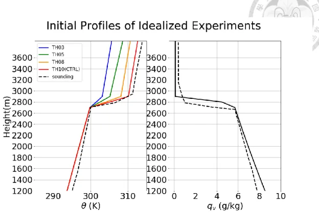
Figure 7. The initial potential temperature (left) and water vapor mixing ratio (right)

profiles for idealized experiments. The inversion strength in four experiments is set to be 10K (red), 8K (orange), 5K(green), and 3K (blue) from 2700 m to 2900 m. The inversion strength is 50 K km^-1, 40 K km^-1, 25 K km^-1, and 15 K km^-1 respectively. The water vapor mixing ratio profiles in four experiments are set to be the same (black line on the right panel). The 50 K km^-1 inversion strength potential temperature and water vapor mixing ratio profiles are idealized from the sounding at Ishigakijima, Japan on Jan. 7th, 2016 (black dash lines in both panels) so that the simulation of TH10 (CTRL) can represent the local topographic effects of our studying fog event on that day.

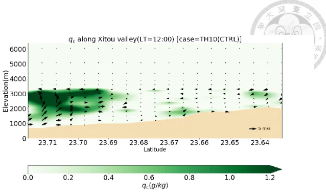
Figure 8. The x-z plane flow vector and the cloud water mixing ratio distribution along

the cross-section of the Xitou valley at 12 pm in experiment TH10(CTRL). It shows that the leading edge of valley winds lifted by valley bottom surface then induced convections.

The capping inversion layer on 3200m limited the convections so that the cloud water accumulated around 2000 to 3200 m.

35

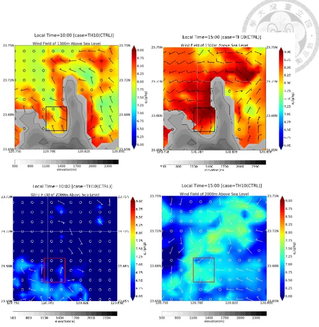
Figure 9. The wind fields (barbs) and water vapor mixing ratio (shaded) on the bottom

of the valley (1300 m, upper row) and the top of the valley (2000 m, lower row) at 10 am (left column) and 3 pm (right column) in experiment TH10(CTRL). The gray shaded areas and contours in the upper panels represent the topography of ridges higher than 1300 m surrounding the Xitou valley. The black (red) boxes in the upper (lower) panels show the Xitou valley area where moisture could be trapped. The upper panels show that the persistent valley winds on the surface of the valley carried moisture into the valley so that the water vapor mixing ratio increased in the lower part of the valley from 10 am (upper left panel) to 3 pm (upper right panel). The lower panels show that on the level of 2000

m, which is higher than the surrounding ridges, the moisture also increased from 10 am (lower left panel) to 3 pm (lower right panel). The wind fields also show that the depth of valley winds are shallow and only exist on the surface of the valley.

37

Figure 10. The evolutions of the liquid water path (red line) and precipitation (green line

in the upper panel), liquid water profile along with cloud base height (middle panel), and surface valley wind strength (lower panel) of the valley in experiment TH10(CTRL). The continuous valley winds initiated right after sunrise and strengthened in the daytime (lower panel). The convections initiated by valley winds resulted in the condensation of the cloud liquid water (middle panel). The dense cloud liquid water accumulated right below strong inversion at the level of 3200 m at the beginning so that the cloud base height (red dashed line) and its hourly mean (black line in the middle panel) is at around 2000 m in the morning. Then with more liquid water condensed in the late afternoon, cloud base height lowered to the ground at around 6 pm. The upper panel shows that the precipitation and liquid water path increased along with the lowering of cloud base height in the late afternoon.

Figure 11. The three-dimensional flow structure over the Xitou complex terrain in

experiment TH10(CTRL). Different colors of streamlines represent separate air parcels sampled in the valley. It shows that the upslope valley winds converged into the valley surface. The air parcels uplifted by valley bottom topography and convections initiated.

The flows then twisted up while upward developing to the level of inversion. The capping inversion prohibited the further development of convections so that the air parcels flowed out the valley horizontally.

39

Figure 12. The fog duration of four experiments. The experiment TH03 with the inversion

strength set to only 3 K within 200 m (15 K km^-1 respectively) results in the fog duration lasting less than one hour. The fog durations are gradually increasing with the prescribing inversion strength systematically. With stronger inversion strengths as 8K and 10K, The resulting fog durations could be apparent longer than 7 hours.

Figure 13. The evolutions of liquid water path of experiment TH03, TH05, TH08, and

TH10. The liquid water path in the experiment TH03 is under 4 g m^-2 in the whole simulation daytime period and shows no significant changes. On the other hand, the liquid water path increased approximately 7g m^-2 in the late afternoon in both the experiments TH10 (CTRL) and TH08. The liquid water path in the experiment TH05 also gradually increased in the afternoon and the maximum value of it is in between of the results in experiment TH08 and TH03.

41

Figure 14. The comparison of wind fields (barbs) and water vapor mixing ratio (shaded)

on the bottom of valley (1300m, upper row) and the top of valley (2000m, lower row) at 10 am (left column) and 3 pm (right column) between experiment TH03 (left), TH08 (middle), and TH10 (right) at 3 pm. The gray shaded areas and contours in the upper panels represent the topography of ridges higher than 1300 m surrounding the Xitou valley. The black (red) boxes in the upper (lower) panels show the Xitou valley area where moisture could be trapped. The water vapor mixing ratio of experiment TH03 is the driest case whether on the bottom (upper panels) or top (lower panels) of the valley while the wind fields on the bottom of the valley (upper panels) suggest that the valley winds in the experiment TH03 is comparable with experiment TH08 and TH10 (CTRL).

Figure 15. The potential temperature (left), water vapor mixing ratio (middle), and liquid

water mixing ratio (right) profiles of the boundary layer at 11 am of experiment TH03 (blue), TH05 (green), TH08(orange), and TH10 (red). The potential temperature profile of experiment TH03 shows that the prescribe inversion had been smeared so that convections could develop up to higher than 3000 m and more moisture is carried upward to a more upper atmosphere. On the contrast, the potential temperature profiles of the other experiments show that the inversion strengths are strong enough to limit convections so that the condensed liquid water only exists below the inversion layer and the water vapor suddenly dropped above the inversion level.

43

Figure 16. A schematic of the upslope fog formation processes at Xitou valley. The

upslope winds and the convections moisten the valley boundary layer so that the low- level clouds form and consequently reduce the insolation. With the capping inversion to confine the moisture in the valley, the accumulation of moisture keeps lowering the cloud base to the ground become the fog.