隨意網路行動模型之機率分析

(1)

行政院國家科學委員會專題研究計畫成果報告

隨意網路行動模型之機率分析研究成果報告(精簡版)

計畫類別：個別型

計畫編號： NSC 96-2221-E-011-037-

執行期間： 96 年 08 月 01 日至 97 年 10 月 31 日執行單位：國立臺灣科技大學電子工程系

計畫主持人：陳維美

計畫參與人員：碩士班研究生-兼任助理人員：吳培源碩士班研究生-兼任助理人員：李圭章博士班研究生-兼任助理人員：黃慕凱

報告附件：出席國際會議研究心得報告及發表論文

公開資訊：本計畫涉及專利或其他智慧財產權，2 年後可公開查詢

中華民國 98 年 01 月 31 日

(2)

行政院國家科學委員會補助專題研究計畫成果報告 隨意網路行動模型之機率分析

計畫編號：96-2221-E-011-037-

執行期限：96 年 08 月 01 日至 97 年 10 月 31 日 主持人：陳維美台灣科技大學電子工程系

計畫參與人員：吳培源黃慕凱李圭章 台灣科技大學電子工程系

摘要

在行動隨意網路(Mobile Ad Hoc Network, MANET) 的環境中，資料的傳遞必需藉由多跳式(multi-hop)的機制來運作，不過在眾多 MANET 網路環境中的路由協定中，皆是以最少跳躍(hop)數為選擇路由路徑的選擇依據，但是這樣的做法卻可能遭遇路由路徑容易斷裂的問題，導致行動節點必需重新找尋路由路徑，不僅浪費無線網路頻寬，也降低了網路產能(throughput)。為加強路由路徑的可靠度，我們提出了分環式(ring-based)路由路徑選擇機制，主要是依據相鄰兩行動節點間連線的存活機率選擇路由路徑，並將此機制實際合併於需求式路由路協定 DSR(Dynamic Source Routing) 上，在 NS2 (Network Simulator ver.2) 網路模擬器進行模擬實驗。由模擬實驗結果顯示，加上分環式路由路徑選擇機制，路由可靠性可有效的提升，並增加網路產能。

一、MANET 網路環境簡介

對於 MANET 網路環境而言，通常具有幾項特性：

 行動節點需擔任路由器的角色：在一個大規模的MANET網路環境中，接收端的行動節點通常不在發送端的傳輸範圍之內，因此在發送端與接收端這兩個行動節點之間，會有一到多個行動節點來擔任轉送的工作，即路由器的角色，所以在MANET裡的每一個行動節點，都要具備所謂的路由(routing)功能。

 行動節點的移動模式無法預測：在MANET中的所有行動節點皆能在任意時間點往任意方向進行移動，因此在MANET網路中，網路拓

樸(topology)會因為行動節點的任意移動而隨時改變的，也因如此，MANET的網路拓樸也變成不可預測的。

 有限的能源(power)：在MANET網路中的行動節點，必需仰賴可攜式的能源裝置提供電源才能正常運作，運作的時間長短，就受限於供電裝置的續航力，不如一般有線網路中的PC，

直接由市電供應能源，無需擔心續航力不足的問題。

 網路頻寬的限制：在MANET網路之中，所以的行動節點間的資料傳輸皆是採用無線傳輸的方式來完成，而在無線網路所使用的頻寬於現今的IEEE 802.11無線技術下，較風行的是 IEEE 802.11b與IEEE 802.11g兩種，其頻寬分別為11Mbps與54Mbps兩種頻寬，但是相較於有線網路的100Mbps或是1Gbps的頻寬之下，

無線網路的頻寬還是較為有限，除此之外，無線網路的環境中，還存在有頻道、頻率等問題，延伸出碰撞(collision)、衰減(fading)及干擾(interference)等等會影響資料傳送的潛在性問題。

除了以上的特點外，MANET網路中，路由協定一般分成兩大類，一為主動式路由協定(proactive routing protocol)，此類的路由協定下，主要的特性是必需週期性地更新每一個行動節點的路由表 (routing table)，所以又稱為表格驅動式路由協定 (table driven routing protocol)，此種作法雖然可以得到較新的路由資訊，但卻相對地浪費網路頻寬；另一種為被動式路由協定(reactive routing protocol)，此類的路由協定相較之下不必週期性地更新路由資

(3)

訊，只有在行動節點有需要，卻沒有路由資訊的情況下才會發動路由路徑的找尋動作，所以又稱為需求式路由協定(on-demand routing protocol)，與主動式路由協定相較之下，比較不會浪費網路頻寬，不過卻有著路由資訊太舊的問題。

二、路由可靠度

在MANET的路由協定中，大部分都是以最短路徑為選擇路由路徑的主要依據，以節省並提高無線網路頻寬的利用。然而，這種路由路徑卻承受著較高的路徑斷裂機率，因此我們將著重於MANET 網路環境中路由路由可靠度(或路徑存活時間)的研究。

如圖1所示，圖中的圓圈範圍代表著行動節點的無線傳輸範圍，假設我們需要從S行動節點到D行動節點間建立一條路由路徑，在MANET網路環境中，我們有兩條路由路徑可以選擇，路徑1從跳躍數目(hop count)觀點來看，是屬於最短路徑，不過卻缺乏可靠度，因為行動節點A非常容易就會漫遊出S 行動節點和D行動節點的無線傳輸範圍，而造成路由路徑斷裂；路徑2可能就會有比較高的可靠度，因為其中間的行動節點B與C在路徑斷裂前，具有較大的漫遊區域可供移動。

圖1 MANET網路環境中路由路徑的可靠度

路由可靠度定義可以在許多相關研究中得到不同的解釋。在ABR[6]路由協定中，每一個行動節點不需擁有路由資訊，而路徑的選擇是建立在所謂的關聯穩定度(association stability)狀態，而此關聯穩定狀態常常會暗示行動節點是否正處於一個穩定的狀態下，因此路徑不需要時常被要求重新更新。在 SSA(Signal Stability-based Adaptive) [2]協定中，在選擇路由路徑時，考慮訊號的穩定度。方向預測的方

法在[5]中被提出，其中也基於兩相鄰行動節點的現在位置、漫遊方向及漫遊速度來定義了路由路徑存活時間，亦被應用在多點傳送(multicast)的環境中 [3]。其它對於路由路徑選擇相關研究有[7][8]等等。

事實上就可靠度而言，選擇路由路徑時所可能參考到的因子有很多，例如路由路徑的長度、路由品質、

訊號強度、路徑頻寬及路徑存活時間等等。

三、分環式路由機制設計

分環式概念是以行動節點為圓心，將無線傳輸範圍以同心圓方式分成若干個環，如圖 2 是以 5 層的環為範例。如有其它行動節點移動到此行動節點的無線傳輸範圍內，此行動節點可依 RSS(Received-Signal-Strength)公式預估與其之間的距離，進而得知其位於那一個環之中。

由於單純只考慮路由路徑長度或是路徑跳躍個數是無法判別路由可靠度的，所以[9]將蜂巢式結構 (cellular structure)化簡後，再進行路徑存活時間的預測，以改進路由可靠度，不過這樣的作法確太過於複雜與不自然。[1]中提出一個環狀蜂巢結構，可應用於預測路徑存活機制，但蜂巢結構與實際應用仍有差距。事實上，在一般簡化的狀況下，任兩行動節點間的距離狀態只會有三種變化，靠近、維持不變以及更遠三種，都是三分之一的機率，若以此來做考量，任兩行動節點間再也不會有方向性的問題，只有相對距離狀態的改變。

圖 2 同心狀分環式結構

(4)

我們做法是依據分環式結構建出連結存在與否的機率模型。如圖 3 所示，任兩個行動節點間距離狀態變化機率之狀態圖，由於行動節點本身有移動的特性，所以相對於自己無線傳輸範圍內的其它行動節點而言，是具有靠近、保持不變及更遠的距離狀態特性，再加上其它行動節點也是具有此特性，所以對於任兩行動節點間的距離狀態共有九種變化，我們是利用此路徑存活機率大小做為路由路徑可靠度選擇的依據。圖 3 是以五環為例，其中的六種狀態為兩行動節點間相距幾個環的狀態，狀態 5和狀態 6 為吸收(absorbing)狀態，如果有某一連結的狀態進入到狀態 5 和狀態 6，我們即把此連結視為斷裂。

圖 3 兩行動節點間距離狀態變化機率之狀態圖

四、分環式路由路徑選擇機制之整合

我們將所提之分環式路由路徑選擇機制整合到MANET網路裡的DSR路由協定中，其主要原因有下列幾點：

 屬於需求式路由協定：需求式路由協定不需定時更新路由表，不會浪費MANET無線網路環境中有限的頻寬，DSR即是典型的需求式路由協定，非常地適合應用在MANET網路環境中。

 可同時維護多條路徑：DSR路由協定具有路由快取(routing cache)機制，可以儲存經由路由探索程序或當資料中繼點時所得知的路由路徑，對於同一個目的地行動節點，可以同時存在一條或多條路由路徑，我們可藉此選擇多條路由路徑中，可靠度最高的路徑。

 具分組轉送機制：不像其它MANET網路中的路由協定是採用逐跳式路由(hop-by-hop)，

DSR是由來源行動節點進行主動尋路的一種無線網路路由技巧，來源行動節點決定了所有封包在傳遞時所需經過的中間行動節點順序，此路由資訊將會被放在封包的頭端(header)

部份，而此封包將會依此順序來傳遞至目的地行動節點。

在機制整合後，路由協定的運作流程圖即如圖 4 所示，來源端行動節點會先行檢查自己的路由快取是否有到目的地行動節點的路由路徑存在，若找不到，則進入路由路徑探索程序；若有找到，則用分環式機制求出所有可到達目的地行動節點之路徑的機率值，並以機率值最大者之路由路徑為封包傳送的路徑。在路由路徑探索程序中，所有在 MANET 網路環境中的行動節點也會以圖 5 之流程圖來進行運作，當任意行動節點收到一個路由請求(Route Request，RREQ)封包時，會先確認自己是否為目的地行動節點，如是，就立即發送路由回應(Route Reply，RREP)封包回來源行動節點；如不是，則檢查自己的路由快取內是否有到目的地行動節點的路由路徑，若沒有則將收到的路由請求封包再往下廣播出去；若是路由快取內有路徑到達目的地行動節點，則依分環式機制求出所有可到達目的地行動節點之路徑的機率值，將機率值最大者之路由路徑放到路由回應封包並發送回來源行動節點。

圖 4 分環式路由機制之流程圖

(5)

圖 5 分環式路由路徑探索程序之流程圖

五、模擬結果

針對我們所提出的無線隨意行動網路之分環式路由機制設計研究中，所提出的分環式路由路徑選擇機制，我們將透過模擬的方式來討論這樣的機制表現結果。在換算實際距離方面，我們使用常被利用來求得距離的有效方法，即是利用無線電訊號隨著距離長度而衰減的特性來求得距離，可依 RSS (Received-Signal-Strength) 得到，只需利用一些已知的訊號衰減公式，即可根據接收到的訊號強度來推估訊號傳遞的距離長度；模擬時包含整體網路環境的產能，進而討論三種封包傳輸間隔時間、五種網路環境密度(density)與四種行動節點移動速度的影響。我們的模擬軟體是採用 NS-2[4]網路模擬器，版本為 2.29 版。

我們所使用的模擬環境範圍是設定於一個 1000平方公尺的平面中，模擬時間設定為200秒，模擬的行動節點個數分別設定為10、20、30、40與50，

行動節點的移動速度分別為5、10、15與20公尺/每秒，每一個行動節點的傳輸半徑為250公尺，傳輸方式則是設定為CBR(Constant Bit Rate)，封包的大小為1024位元組(bytes)，行動節點移動的方向則是採取隨機決定(random way point)，每一進行移動的節點停留時間(pause time)則是設定為10秒，無線網路

的頻寬設定為2Mbps。

每一次模擬會依不同的網路密度而調整行動節點間的通訊連線個數，每一條通訊連線的兩個行動節點是由隨機產生，通訊連線起始時間亦是隨機產生，

並且持續一百秒，以 50 個行動節點的網路模擬為例，會有 25 條隨機配對的通訊傳輸連線，通訊傳輸時間點隨機產生，持續一百秒，並且必需在實驗模擬時間結束前，完成所有通訊傳輸連線；針對通訊連線時，來源行動節點傳送封包的速率，我們也分成每秒 2 個、5 個與 10 個封包的速度，並分別模擬與討論。以上所陳述的數值設定整理於表 1 之中。

模擬環境區域範圍 1000平方公尺

模擬時間 200秒

無線網路頻寬 2Mbps

行動節點個數 10、20、30、40、50

傳送資料的行動節點個數 5、10、15、20、25

傳輸方式 CBR/UDP

行動節點移動模型 Random way point model

行動節點移動速度 5、10、15、20 m/s

停止時間 10秒

封包大小 1024位元組

表1 模擬環境數值設定

我們將所提出之分環式機制，整合到行動節點的無線傳輸範圍，依距離長短將行動節點的無線傳輸範圍等距分成 5、10 與 15 等不同密度的環，並各個別做實驗模擬，並與標準 DSR 路由協定做比較，以了解分環式機制對路由協定的效能之提升。

在行動節點移動速度較慢時，例如移動速度每秒 5 公尺時，如圖 6 所示，分環式機制的路由選擇在效能上比較靠近標準 DSR 協定，主要是因為行動節點移動速度較慢，連結較不易斷裂，相對路由路徑的變化也較少。不過，當行動節點的移動速度再往上調升時，模擬結果也出現較大的轉變，如圖 7、

8 與 9 所示，我們所提之分環式路由機制，確實能增強路由協定的可靠度，進而提升整體網路的產能，如圖 9(a)所示，最高還比標準 DSR 協定高出 19.64%之多的產能，在其它條件下，分環式機制也都有高出 10%以上的表現。圖 6 到圖 9 亦說明加了分環式路由機制的協定，比標準 DSR 協定更適合於

(6)

高移動速度與高資料傳輸流量的網路環境。

20 40 60 80 100 120 140 160

10 20 30 40 50

Number of Nodes

Throughput(Kbits/sec)

5R 10R 15R DSR

(a) 封包傳輸間隔時間0.5s

40 60 80 100 120 140 160 180

10 20 30 40 50

Number of Nodes

5R 10R 15R DSR

(b) 封包傳輸間隔時間0.2s

60 80 100 120 140 160 180

10 20 30 40 50

Number of Nodes

5R 10R 15R DSR

(c) 封包傳輸間隔時間0.1s

圖6 行動節點移動速度每秒5公尺之Throughput比較

20 40 60 80 100 120 140

10 20 30 40 50

Number of Nodes

5Ring 10Ring 15Ring DSR

60 70 80 90 100 110 120 130 140

10 20 30 40 50

Number of Nodes

100 110 120 130 140 150 160 170

10 20 30 40 50

Number of Nodes

20 30 40 50 60 70 80 90 100

10 20 30 40 50

Number of Nodes

Throughput(Kbit/sec)

5R 10R 15R DSR

40 50 60 70 80 90 100 110 120

10 20 30 40 50

Number of Nodes

5R 10R 15R DSR

(7)

0 20 40 60 80 100 120 140 160

10 20 30 40 50

Number of Nodes

5R 10R 15R DSR

20 30 40 50 60 70 80 90

10 20 30 40 50

Number of Node

5R 10R 15R DSR

40 50 60 70 80 90 100 110

10 20 30 40 50

Number of Nodes

5R 10R 15R DSR

60 70 80 90 100 110 120 130 140

10 20 30 40 50

Number of Nodes

5R 10R 15R DSR

六、結論

在 MANET 網路環境中，路由路徑的長度與路由可靠度一直是個兩難的問題，而在眾多 MANET 網路標準路由協定裡，都是以最短路由路徑為優先，在某些網路條件下，例如在行動節點移動速度較快的情況下，這種做法反而沒有效率，而降低網路的產能；我們針對 MANET 網路中路由協定的可靠度問題，提出了一個改良可靠度的路由機制，此機制是藉由將行動節點的資料傳輸範圍分成若干個環狀結構，在路由路徑的選擇時，可依此結構來挑選可靠度較高的連結，如此一來整條路由路徑的可靠度即可提高，模擬實驗結果顯示，加了分環式路由機制的 MANET 路由協定，比原來未加分環式機制的 DSR，最高提升了 19.64%之多的平均網路產能，分環式路徑選擇機制的確可提高路由可靠度。

參考文獻

[1] I. F. Akyildiz, S. M. Ho, and Y.-B. Lin, Movement-Based Location Update and Selective Paging for PCS Networks,

IEEE/ACM Transactions on Networking, vol. 4, no. 4, Aug.

1996.

[2] R. Dube, C. Rais, K. Wang, and S. Tripathi, Signal Stability Based Adaptive Routing (SSA) for Ad-Hoc Mobile Networks, IEEE Personal

Communications, Feb. 1997, pp. 36-45.

[3] S.-J. Lee, W. Su, and M. Gerla, Ad Hoc Wireless Multicast with Mobility prediction, Proceedings

International Conference Computer Communications and Networks, 1999, pp. 4-9.

[4] The network simulator–ns-2,

http://www.isi.edu/nsnam/ns/

[5] W. Su, S.-J. Lee, and M. Gerla, Mobility Prediction in Wireless Networks, Proceedings

IEEE Military Communications Conference, vol.

1, 2000, pp. 491-495.

[6] C.-K. Toh, Associativity-Based Routing for Ad Hoc Mobile Networks,

Springer Wireless Personal Communications, vol. 4, no. 2, Mar.

1997, pp. 103-139.

[7] Z. Wu, H. Song, S. Jiang, and X. Xu, A

(8)

Grid-based Stable Backup Routing Algorithm in MANETs, IEEE Multimedia and Ubiquitous

Engineering, Apr. 2007, pp. 680-685.

[8] J. Wang, and S. Medidi, Density-first Ad-hoc Routing Protocol for MANET,

IEEE Communication Systems Software and Middleware and Workshops, Jan. 2008, pp.

528-535.

[9] Y.-C. Tseng, Y.-F. Li, and Y.-C. Chang, On Route Lifetime in Multihop Mobile Ad Hoc Networks,

IEEE Transactions on Mobile Computing, vol. 2,

no. 4, Dec. 2003.

(9)

這次前往澳洲荷巴特參加 The 2008 International Symposium on Ubiquitous Multimedia Computing (UMC 2008) 國際研討會。會議期間為 2008 年 10 月 13 日至 2008 年 10 月 15 日，並同時包含 UMC 2008 與 CSA 2008 此二研討會，三日會議議題包含下列項目：.

1. Ubiquitous and Pervasive Computing

2. Dependable, Reliable and Autonomic Computing 3. Security and Trust

4. Multimedia

5. Networking and Communications 6. Database and Data Mining

7. Software Engineering

CSA 會議主要探討計算機科學與應用之相關議題，UMC 會議則探討計算機科學於隨處可見的多媒體之應用，諸如無線廣播多媒體、網路搜尋引擎、多媒體影音傳輸及家庭安全系統皆為此會議的探討範圍。

研討會共包含了 18 個 Session。其中對 Session 7、12 及 15 尤感興趣，以下將對各 Session 做進一步地報告。

Session 7 由 Dr. Naveen Chilamkurti 主持，會議中除了探討計算機科學應用於醫療系統，如監測心跳規律性以探知心律等問題外，更有不少論文針對 P2P 網路傳輸提出有效率的資料結構以增加傳輸效率與可靠度。

於 Dr. Nishat Ahmad 主持的 Session 12 中，Mr. Dong-Min Seo 提出了一更有效率的方法動態地更新移動物件之狀況；Mr. Dong-Young Lee 與我們分享了新的 Heterogeneous 安全系統之管理模型；Mr. Foon Chi Francts Chul 則分享了圖像辨識的新技術。

延續 Session12，Dr. Byeong Ho Kang 主持的 Session 15 中進一步地包含了靜態與動態多媒體技術的改善，不僅在圖像辨識領域上，更深入地探討多媒體傳輸效率的改善。此外更探討了 Google 搜尋引擎於中國市場中無法勝過百度搜尋引擎。除了傳統計算機理論，Mr. Surtya Kaewarsa 提出了以類神經網路架構取代傳統計算機架構之電源品質偵測方法。

會議中我們報告所發表的論文「Efficient Perfectly Periodic Scheduling for Data Broadcasting」，與與會者分享了我們在週期性無線廣播傳輸效率改善的技術與成果。

在這三日的研討會中，主要參與了探討計算機科學應用於日常科技之 UMC 2008 研討會，於會議中獲得了許多影像辨識、網路傳輸效能改善以及計算機科學應用於家庭生活與安全等相關新知。參與此會議，感到受益良多，感謝國科會計畫的資助參與這內容豐富的研討會。

(10)

Efficient Perfectly Periodic Scheduling for Data Broadcasting

Wei-Mei Chen and Mu-Kai Huang

Dept. of Electronic Engineering, National Taiwan University of Science and Technology [email protected], [email protected]

Abstract

The perfectly periodic scheduling problem is to schedule a set of jobs such that each job is served occasionally, at fairly regular time intervals. For wireless broadcast systems, when a server periodically broadcasts data to different mobile clients, a perfectly periodic schedule provides no-jitter broadcasting and useful information to reduce power consumption for mobile devices. In this paper, we propose an efficient algorithm to determine a perfectly periodic schedule with low average delay.

Our simulation results show that the new algorithm performs still well when the total requested bandwidth is high and the variance of requested period is large.

1. Introduction

Recently, data broadcasting [10, 12] is an important technology to design mobile computing systems with low power consumption and high bandwidth utilization. When a server broadcasts data to different mobile clients successively and periodically, the mobile clients have to wait for the required data and receive it via broadcast channels [1, 8, 10, 11].

Generally mobile devices are power-limited.

Power consumption is one of the major problems in mobile computing systems. To improve power conservation and broadcast performance for data broadcasting, an effective approach is bandwidth scheduling instead of bandwidth competition.

Schedules can significantly reduce the power

requirement of a mobile client by keeping its radio to

“sleep” for most of idle time. For example, in Bluetooth standard [4], the “Park Mode” and “Sniff Mode” allow mobile clients to sleep in their idle time slots.

In a perfectly periodic schedule, each job is scheduled exactly every some fixed number of time slots [2, 5, 6]. In the perfectly periodic scheduling problem, Bar-Noy [2] first suggested a binary tree-based algorithm to schedule requests with unit length. Dhanakoti et al. [7] proposed a scheme for fault avoidance in 802.11 WLANs by binary-tree-based perfectly periodic scheduling. Later in [5, 6], Brakerski et. al. considered a more general problem for scheduling a set of requests with different lengths and periods. Recently, for the same problem in [5, 6], Patil and Garg [9] proposed an algorithm that schedules n job requests in O(nlogn) time.

For any job requirement, it is not always feasible to determine a perfect schedule which satisfies all requested period. In fact, it is NP-hard even to decide whether a given set of requests admits a perfectly periodic schedule [3]. Thus, one objective of perfect scheduling is to reduce the average delay of jobs.

In this paper we study the perfectly periodic scheduling problem for the client requests with different requested periods and various requested lengths. The rest of this paper is organized as follows.

Preliminaries and related work are introduced in Section 2. In Section 3, we propose an algorithm called GAS for perfectly periodic scheduling.

Performance evaluation is presented in Section 4 and the conclusion is given in Section 5.

2. Preliminaries

This work is supported by National Science Council under the Grant NSC96-2221-E-011-037

2008 International Symposium on Ubiquitous Multimedia Computing

29

(11)

2.1 Problem Statement and Notation

Given a set of n jobs, each job i associated with a requirement (bi, τi), where bi is the length (or execution time) of job i and τi is the requested period of job i. A set of n jobs J = {(b_i, τi) | i=1,2, …, n} is called an instance. The maximum and minimum required period of J is denoted by T_J=max{τi | i=1,2, …, n} and t_J=min{τi | i=1,2, …, n}

respectively. The required bandwidth of i is defined by βi = bi / τi and the requested bandwidth of an instance J is denoted asβJ=∑iⁿ₌1βi^.

A schedule S for an instance J is an infinite sequence s₀, s₁, s₂, …, where s_j={1, 2, …, n} for all j.

A schedule is feasible if no two jobs are scheduled at the same time. A schedule is perfectly periodic if each job is scheduled exactly every τ_i^S time slots, where τiS is the scheduled period for job i in S.

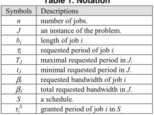
Essentially, a perfectly periodic schedule can be viewed as an infinite concatenation of a cycle. The related symbols and the corresponding descriptions are summarized in Table 1. In this paper, we assume that the granted period is greater than or equal to the required period for all jobs.

Table 1. Notation Symbols Descriptions

n number of jobs.

J an instance of the problem.

bi length of job i.

τi requested period of job i.

TJ maximal requested period in J.

tJ minimal requested period in J.

βi requested bandwidth of job i.

βJ total requested bandwidth in J.

S a schedule.

τiS granted period of job i in S.

To study the performance of perfectly periodic schedule, we evaluate the weighted average distortion, a popular measure first proposed in [2].

The weighted average distortion defined as

i S i n i

i J

S J

C β ττ

β

∑

=

1 AVE

) 1 , (

where the ratio of τiS / τi represents the distortion of job i and the weight of job i, βi, is the requested bandwidth. Obviously, the best case of distortion occurs when the granted period equals to the requested period.

2.2 Related Works

In the perfectly periodic scheduling problem, Bar-Noy [2] first suggested a binary tree-based algorithm to schedule requests with unit length. Later in [5, 6], Brakerski et. al. considered a more general problem for scheduling a set of requests with different lengths and periods. Recently, for the same problem in [5, 6], Patil and Garg [9] proposed a more efficient algorithm Adaptmin that schedules n jobs requests in O(nlogn) time.

In general, the requested period of each job may not be formed a power of two, algorithm Adaptmin rounds up all periods to the nearest power of two, i.e.,

⎡ ⁱ⎤

i τ

τ ^'=²^log² , and schedules the scaled jobs. Let the maximum period be T and the minimum period be t respectively. First, algorithm Adaptmin sorts the jobs in the nondecreasing order of requested periods and creates T/t intervals, each interval of length t slots, for a cycle. Next it processes the jobs in the nondecreasing order of requested periods. For job i, it scans the first

τ

_i'/

t

intervals and choose the first interval with most free slots. If the number of free slots is less than

τ

_i', the length of the interval is enlarged for job i. Since all intervals have the same length, all intervals are enlarged. Finally, the job is scheduled in all intervals that are at a multiple of

i'/

t τ

^.

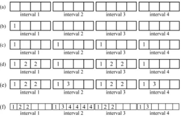
Figure 1 shows an instance of algorithm Adaptmin for J={(1, 8), (1, 4), (2, 7), (4, 13)}.

After rounding up all periods to the nearest power of two and sorting the requested periods, we have the scaled jobs J’={(1, 4), (2, 8), (1, 8), (4, 16)}, T = 16, and t = 4, as shown in Figure 1(a). Next find interval 1 with most free space and set the first job in interval 1, as shown in Figure 1(b). Then insert the first job into all intervals at a multiple of 1 interval away, as shown in Figure 1(c). Repeat the same procedure, Adaptmin schedules two slots for the second job in intervals 1 and 3 and one slot for the third job in intervals 2 and 4, as shown in Figure 1(d) and Figure 1(e). For the last job, since the free space of all intervals is less than the requested length of the fourth job, all intervals will be expanded so that the fourth job can be scheduled perfectly. In this case, the least number of slots to be expanded is two, so each interval will consist of six slots. Finally the ,

30

(12)

fourth job can be scheduled in interval 2, as shown in Figure 1(f).

Figure 1. An Example of Adpatmin.

Examining the last step in Figure 1, if we can schedule the second and third jobs both in intervals 1 and 3, the fourth job can be inserted into interval 2 just with one-slot expansion. On the other hand, since Adaptmin adjusts each period to its nearest power of two, the jobs with longer request period get higher distortion. Moreover, Adaptmin schedules jobs according to the nondecreasing order of periods and using the best-fit strategy to allocate the slots, then the jobs with long requested period and long requested length may result in interval expansion and bring more idle slots.

3. Algorithm GAS

In this section, we introduce a new algorithm called GAS for estimating more economic sizes of intervals instead of enlarging all periods to the nearest power of two. The algorithm is composed of three stages: the first stage is “Grouping” that divides jobs into lists according to requested periods;

the second stage is

“

^Adjusting” that determines the interval length to schedule all jobs tightly; and the third stage is “Scheduling” which schedules the jobs into intervals.

3.1 Procedure Group

For improving the average performance, the short-period jobs need to be served more often, thus we assign them with higher priority of scheduling.

But if two jobs have the same priority, the job with greater length is scheduled first. The aim of procedure Group is to classify the jobs into lists

according their periods and arrange the lists in the nonincreasing order of lengths. The detailed steps of procedure Group are shown in Figure 2. And Figure 3 gives an example for J = {(1,7), (8,39), (1,62), (1,64), (32,96), (2,122), (12,128)} processed by Procedure Group.

Procedure Group Input: Instance J Output: Lists L0,L1,…Lm-1

1. Sort J in nondecreasing order of periods and let B be the total length of all requested jobs.

2. Let the maximum period be T and the minimum period be t.

3. Create lists, says L0,L1,…Lm-1.

4. For all i, insert job i into list Lk where k = in nondecreasing order of periods and keep the list in nonincreasing order of length.

Figure 2. Procedure Group

Figure 3. An Example of Procedure Group

3.2 Procedure Adjust

The aim of procedure Adjust is to determine the length of schedule intervals, i.e., the minimum τiS of J.

For all jobs in list Lj, procedure Adjust tries to make an interval reservation to list Lj-1 by joining jobs in list Lj into a pseudo job and inserting it to list Lj-1 . The description of the procedure is given in Figure 4.

Procedure Adjust Input: Lists L0,L1,…Lm-1

Output: Lists L0,L1,…Lm-1 and length of interval l 1. For j = m-1 to 1

1.1 Distribute all jobs in list Lj into 2^j sets in noninecreasing order of lengths as evenly as possible.

1.2 For k = 1 to j

Join the (2k-1)th and (2k)th sets into a pseudo job and set the length of the

⎡ ⎤

⎡log₂τi/^B⎤−⎡log₂⎡^t/^B⎤⎤

⎡ ⎤

⎡^log2 ^/ ⎤−⎡^log2⎡ ⎤^/ ⎤+¹

= T B t B

m

31

(13)

pseudo job is the greater total length of two merged sets.

1.3 Record the scheduling order of jobs in pseudo jobs.

1.4 Insert 2^j-1pseudo jobs into list L_j-1 in noninecreasing order of lengths.

2. Let l be the sum the length of jobs in list L₀ 3. If ∃ job i (τi < 2^j× l), expand interval length to

l=l + max{⎡(τi – (2^j× l)) / 2^j⎤}.

Figure 4. Procedure Adjust

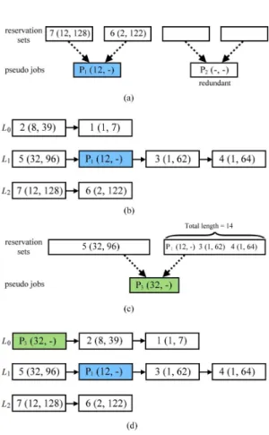
Figure 5. An Example of Procedure Adjust For any list Lj, we distribute all jobs in list Lj into 2^j sets in noninecreasing order of lengths as evenly as possible. Next join two consecutive sets into a pseudo job and set the length of the pseudo job is the greater total length of two merged jobs. Then insert the 2^j-1pseudo jobs into list L_j-1 in noninecreasing order of lengths. We do this process for lists in the order of Lm-1, Lm-2, …,L1. Let l be the total length of jobs in list L₀. Finally, procedure Adjust scans all jobs and adjusts the maximum interval. The size of the maximum interval is extended to l = l + max{⎡(τi – (2^j× l)) / 2^j⎤ } for all job i with period

longer than 2^j× l slots where job i is in Lj.

An example of procedure Adjust is shown in Figure 5. Note that the interval length l = 41 obtained by the total length of jobs in L₀. But, since the request period of job 5 is longer than l and job 5 is in L₁, we extend interval to l = 41 + ⎡(96-2¹×41) / 2⎤ = 48, i.e.

each interval is extended four slots.

3.3 Procedure Schedule

The aim of procedure Schedule is to schedule all jobs according to the lists produced by procedure Adjust. The description of the procedure is given in Figure 6. The procedure first round all periods by τiS = 2^j × l, where job i is in the list Lj. Let the maximum scheduled period T^S = max{τ_i^S} and minimum scheduled period t^S = min{τ_i^S}. Next we create T^S / t^S intervals with equal length l. To schedule all jobs into intervals, the algorithm schedule jobs from L₀ to L_m-1 and in decreasing order of length. At the begining of scheduling, all of the space of interval can be scheduled for list L0. But for list L_j(j≠0), the intervals to be scheduled is constrained to the reservation by pseudo jobs in list Lj-1. Then schedule jobs of list Lj into constrained intervals in nonincreasing order of length. For each job, find an interval with the position that belongs for current examined job in first τ_i^S / t^S constrained intervals. Insert the job in the interval and in the intervals at a multiple of τiS / t^S away.

Procedure Schedule

Input: Lists L0,L1,…Lm-1 and length of interval l Output: A schedule S.

1. For all jobs (including pseudo jobs), round all job periods to τ_i^S = 2^j× l, if job i is in the list Lj. 2. Let T^S = max{τiS} and t^S = min{τiS}.

3. Produce T^S / t^S intervals with equal length l.

4. Insert all jobs in L₀ into all intervals directly.

5. Let j = 1 and set the intervals for pseudo job in L0 as constrained interval.

6. Schedule jobs of list L_j into constrained intervals in nonincreasing order of length. Search first τ_i^S / t^S constrained intervals and insert jobs into appropriate positions according to the related scheduling record.

32

(14)

7. Insert the job into all intervals at a multiple of

S iS/t

τ intervals away.

8. Set j = j+1 and let the constrained intervals in the next iteration be the scheduled intervals for pseudo jobs. Repeat step 6 to 8 until j = m.

Figure 6. Procedure Schedule

Figure 7. An Example of Schedule

Continuing the example in Figure 5, the scheduling for the instance is shown in Figure 7.

From procedure Adjust, we have l=48. Procedure Schedule first rounds all periods, then define T^S= 192 and t^S= 48 and create four (192 / 48 = 4) intervals with length 48, as shown in Figure 7(a). The jobs in L0 is scheduled first. Consider the pseudo job P₃ of L₀. The pseudo job P₃ in L₀ is inserted into all intervals directly, as shown in Figure 7(b). The other jobs in L₀ are scheduled similarly, shown in Figure 7(c). For the next list L1, the procedure scans the first two constrained intervals, and schedules jobs into appropriate positions according to the related scheduling record. Then the job is allocated into all intervals at a multiple of two intervals away, as shown as Figure 7(d). Process the other lists in the same way. Finally the schedule S is given in Figure 7(e).

4. Simulations

In this section, we compare the performances of algorithm Adaptmin and algorithm GAS based on the average efficiency of the schedule and time complexity. The simulations are performed using C language with IBM PC and the simulation data is generated by the approach proposed in [9].

To compare the efficiency of algorithms, an

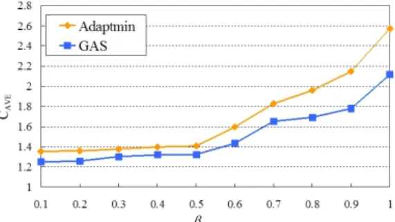
approach for producing simulation data is proposed in [9]. The simulation results are shown in Figures 8-10. The comparison of performance CAVE of two algorithms with the maximum period τmax= 128 is shown in Figure 8. As expected, when the requested bandwidth β⁽⁰≤ β≤ 1) is high, algorithm GAS can arrange the jobs into more compact intervals to reduce the number of idle slots. More specifically, for the cases of β > 0.5, our approach can improve efficiency from 10% to 20%. Even in the case of β⁼ 1, from Figure 9, the average efficiency CAVE of GAS is better than that of Adaptmin. The comparison of time complexity is given in Figure 10. The result shows that algorithm GAS performs better than algorithm Adaptmin.

Figure 8. Performances of Adaptmin and GAS with τmax = 128.

Figure 9. Performances of Adaptmin and GAS with β = 1.

Figure 10. Complexity Comparison of Adaptmin and GAS.

33

(15)

5. Conclusions

In this paper, we considered the perfectly periodic scheduling problem for the client requests with different requested periods and various requested lengths. Algorithm GAS we proposed is based on the strategy which balances the effects of the request periods and the request lengths. Our simulation results show that algorithm GAS performs well when the total requested bandwidth is high and the range variance of requested period is large.

6. References

[1] S. Acharya, R. Alonso, M. Franklin and S. Zdonik, Broadcast disks: data management for asymmetric communication environments, Proceeding of ACM SIGMOD, Mar. 1995, pp. 199-210.

[2] A. Bar-Noy, V. Dreizin and B. Patt-Shamir, Efficient periodic scheduling by trees, Proc. 21^st Annual Joint Conf.

of the IEEE Computer and Communications Societies, Vol.

2, June 2002, pp.791-800.

[3] A. Bar-Noy, B. Randeep, J. Naor and B. Schieber, Minimizing service and operation cost of periodic scheduling, Proceeding of the 9^th Annual ACM-SIAN Symposium on Discrete Algorithms, 1998, pp. 11-20.

[4] Bluetooth technical specifications, version 1.1. from http://www.bluetooth.com/, Feb. 2001.

[5] Z. Brakerski, A. Nisgav and B. Patt-Shamir, General perfectly periodic scheduling, 21^st Annual Symp. on Principles of Distributed Computing, 2002, pp. 163-172.

[6] Z. Brakerski, A. Nisgav and B. Patt-Shamir, General perfectly periodic scheduling, Algorithmica, 45(2), 2006, pp. 183-208.

[7] N. Dhanakoti, S. Gopalan and V. Sridhar, Perfectly periodic scheduling for fault avoidance in IEEE 802.11e in the context of home networks, 14^th Annual IEEE Internat.

Symp. on Software Reliability Engineering, November 17-20, 2003.

[8] T. Imielinski, S. Viswanathan and B. Badrinath, Data on air: organization and access, IEEE Transactions on Knowledge and Data Engineering, 9(3), Jun. 1997, pp.

353-372.

[9] S. Patil and V. K. Garg, Adaptive general perfectly periodic scheduling, Information Processing Letters, 98(3), 2006, pp. 107-114.

[10] W. C. Peng, J. L. Huang and M. S. Chen, Dynamic leveling: adaptive data broadcasting in a mobile computing

environment, Mobile Networks and Applications, 8(4), 2003, pp 355-364.

[11] C. J. Su and L. Tassiulas, Joint broadcast scheduling and user’s cache management for efficient information delivery, Proceedings of the 4^th ACM/IEEE International Conference of Mobile Computing and Networking, Oct.

1998, pp. 33-42.

[12] J. Xu, X. Tang and W.-C. Lee, Time-critical on-demand data broadcast: algorithms, analysis, and performance evaluation, IEEE Transactions on parallel and distributed systems, 17(1), 2006, pp. 3-14.

34