ABSTRACT
The displacement of a rigid body from one position to the other can be described by using a screw axis, and the screw axis degenerates to a point, called pole, in a planar displacement. All possible displacement screw axes of a certain link (usually the coupler) of a one-degree-of-freedom spatial linkage constitute a ruled surface, called screw surface. The planar degeneration of a screw surface is a planar curve, called rotation curve. This proposed project is a two-year project. In the first year of the project, we propose to investigate the rotation curves of planar four-bar and six-bar linkages. In the second year, we plan to investigate the screw surfaces of spatial four-bar linkages. Rotation curves and screw surfaces can be thought of as the description of workspaces of one-degree-of-freedom linkages. They are significant in synthesizing linkages and in evaluating the performances of linkages.
In the first year of this project, we investigated the rotation curves of all types of planar four-bar linkages. By using a novel technique, we derived the analytical expressions of these rotation curves. Furthermore, we built a computerized atlas of the rotation curves, to be used as a reference in mechanism design. In the second year of this project, we extended the investigation to spatial four-bar linkages to derive the analytical expressions of their screw surfaces. Furthermore, we studied the properties of the screw surfaces, with the aid of three-dimensional visualizations on a computer.
Most of the proposed tasks, except for some primitive studies in planar four-bar linkages, are novel in the research and development of mechanisms. The investigation of the screw surfaces of spatial linkages is particularly creative. The result presented here is not only of theoretical importance in mechanism theory but also practical in the design and evaluation of linkages.
2
ABSTRACT
3
1
5
1.1
5
1.2
4R
5
1.3
10
1.4
12
1.5
15
1.6
16
1.7
17
2
RPRP
(
)
18
2.1
Introduction
18
2.2
Two Types of Spatial RPRP Linkages
19
2.3
The Intersection of Finite Screw Systems
1
2.4
The Screw System Associated with the Screw Surface
of the RPRP Linkage
23
2.5
The 3-Systems Associated with PR and RP Dyads
23
2.6
The Intersection of Screw Systems for the Folded
RPRP Linkage
25
2.7
The Intersection of Screw Systems for the Unfolded
RPRP Linkage
26
2.8
Numerical Example
27
2.9
Conclusion
28
2.10 References
29
3
31
32
Lohse
1.1
Σ0 Σ1 P01 0 Σ Σ1 Σ2 P02 0 Σ Σ2 0 Σ 1 1 1955 Lohse[1][2] Grashof 1967 Veldkamp[3] 4R 1973 Popa Unteanu[4] Manolescu Popa[5] 1975 Manolescu Popa[6] 4RManolescu Popa Manolescu
Popa 4R
1.2
4R
2 4R A0B0 P A0B0B1A1 A0B0B2A2 2 1 2 1PA BPB A =∠ ∠ , PA1=PA2, PB1=PB2, ∠A0PA1=∠B0PB1 ∠A0PA1−∠B0PB1 =π 1 1 0 0PB APB A =∠ ∠ ∠A0PB0−∠A1PB1 =π (1)(a) (b) 3 4R r1 r2 r3 r4 A0B0B1A1 2 X θ2 4 X θ4 (1) ∠A1PB1 ∠A0PB0 φ 4 φ=α4−α2
(
)
2 4 2 4 2 4 1 α α α α α α φ tan tan tan tan tan tan + − = − = (2) P( )
x,y x y 2= α tan , 1 4 r x y − = α tan (3) (2) 2 1 1 1 1 y r x x y r x xy x y r x y 1 x y r x y + − − − = ⋅ − + − − = ) ( ) ( tanφ (4) 5 X′ X φ=β4−β2(
)
2 4 2 4 2 4 1 β β ββ β β φ tan tan tan tan tan tan + − = − = (5) 2 β tan tanβ4 2 2 2 2 2 c r x s r y θθ β − − = tan , tan(
)
4 4 1 4 4 4 c r r x s r y θ θ β + − − = (5)(
)
(
)
2 2 2 2 4 4 1 4 4 2 2 2 2 4 4 1 4 4 c r x s r y c r r x s r y 1 c r x s r y c r r x s r y θθ θ θ θ θ θ θ φ − − ⋅ + − − + − − − + − − = tan(
(
)(
)
) (
) (
[
)
]
[
1 4 4]
(
2 2) (
4 4)(
2 2)
4 4 1 2 2 2 2 4 4 s r y s r y c r x c r r x c r r x s r y c r x s r y θ θ θ θ θ θ θ θ − − + − + − + − − − − − = (6) + − + ± = − C B C B A A 2 2 2 2 1 4 tan θ , 2 A=sinθ , 2 1 2 r r B=cosθ − , 4 2 2 4 2 3 2 2 2 1 2 4 1 r r 2 r r r r r r C=− cosθ + + − + (4) (6)(
) (
) (
)
[
]
[
4 4]
(
2 2) (
2 2) (
1 4 4)
1 2 1 1 4 4 2 2 4 4 2 2 ( ) ( ) ( ) ( ) y r s x r c y r s x r r c xy x r y x x r y x r r c x r c y r s y r sθ
θ
θ
θ
θ
θ
θ
θ
− − − − − + − − = − + − + − + − − 4R(
)
(
)
(
)
(
)
(
)
(
)
(
)
(
r rc rrrc c rrrs s)
y 0 x s c r r r s r r c s r r r xy c r r 2 y c s r r s c r r s r r x c s r r s r r s r r 2 s c r r xy s r s r y x c r c r y c r c r x s r s r 4 2 4 2 1 4 2 4 2 1 2 2 2 1 4 2 4 2 1 2 2 2 1 4 2 4 2 1 2 2 1 2 4 2 4 2 4 2 4 2 4 4 1 2 4 2 4 2 4 4 1 2 2 1 4 2 4 2 2 4 4 2 2 2 2 2 4 4 3 2 2 4 4 3 4 4 2 2 = + + − − + + + − + + − − − + − + − + − + − θ θ θ θ θ θ θ θ θ θ θ θ θ θ θ θ θ θ θ θ θ θ θ θ θ θ θ θ θ θ (7) 3 4R 4 4R5 4R 6 8 Grashof 4R 1 8(d) Huang[7] Bennett Bennett 8(d)
(
r1,r2,r3,r4,θ2)
=(
7,3,4,5,60)
6 Non-Grashof(
s+l> p+q)
(
r1,r2,r3,r4,θ2)
=(
2,4,5,6,60)
(
r1,r2,r3,r4,θ2)
=(
4,2,5,6,60)
(
r1,r2,r3,r4,θ2)
=(
5,4,2,6,60)
(a) (b) (c) 7 Grashof(
s+l< p+q)
(
r1,r2,r3,r4,θ2)
=(
6,3,4,5,30)
(
r1,r2,r3,r4,θ2)
=(
2,2,4,4,60)
(a) (b)(
r1,r2,r3,r4,θ2)
=(
2,4,2,4,60)
(
r1,r2,r3,r4,θ2)
=(
2,4,2,4,30)
(c) (d)(
r1,r2,r3,r4,θ2)
=(
4,4,4,4,60)
(e) 8(
s+l= p+q)
1 4R a.Non-Grashof l+s> p+q b. c. d. q p s l+ < + e. l+s= p+q i) l≠s≠ p≠q (rational cubic) ii) p l= ;s=q iii) l= p;s=q iv) l=s= p=q l s p q1.3
9 r2 r3 X X e A0B0B1A1 2 X θ2 A1B1 A2B2 P PA0 A1A2 0 PB B1B2 X B0 B0 φ = ∠ = ∠A0PB0 A1PB1 P( )
x,y PB0 X A0PB0 y x = φ tan (8) 10 X′ X φ=β4−β2(
)
2 4 2 4 2 4 1 β β β β β β φ tan tan tan tan tan tan + − = − = (9) 2 2 2 2 2 c r x s r y θ θ β − − = tan L x e y 4 − − = β tan(
)
2 2 2 2 3 2 2 r r e r L= cosθ + − sinθ − (9) 2 2 2 2 2 2 2 2 r x r y L x e y 1 r x r y L x e y θ θ θ θ φ cos sin cos sin tan − − ⋅ − − + − − − − − =(
)(
) (
)(
)
(
)(
2 2) (
)(
2 2)
2 2 2 2 r y e y r x L x r y L x r x e y θ θ θ θ sin cos sin cos − − + − − − − − − − = (10) (8) (10)(
)(
) (
)(
)
(
)(
2 2) (
)(
2 2)
2 2 2 2 r y e y r x L x r y L x r x e y y x θ θ θ θ sin cos sin cos − − + − − − − − − − =(
)
(
)
(
)
(
Lr er)
y 0 x er Lr xy r 2 y r L x r L xy x 2 2 2 2 2 2 2 2 2 2 2 2 2 2 2 2 2 3 = − + + + − − − + − + cos sin sin cos sin cos cos θ θ θ θ θ θ θ (11) 910 11 12 2
(
r2,r3,e,θ2)
=(
6,6,0,30)
(
r2,r3,e,θ2)
=(
4,6,0,30)
11(
r2,r3,e,θ2)
=(
4,6,1,30)
(
r2,r3,e,θ2)
=(
4,6,2,30)
(
r2,r3,e,θ2)
=(
4,6,3,30)
122 max min r r = max min r r ≠ max min e r r + < max min e r r + = max min e r r + > min r rmax r2 r3 e
1.4
13 A0B0B1A1 2 X θ2 A1B1 A2B2 P PC1 PC2 A1B1 A2B2 P B0 A1B1 A2B2 C2 C1 14 4 2 0 1 0B BB r B = = 1 PC PC2 A1B1 A2B2 A1B1 A2B2 C C B B C B B0 1 =∠ 0 2 = = − ∠ CB B0 1= ∠ , ∠B0CB2 = α δ sin sin C B r4 = 0 , α ξ sin sin C B r4 = 0 (12) (12) sinδ =sinξ δ ≠ξ ξ =π−δ B0C ∠A1CB2 P A1B1 A2B2 C2 C1 PC1=PC2 2 C PC C PC1 =∠ 2 = ∠ PC1C PC2C ∠PCC1=∠PCC2 PC ∠A2CB1 1314 B0C ∠A1CB2 PC ∠A2CB1 PB0 A1B1 A2B2 C φ = ∠ = ∠A0PB0 A1PC1 P
( )
x,y A0PB0 2 1 1 1 1 y r x x y r x xy x y r x y 1 x y r x y + − − − = ⋅ − + − − = ) ( ) ( tanφ (13) 15 X′ X φ=β4−β2(
)
2 4 2 4 2 4 1 β β β β β β φ tan tan tan tan tan tan + − = − = (14) 2 2 2 2 2 c r x s r y θ θ β − − = tan(
4 2)
4 β γ θ π β =tan =tan + − tan (14)(
)
(
)
2 2 2 2 4 2 2 2 2 4 c r x s r y 2 1 c r x s r y 2 θ θ π θ γ θθ π θ γ φ − − ⋅ − + + −− − − + = tan tan tan(
(
)
(
)(
) (
)(
)
)
2 2 4 2 2 2 2 2 2 4 s r y 2 c r x s r y c r x 2 θ π θ γ θ θ θ π θ γ − − + + − − − − − + = tan tan (15) − ± − = − S 2 SU 4 T T 2 2 1 4 tan θ , S=R−Q, P 2 T = , U=Q+R,(
θ)
γ γθ sin cos cos
sin 2 2 2 1 2 r r r P= + − ,
(
θ)
γ γθ cos cos sin
sin 2 2 2 1 2 r r r Q=− + − , γ sin 4 r R=− (13) (15)
(
)(
) (
)
(
2 2)
(
4)(
2 2)
2 2 2 2 4 2 1 1 s r y 2 c r x s r y c r x 2 y r x x y r x xy θ π θ γ θθ π θ θ γ − − + + − − − − − + = + − − − tan tan ) ( ) ( µ π θ γ + 4− 2=(
)
(
)
(
)
(
rrc rrs)
y 0 x s r r c r r y r c r s r x r c r s r xy y x y x 2 2 1 2 2 1 2 2 1 2 2 1 2 1 2 2 2 2 2 1 2 2 2 2 2 2 3 3 = + + − + − − + − − + ⋅ + − − ⋅ tan tan tan tan tan tan tan tan µ θ θ θ µ θ µ µ θ θ µ µ θ θ µ µ (16) 15 16 (16) 90 = γ 4 e r4sinγ e 3(
, , , ,r r r1 2 4 γ θ =2)
(
6,6,0,90 ,60)
( , , , ,r r r1 2 4 γ θ2)=(
6,4,0,90 ,60)
( , , , ,r r r1 2 4γ θ2)=( 6,4,1,90 ,60) ( , , , ,r r r1 2 4γ θ2)=(
6, 4, 2,90 ,60)
(r1,r2,r4,γ,θ2)= (6,4,3,90 ,60 ) 163 max min r r = 0 r4sinγ = max min r r ≠ max min e r r + < max min e r r + = 0 r4sinγ ≠ max min e r r + > min r rmax r1 r2 e=r4sinγ
1.5
17 ψ L2 r3 P( )
x,y ∠A0PB0=∠A1PB1=φ φ=π−ψ 17(
)
ψ ψ ψ ψ ψ π cos sin cos sin tan 2 2 4 2 2 4 L x L y L x y 1 L x L y L x y − − ⋅ − + − − − − = − (17)(
)
2 2 2 3 2 4 L r L L = cosψ + − sinψ(
)
2 2(
)
2 2 2 2 2 3 2 3 2 2 2 3cos sin cot sin sin
2 2 csc 2 L r L r L L x y r
ψ
ψ
ψ
ψ
ψ
ψ
+ − − − − + + = (18)18 (Moving Polode) 19 AB Ca Cc (Gardan) Ca P0 Ca C CO AC BC Ca O
(
L2,r3,ψ)
=(
5,4,50)
18 191.6
4R1.7
[1] Lohse, P., “Polortkurven als Hilfsmittel zur Konstruktion von Gelenkgetrieben,” Z. angew.
Math. Mech., Volume 38, No. 1/2 (1958).
[2] Lohse, P., Getriebesynthese, Springer-Verlag, Berlin (1975).
[3] Veldkamp, G. R., “Rotation Curves,” Journal of Mechanism, Vol. 2, pp. 147-156 (1967).
[4] Popa, Gh. C. and Unteanu, C. E., “Sinteza Tripositionala pe Baza Curbelor ( n k
p ),” Proceedings of the IFToMM International Symposium on Linkages and Computer Design Methods, Bucharest, Romania, June 7-13, Volume A, Paper 39, pp. 515-527 (1973).
[5] Manolescu, N. I., and Popa, Gh. C., “Sinteza Patru si Cinci-Positionala pe Baza Curbelor
( n k
p ),” Proceedings of the IFToMM International Symposium on Linkages and Computer Design Methods, Bucharest, Romania, June 7-13, Volume A, Paper A-31, pp. 409-421 (1973). [6] Manolescu, N. I., and Popa, Gh. C., “The Equations of the ( n
k
p ) Curves of the Planar Four-Bar Kinematic Chains,” Avtomaticheskaya Svarka, The 4th World Congress on the Theory of Mach and Mech, pp. 665-669 (1975).
[7] Huang, C., “The Cylindroid Associated with Finite Motions of the Bennett Mechanism,”
Journal of Mechanical Design, Trans. ASME, Vol.119, pp.521-524 (1994). [8] Beyer, R., Kinematische Getriebesynthese, Springer-Verlag, Berlin (1953).
[9] Erdman, A. G., and Sandor, G. N., Advanced Mechanism Design: Analysis and Synthesis, Vol.
2, Prentice-Hall, New Jersey (1984).
[10] Norton, R. L., Design of Machinery, McGraw-Hill, Inc., New York (1992).
[11]
RPRP
Linear Property of the Screw Surface of the Spatial RPRP Linkage
This paper investigates the screw surface of the RPRP linkage, an overconstrained linkage with mobility one. The screw surface is a ruled surface containing screws for displacing the coupler of the RPRP linkage from one reference position to all reachable positions. In this paper, two types of RPRP linkages, in folded and unfolded forms, are constructed by using hexahedrons in accordance with Delassus’ criteria. It is shown that the screw surfaces of both types of RPRP linkages can be represented by screw systems of the second order. These novel finite screw systems are obtained by intersecting two 3-systems corresponding to the finite displacements of the RP and PR dyads. The intersection of finite screw systems is conducted by employing the intersection operation of vector subspaces of the six-dimensional vector space.
2.1 Introduction
Delassus [1] derived all the four-bar linkages composed of lower pairs with connectivity one. If one considers only revolute (R) and prismatic (P) joints, there are three spatial overconstrained linkages with connectivity sum four: the spatial 4P, the spatial 4R, and the spatial RPRP linkages. The motion of the spatial 4P is obvious, and the spatial 4R linkage is the famous Bennett mechanism [2]. However, the motion of the RPRP has drawn less research attention. This paper investigates the finite motion of the RPRP linkage, with an emphasis on the linear property of its screw surface. A screw surface[3], analogous to the rotation curve [4, 5] of a two-dimensional motion, is a ruled surface containing screws for finite displacements that bring a rigid body, in one-degree-of-freedom spatial motion, from one reference position to all possible positions. The screw surfaces of overconstrained linkages are of special interest here because they can form screw systems.
Until recently, most research in overconstrained linkages has focused on the mobility and instantaneous kinematic geometry of the linkages. Then Huang [6] demonstrated that the screw surface of the Bennett mechanism formed a 2-system. This 2-system was obtained by intersecting two 3-systems [7], corresponding to the RR dyads forming the Bennett mechanism. Remarkably, this linear property of the Bennett mechanism can also be found in most Bennett-based mechanisms [8, 9]. The discovery of finite screw systems is relatively novel in kinematic geometry because finite kinematics, unlike instantaneous kinematics, had been considered to be nonlinear. In addition to their theoretical importance in kinematic geometry, finite screw systems can substantially simplify the analysis and synthesis of spatial linkages [10, 11].
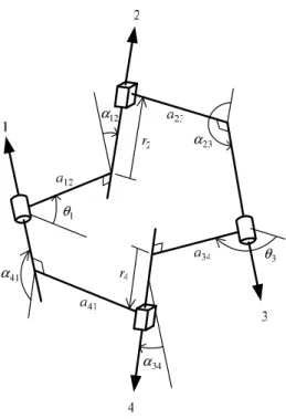
12 α 23 α 34 α 41 α θ3 1 θ
Fig. 1 General Arrangement of the RPRP Linkage
In searching for more finite screw systems, it is noteworthy that there are analogies between the Bennett and the RPRP linkages: they are both of connectivity sum four, but possess one degree of freedom, and the dyads forming the linkages, the RR and RP dyads, both possess linear properties. It is natural to conclude that the screw surface of the RPRP linkage might also possess linear properties [12]. This paper successfully extends the theories and methods developed for the Bennett mechanism to unveil the 2-system associated with the RPRP linkage.
The organization of this paper is as follows: first, two types of RPRP linkages are constructed based on Delassus’ criteria, and the loop closure equations for both types of RPRP linkage are derived. Second, the concepts of finite screw systems and their intersections are discussed. Third, the screw surface of the RPRP linkage is shown to be a 2-system by intersecting the corresponding dyad screw systems. Finally, a numerical example is used to illustrate the linear property of the screw surface and to validate the derived 2-system.
2.2 Two Types of Spatial RPRP Linkages
Figure 1 shows the schematic drawing of a spatial RPRP linkage, of which joints 1 and 3 are revolute, while joints 2 and 4 are prismatic. The offset distance and twist angle between two adjacent joint axes are denoted by aij and αij, respectively. The translational distance and joint angle
between the two incident normals of a joint axis are denoted by ri and θi, respectively. The link
in general, it is not mobile. However, this linkage can possess mobility one if the revolute joints are parallel and the directions of the prismatic joints are symmetric with respect to the plane containing the revolute axes [1, 13, 14].
Fig. 2 The Folded RPRP Linkage Fig. 3 The Unfolded RPRP Linkage
Following Delassus’ criteria for the RPRP linkage, we can obtain two types of RPRP linkages, in folded and unfolded forms, which differ from each other in the twist angles. Figures 2 and 3 show the construction of these two types of linkages by using different hexahedrons. In what follows, we
describe the geometric constraints of both types of linkages and derive their loop closure equations. In an RPRP linkage, the variables are the joint angles of the revolute joints, θ1 and θ3, and the
translational distances of the prismatic joints, r2 and r4. Since the mobility of the RPRP linkage is
one, three scalar equations (the loop closure equations of the linkage) must be obtained. According to the mobility criteria of the linkage, the geometric constraints of the folded RPRP linkages can be obtained as follows: (offset distances) a12 =a41, a23 =a34, a12// a23, a34// a41; (twist angles) α =12 α34,
41 23 α
α = , α12+α23=π; (translational distances) r1= r3 =0; (joint angles) θ2 =θ4 =0.
In order to obtain the loop closure equations, as shown in Figure 4, we observe the linkage from the direction of the revolute joint axes. From this top view of the folded RPRP linkage, we obtain the following three closure equations:
1 3 π θ θ = + 4 2 r r = 12 2 1 23 12 )tan 2 sin (a +a θ =r α
The geometric constraints of the unfolded RPRP linkage are identical to those of the folded RPRP linkage except for the twist angles: α =12 α23; α =34 α41; α12+α34=π.
Similarly, in order to obtain the loop closure equations, as shown in Figure 5, we observe the linkage from the direction of the revolute joint axes. From this top view of the unfolded RPRP linkage, we obtain the following three closure equations:
1 3 π θ θ = − 4 2 r r =
(
a12−a23)
tanθ21 =r2sinα12 3 θ 3 34 a 23 a 4 r 2 r 2 4 12 a 41 a 1 1 θ 12 a 3 θ a23 34 a 41 a 1 θFig. 4 Top View of the Folded RPRP Linkage Fig. 5 Top View of the Unfolded RPRP Linkage
2.3 The Intersection of Finite Screw Systems
In this paper, we are primarily concerned with the screw surface of the coupler of the RPRP linkage. The screw surface of a spatial linkage is the ruled surface that contains all screws for displacing the coupler from one reference position to all possible positions. The screw surface is usually obtained by solving nonlinear equations [3]. However, if the finite motion of both the dyads forming the linkage can be represented by using screw systems, the screw surface can be obtained by the intersection of corresponding finite screw systems, As a result, the obtained screw surface can also be represented by a screw system. In what follows, we review the fundamental concepts regarding finite screw systems and their intersections.
A screw is mathematically defined as a line with an associated pitch, and it can be treated as a vector in a six-dimensional vector space. Screw coordinates, S=(s,ˆso), of a screw are composed of two Cartesian vectors, one of which is the direction vector, sˆ, of the line (screw axis), and the other is the moment vector, so. The moment vector is defined as: so =r×sˆ+psˆ, where r is the position
vector of any point on the line, and p is the pitch of the screw. Since the magnitude of the direction vector is immaterial, we can normalize the direction vector to obtain a unit screw. In this paper, we use the symbol ∧ above a boldface letter to denote a unit vector or a unit screw.
When a set of screws are closed under addition and scalar multiplication, they form a screw system. A screw system of the nth order (an n-system) contains ∞n−1 screws and corresponds to a
vector subspace of rank n. It is well known that the instantaneous motion of a rigid body with N DOF can be generally described by an N-system [15]. Finite displacement screws normally do not form screw systems. Parkin [16] unveiled a new definition of pitch for a finite displacement screw, in which pitch was the ratio of one-half the translation to the tangent of one-half the rotation. If Parkin’s definition of pitch is used, finite displacement screws can form screw systems. Nevertheless, unlike in instantaneous motion, the finite displacement of a rigid body with N DOF can be generally described by an (N+1)-system if the corresponding finite screw system exists. The statement is true if we exclude the case in which the finite motion is generated by a single kinematic joint.
It has been demonstrated that the operations of vector subspaces can be employed in finite kinematic analysis of mechanisms [6, 9]; however, special attention should be paid because finite screw systems are in fact not vector subspaces. Instead, a finite screw system corresponds to the projective space associated with the vector subspace spanned by the basis screws of the screw system [17]. In a projective space, vectors that differ from one another only in magnitude are considered to be equivalent and are represented by a homogeneous vector.
In addition to the theoretical importance of finite screw systems, one of the most attractive advantages is that kinematic analysis can be substantially simplified by using the vector subspace operations of screw systems. For example, the coupler motion of the Bennett mechanism is compatible to both RR dyads forming the mechanism and is obtained by the intersection of vector subspaces corresponding to the RR dyads [6]. The application of intersections of screw systems in instantaneous kinematics is well known; however, the concept of employing the intersection of finite screw systems in finite kinematic analysis is relatively new.
Since finite screw systems correspond to projective spaces, the intersection of finite screw systems becomes that of projective spaces. The following proposition allows us to conduct the intersection: the projective space associated with the intersection of some vector subspaces of a vector space is the intersection of the projectivizations of these subspaces [18-20]. For example, to study the finite motion of one link of the RPRP linkage (the coupler link) with respect to its opposite link (the ground link), the finite motion of the coupler of the RPRP linkage must be
compatible with the RP and PR dyads. Namely, the coupler finite motion can be obtained by the intersection of the screw systems (vector subspaces) associated with both dyads. It is known that the intersection of two vector subspaces, if not a zero vector, must be a vector subspace. In general, the intersection of two finite screw systems is a zero vector. However, since the mobility of the overconstrained RPRP linkage is one, the intersection of the finite screw systems of the dyads must contain ∞1 screws. Therefore, the intersection must be a vector subspace of rank 2, which
corresponds to a 2-system.
In practice, we can utilize the operation of orthogonal complements of vector subspaces to calculate the intersection of two screw systems. When calculating the orthogonal complement to a screw system in radial (or axial) coordinates, we obtain its orthogonal complement in axial (or radial) coordinates. Two consecutive orthogonal complement operations are required in obtaining the intersection of two screw systems [6, 18-20]. Therefore, we obtain the intersection of two screw systems in the same type (radial or axial) of coordinates.
2.4 The Screw System Associated with the Screw Surface of the RPRP Linkage
In this section, the 3-systems associated with the finite displacements of the RP and PR dyads are summarized [21]. Joint screw coordinates for both types of RPRP linkages are determined in appropriate coordinate systems. Then the analytical expression for the 2-system associated with each type of the RPRP linkage is derived by the intersection of dyad screw systems.
2.5 The 3-Systems Associated with PR and RP Dyads
As shown in Figure 6, a rigid body (denoted by Σ) undergoes finite displacements accomplished by a PR dyad. The motion of Σ can be decomposed into two successive displacements. First, the pure rotation of the R joint takes the body from its original position to an intermediate position. SR
denotes the screw for the motion of the R joint, and θ is the rotation of the R joint. Second, the pure translation of the P joint takes the body from the intermediate position to its final position. SP
denotes the screw for the motion of the P joint, and t is the translation of the P joint. Note that the location of the pure translational screw SP is immaterial, and only its direction is crucial. We can
thus locate the axis of SP anywhere in space in such a way that it is parallel to the axis of the P joint.
The resultant displacement screw of these two successive displacements is represented by a screw, denoted by SPR.
R P P R PR t t S S S S S = + + × 2 2 tan 2 θ
As a result, SPR belongs to a 3-system, of which SR, SP, and SP×SR are a set of basis screws. Here R
P S
S × denotes the screw product [22-24] of SP and SR. Note that the magnitude (intensity) of the
screw SPR, obtained from the equation above, is irrelevant, and we are only concerned with its unit
screw. In terms of linear algebra, SPR belongs to the projective space associated with the vector
subspace spanned by SR, SP, and SP×SR.
R P S S × P S ΣΣΣΣ R S
Fig. 6 Basis Screws of the PR Dyad Displacements
R S P S P R S S × ΣΣΣΣ
Fig. 7 Basis Screws of the RP Dyad Displacements
Similarly, for an RP dyad, as shown in Figure 7, the resultant finite displacement screw SRP can
P R R P RP t t S S S S S = + + × 2 2 tan 2 θ
Again, SRP belongs to a 3-system, of which SR, SP, and SR×SP are a set of basis screws.
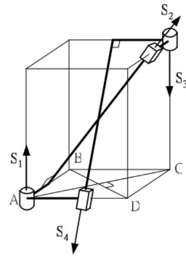
2.6 The Intersection of Screw Systems for the Folded RPRP Linkage
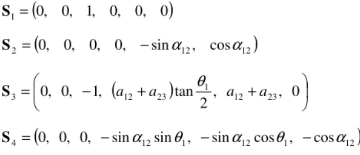
Figure 8 shows the schematic drawing of a folded RPRP linkage. The axis of joint 1 is taken as the Z-axis of the coordinate system, and the X-axis is coincident with the common perpendicular of the axes of joints 1 and 2. The screw coordinates of the joints are obtained as follows:
(
0, 0, 1, 0, 0, 0)
1= S(
12 12)
2= 0, 0, 0, 0, −sinα , cosα S(
+)
+ − = , , 0 2 tan , 1 , 0 , 0 12 23 1 12 23 3 a a θ a a S(
12 1 12 1 12)
4= 0, 0, 0, −sinα sinθ, −sinα cosθ , −cosα
S
Let link 12 be the fixed link. We are concerned with the finite displacement of link 34 with respect to link 12. The displacement of link 34 must be compatible with the dyad formed by joints 2 and 3 (the PR dyad) and that formed by joints 4 and 1 (the RP dyad). According to previous discussions, all possible finite displacement screws of the PR dyad belong to a 3-system, of which
2
S , S3, and S ×2 S3 are a set of basis screws, where
(
0, 0, 0, sin 12, 0, 0)
3 2×S = α S 2 S 3 S 1 S 4 S X Y ZSimilarly, all possible finite displacement screws of the RP dyad belong to a 3-system, of which
1
S , S4, and S ×1 S4are a set of basis screws, where
(
0, 0, 0, cos 1sin 12, sin 12sin 1, 0)
4
1×S = − θ α α θ
S
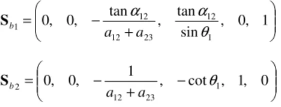
Then the intersection of the two finite 3-systesms associated with the PR and RP dyads is calculated by employing the intersection operation of vector subspaces [6, 18-20]. The intersection is a 2-system, of which a set of basis screws are obtained as follows:
+ − = , 0, 1 sin tan , tan , 0 , 0 1 12 23 12 12 1 a αa αθ b S − + − = 0, 0, 1 , cot 1, 1, 0 23 12 2 a a θ b S
These two basis screws are illustrated in Figure 9. They are both parallel to the Z-axis. It can be shown that the screw system is of the fourth special 2-system [15].
2.7 The Intersection of Screw Systems for the Unfolded RPRP Linkage
Figure 10 shows the schematic drawing of an unfolded RPRP linkage. The coordinate system is set up in a fashion similar to that for the folded linkage. The screw coordinates of the joints are the same as those for the folded linkage except for:
(
− +)
− + = , , 0 2 tan , 1 , 0 , 0 12 23 1 12 23 3 a a θ a a SLet link 12 be the fixed link. We are concerned with the finite displacement of link 34 with respect to link 12. The displacement of link 34 must be compatible with the dyad formed by joints 2 and 3 (the PR dyad) and that formed by joints 4 and 1 (the RP dyad). According to the previous discussions, all possible finite displacement screws of dyad PR belong to a 3-system, of which S2,
3
S , and S ×2 S3are a set of basis screws, where
(
0, 0, 0, sin 12, 0, 0)
3
2×S = − α
Similarly, all possible finite displacement screws of the RP dyad belong to a 3-system, of which S1, 4
S , and S ×1 S4 are a set of basis screws.
The intersection of the two 3-systems is a 2-system, of which a set of basis screws are obtained as follows: + − = , 0, 1 sin tan , tan , 0 , 0 1 12 23 12 12 1 a αa αθ b S − + − = 0, 0, 1 , cot 1, 1, 0 23 12 2 a a θ b S
Again, these two basis screws are both parallel to the Z axis. It can be shown that this screw system is also of the fourth special 2-system.
2.8 Numerical Example
Given a folded RPRP linkage specified by the following parameters: a12=5, a23=8, α12 =π/5.
The initial position is specified by θ1=45 . The screw coordinates of the joints are as follows:
(
0, 0, 1, 0, 0, 0)
ˆ 1= S(
0, 0, 0, 0, 0.5878, 0.8090)
ˆ2= − S(
0, 0, 1, 5.3848, 13.0000, 0)
ˆ 3= − S(
0, 0, 0, 0.4156, 0.4156, 0.8090)
ˆ 4= − − − SIn order to obtain various finite displacement screws of the coupler link (link 34), we change the input angle from the initial value by 10 different increments, ∆θ1=10 ,20 , ,100 , and use the loop closure equations to calculate the corresponding changes in the other joint variables. The ten finite displacement screws can be determined accordingly, and they are listed in the following matrix:
− − − − − − − − − − − − − − − − − − − − − − − − − − − − 6996 . 20 0392 . 2 3078 . 23 1 0 0 8930 . 17 0 3848 . 18 1 0 0 0652 . 16 3280 . 1 1788 . 15 1 0 0 7634 . 14 2738 . 2 8953 . 12 1 0 0 7759 . 13 9912 . 2 1634 . 11 1 0 0 9906 . 12 5618 . 3 7859 . 9 1 0 0 3422 . 12 0329 . 4 6485 . 8 1 0 0 7900 . 11 4341 . 4 6800 . 7 1 0 0 3073 . 11 7848 . 4 8333 . 6 1 0 0 8756 . 10 0984 . 5 0761 . 6 1 0 0
The rank of the above matrix is two, which indicates that all the displacement screws belong to a 2-system. These screws are illustrated in Figure 11. The lengths of the screws shown in the figure are proportional to the magnitudes of the pitches. It can be seen that these screws are parallel and coplanar, and that the pitches vary linearly. This supports that the screw system is of the fourth special 2-system. Z X Y 3 S 1 S 2 S 4 S 1 θ Z Y X
Fig. 10 Joint Screws of the Unfolded RPRP Linkage Fig. 11 The Fourth Special 2-System
2.9 Conclusion
This paper investigated the finite motion of the spatial RPRP linkage and unveiled a novel finite screw system. The screw surface of the coupler link of the RPRP linkage was shown to be a screw system of the second order. We began with the construction of two types of RPRP linkages, in folded and unfolded forms, based on Delassus’ criteria. The two types of linkages were distinguished by using different hexahedron constructions. Then the screw surface of the RPRP linkage was obtained by the intersection of the screw systems corresponding to RP and PR dyads. As a result, the screw surface was represented as a screw system of the second order. The screw system was of the fourth special 2-system, of which all screws are coplanar. This paper demonstrates the finite kinematic analysis of the RPRP linkage in the context of linear algebra. In addition to its theoretical importance in kinematic geometry, the novel finite screw system unveiled in this paper simplifies the analysis and synthesis of the linkage.
2.10 References
[1] Delassus, E., 1922, “Les Chaînes Articulées fermées et déformables à quatre membres,” Bull. Sci. Math., 46, pp. 283-304.
[2] Bennett, G. T., 1903, “A New Mechanism,” Engineering, 76, pp. 777-778.
[3] Hernandez-Gutierrez, I., 1980, “Screw Surfaces in the Analysis and Synthesis of Mechanisms,” Ph.D. Thesis, Stanford University, Stanford, CA.
[4] Lohse, P., 1975, Getriebesynthese, Springer-Verlag, Berlin.
[5] Veldkamp, G. R., 1967, “Rotation Curves,” J. Mech., 2, pp. 147-156.
[6] Huang, C., 1997, “The Cylindroid Associated with Finite Motions of the Bennett Mechanism,” ASME J. Mech. Des., Trans. ASME, 119, pp. 521-524.
[7] Huang, C., 1994, “On the Finite Screw System of the Third Order Associated with a Revolute-Revolute Chain,” ASME J. Mech. Des., 116, pp. 875-883.
[8] Huang, C., and Liu, T. E., 1997, “On the Linear Finite Motions of the Goldberg Overconstrained Linkages,” Proc. the Fifth Applied Mechanisms and Robotics Conference, Cincinnati, Ohio.
[9] Huang, C., and Sun, C. C., 2000, “An Investigation of Screw Systems in the Finite Displacements of Bennett-Based 6R Linkages,” ASME J. Mech. Des., 122, pp. 426-430.
[10] Perez, A., and McCarthy, J. M., 2003, “Dimensional Synthesis of Bennett Linkages,” ASME
J. Mech. Des., 125, pp. 98-104.
[11] Brunnthaler, K., Schröcker, H-P., and Husty, M., 2005, “A New Method for the Synthesis of
Bennett Mechanisms,” Proc. the 2005 International Workshop on Computational Kinematics, Cassino, Italy.
[12] Huang, C., and Tu, H. T., 2004, “The Finite Screw System Associated with the Spatial
RPRP Overconstrained Linkage,” Proc. of the 28th ASME Biennial Mechanisms and Robotics Conference, Salt Lake City, Utah.
[13] Waldron, K. J., 1973, “A Study of Overconstrained Linkage Geometry by Solution of
Closure Equations—Part II. Four-bar Linkages with Low Pair Joints other than Screw Joints,” Mech. Mach. Theory, 8, pp. 233-247.
[14] Baker, E., 1975, “Mobility Analysis of Spatial Linkages,” Doctoral Dissertation, the
University of New South Wales, Sydney, Australia.
[15] Hunt, K. H., 1978, Kinematic Geometry of Mechanisms, Clarendon press, Oxford.
[16] Parkin, I. A., 1992, “A Third Conformation with the Screw Systems: Finite Twist
[17] Huang, C., Sugimoto, K., and Parkin, I., 2005, "The Correspondence between Finite Screw
Systems and Projective Spaces," Proc. the 2005 International Workshop on Computational Kinematics, Cassino, Italy, May 4-5.
[18] Csikós, B., 1999, Projective Geometry, Lecture Notes, http://www.cs.elte.hu
/geometry/csikos/proj/proj.html
[19] Berger, M., 1987, Geometry, Springer-Verlag, New York.
[20] Shephard, G. C., 1966, Vector Spaces of Finite Dimension, Interscience Publishers, New
York.
[21] Huang, C., 1994, “The Finite Screw Systems Associated with a Prismatic-Revolute Dyad
and Screw Displacement of a Point,” Mech. Mach. Theory, 29(28), pp. 1131-1142.
[22] Dimentberg, F. M., 1965, The Screw Calculus and Its Application in Mechanics (in
Russian), (English Translation: US Dept. of Commerce Translation No. AD680993).
[23] Yang, A. T., 1963, “Application of Quaternion Algebra and Dual Numbers to the Analysis of
Spatial Mechanisms,” Ph.D. Thesis, Columbia University, New York.
[24] Huang, C., 1997, “Note on Screw Product Operations in the Formulations of Successive
1. 2.
1. 2004
pp. 124-131
2. Huang, C. and Tu, H. T., 2006, “Linear Property of the Screw Surface of the Spatial RPRP
NSC 94-2212-E-006-027 (2/2) 94/9/24-28 2005
The Tooth Contact Analysis of Round Pin Jointed Silent Chains
94 9 24 28 5
Hyatt Regency 1 ASME
29 9
28 The Tooth Contact Analysis of Round Pin Jointed Silent Chains
UC, Irvine Prof. Michael McCarthy The Computer-Aided Synthesis of Linkages
Professor McCarthy Sphinx Synthetica
Dr. Madhu Raghavan Automotive
Innovations Guided by Mechanism Theory
Hybird
Hybird
(9 28 )
Taiwan, China
ROC ASME