國立臺灣大學工學院工業工程學研究所 博士論文
Institute of Industrial Engineering College of Engineering National Taiwan University
Doctoral Dissertation
基於超音波影像特徵之腫瘤偵測及邊緣擷取-以 2D 甲狀腺 及 3D 乳房影像為例
Tumor Detection and Segmentation based on Sonographic Features with Examples of 2D Thyroid Images and 3D Breast
Images
邱齡瑩 Ling-Ying Chiu
指導教授:陳正剛 博士 Advisor: Argon Chen, Ph.D.
中華民國 109 年 07 月 July, 2020
To my sweet husband, beloved parents, and dear friends.
中文摘要
欲在超音波影像上執行腫瘤的電腦輔助診斷,需要明確定義腫瘤的位置和邊界。
然而,腫瘤本身的生物學特性、超音波成像的物理性質和品質、操作者的主觀認知 與操作條件等種種因素,都使得辨識腫瘤的位置及邊界更加困難。
本研究的主題主要聚焦於超音波影像當中腫瘤的自動偵測以及邊緣分割。我們 應用了兩種超音波影像:甲狀腺和乳房,分別應用於探討自動邊界分割和位置偵測
的問題。我們將提出之方法應用於實際臨床案例的2D 和 3D 超音波影像上,以評
估所提方法之效能。
在邊界分割問題上,我們提出了一種新穎的半自動分割方法,使用 Variance-
Reduction 的統計方法來對甲狀腺腫瘤的邊界進行分割,且不需對影像進行預處理。
而在位置偵測問題上,我們提出了一種全自動電腦輔助偵測演算法,將 two-phase
merge-filter 演算法應用於自動三維乳房超音波影像。
研究結果顯示,我們提出的分割方法對於超音波影像上甲狀腺腫瘤的邊界分割 是可靠且有效的。另外,我們提出的電腦輔助偵測系統具備極高的靈敏度,並伴隨 相當低的偽陽性值,因而具有高度潛力成為自動三維乳房超音波影像的良好輔助 工具。
關鍵詞
自動偵測,自動分割,自動三維乳房超音波,乳房腫瘤,電腦輔助偵測,two- phase merge-filter,腫瘤位置,腫瘤邊界,甲狀腺腫瘤,超音波影像,Variance- Reduction statistic.
ABSTRACT
To perform computer-aided diagnosis of tumors on ultrasound images, the location and boundary of tumors should be clearly defined. However, the identification of tumors location and boundary are difficult issues due to the biological characteristics of the tumors, the physics and quality of ultrasound imaging, and the subjective factors and operating conditions of the operator.
The main focus of this research is on the automatic detection and segmentation of tumors in ultrasound images. Two types of ultrasound images, thyroid and breast, were used to explore the issues of automatic boundary segmentation and location detection, respectively. The performances of the proposed methods were then applied on 2D and 3D ultrasound images of actual clinical cases.
In boundary segmentation, a novel and semi-automatic method was proposed for segmenting the boundary of thyroid nodule based on the Variance-Reduction (V-R) statistics without image preprocessing. In location detection, we proposed a fully automatic computer-aided detection (CADe) algorithm applying on automated three- dimensional breast ultrasound (ABUS) images with a two-phase merge-filter algorithm.
It was shown that the segmentation method was reliable and effective in segmenting thyroid nodule boundary on ultrasound images. Moreover, the proposed CADe system had a great potential of becoming a good companion tool of the ABUS imaging by ensuring high sensitivity with a relatively small number of false-positives.
Keywords
Automatic detection, automatic segmentation, automated three-dimensional breast ultrasound, breast tumor, computer-aided detection, two-phase merge-filter, tumor location, tumor boundary, thyroid nodule, ultrasound image, Variance- Reduction statistic.
CONTENTS
中文摘要 ... ii
ABSTRACT ... iii
CONTENTS ... iv
LIST OF FIGURES ... vii
LIST OF TABLES ... xi
Chapter 1 Introduction ... 1
1.1 Boundary segmentation for ultrasonic thyroid nodules ... 1
1.1.1 Background ... 1
1.1.2 Objective ... 2
1.2 Breast tumor detection in 3D ultrasound imaging ... 3
1.2.1 Background ... 3
1.2.2 Objective ... 4
Chapter 2 Literature Review ... 5
2.1 Boundary segmentation for ultrasonic thyroid nodules ... 5
2.2 Breast tumor detection in 3D ultrasound imaging ... 7
Chapter 3 Variance-reduction methods for boundary segmentation ... 11
3.1 Boundary Candidate Extraction ... 13
3.1.1 ROI automatic generation ... 13
3.1.2 Reference boundary points ... 13
3.1.3 Boundary candidate points ... 14
3.2 Filtering ... 15
3.2.1 Direction searching method ... 15
3.2.2 Outlier elimination method ... 16
3.2.3 Inner product method ... 16
3.3 Smoothing and Linking ... 17
Chapter 4 Two-phase merge-filter methods for 3D tumor detection ... 18
4.1 Image Preprocessing ... 19
4.2 2D merge ... 21
4.3 2D Features Characterization ... 24
4.4 3D merge ... 24
4.5 3D Features Characterization ... 25
4.5.1 Morphology ... 25
4.5.2 Texture ... 27
4.5.3 Location ... 28
4.5.4 Rim Effect ... 29
4.6 2D filter/ 3D filter... 30
Chapter 5 Applications and Results ... 34
5.1 Boundary segmentation for ultrasonic thyroid nodules ... 34
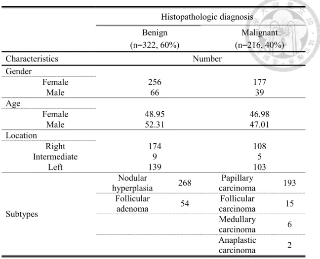
5.1.1 Materials ... 34
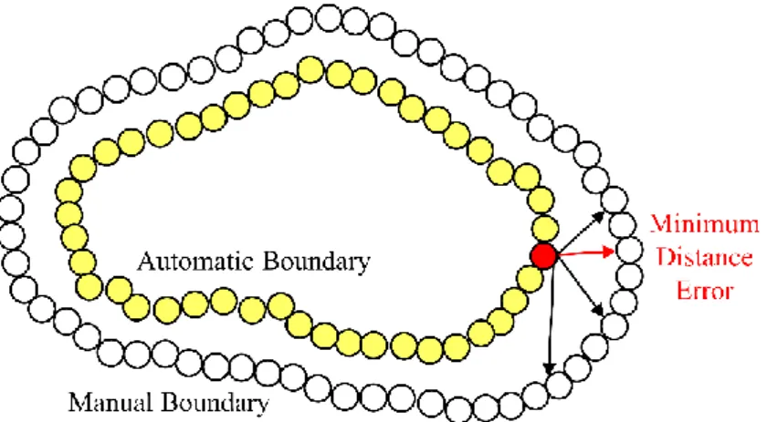
5.1.2 Performance analysis and evaluation ... 35
5.1.3 Results ... 39
5.2 Breast tumor detection in 3D ultrasound imaging ... 50
5.2.1 Materials ... 50
5.2.2 Performance Analysis and Evaluation ... 52
5.2.3 Results ... 53
Chapter 6 Discussions and conclusions ... 60
6.1 Boundary segmentation for ultrasonic thyroid nodules ... 60
6.1.1 Discussion ... 60
6.1.2 Conclusion ... 63
6.1.3 Future Research ... 63
6.2 Breast tumor detection in 3D ultrasound imaging ... 63
6.2.1 Discussion ... 63
6.2.2 Conclusion ... 66
6.2.3 Future Research ... 67
Reference ... 68
LIST OF FIGURES
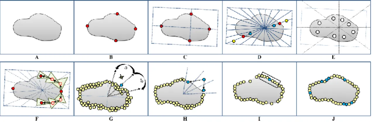
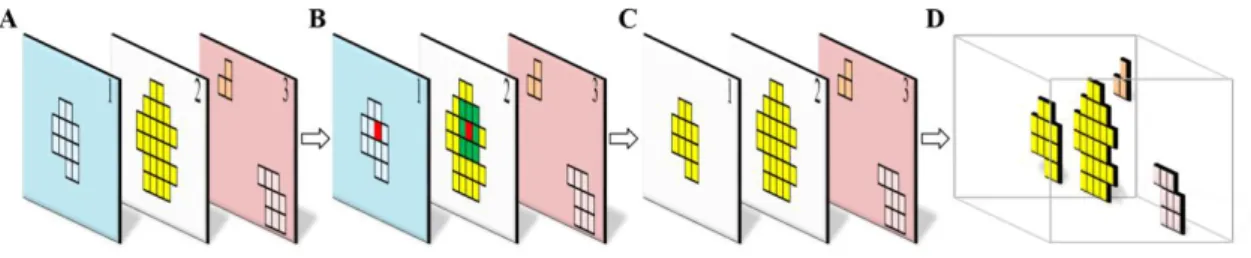
Fig. 3-1. The flow chart of our proposed method. ... 12 Fig. 3-2. Schematic diagram of semi-automatic segmentation of nodule boundary. (A) thyroid nodule. (B) manually input four extreme nodes on approximate location of the nodule. (C) the region of interest (ROI) was automatically generated based on the major axis and minor axis. (D) reference boundary points. (E) new cut points and new radial lines defined by the centers of the eight 45-degrees sectors in the ROI. (F) direction searching method. (G) outlier elimination method. (H) inner product method. (I) smoothing. (J) linking. ... 12 Fig. 3-3. The radial line was grown from the center of the ROI and then three cut points were searched on each radial line by Variance-Reduction statistic. ... 14 Fig. 4-1. The flow chart of our proposed CADe system. ... 19 Fig. 4-2. Steps of Image Preprocessing. (A) The original ABUS image. (B) The red rectangle showed the appropriate region for analysis excluding two lateral shadows. (C) The result of applying similar HE algorithm. ... 20 Fig. 4-3. Step-by-step visualization of 2D merge. (A) All pixels on image slice were cut into non-overlapping square cells. The upper one showed the schematic diagram of the square cells, and the lower one visualized each individual square cell with random color. (B) The appropriate analysis region set was a collection of the hypoechogenic square cells with average grayscale value lower than twenty-fifth percentile. (C) Adjacent appropriate analysis regions with similar grayscale values were merged together to form initial tumor candidates. ... 23 Fig. 4-4. 3D merge. (A) Tumor candidates from 2D phase were marked in different colors.
(B) Criterion of continuity: we searched a square cell belonging to one 2D
candidate and projected it onto corresponding position in neighboring slice.
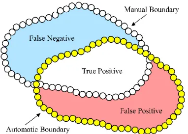
Then we checked if the projected square cell located in a 2D candidate on that slice or contacted with it in 8-connected manner. (C) 2D Candidates in slice 1 and slice 2 satisfied the criterion of continuity and thus merged together. The two 2D candidates on slice 3 were left untouched due to non-continuity. (D) The schematic view of image (C) in 3D space. The merged candidates (yellow) were referred as masses. ... 25 Fig. 4-5. Rim effect. While tumor grows, the tissues surrounding the tumor are compressed. Accordingly, tumor is generally accompanied with a thin rim of hyperechogenic tissues on ABUS images. ... 30 Fig. 5-1. The schematic diagram of the minimum distance error for every automatic boundary point. ... 36 Fig. 5-2. The schematic diagram of the corresponding area of FP, TP, and FN. ... 37 Fig. 5-3. Result of applying our proposed method on a benign case of thyroid nodule corresponding to the steps of Fig. 3-2. (A) original thyroid nodule on ultrasound image. (B) manually input four extreme nodes on approximate location of the nodule. (C) the region of interest (ROI) was automatically generated based on the major axis and minor axis. (D) reference boundary points. (E) new cut points and new radial lines defined by the centers of the eight 45-degrees sectors in the ROI. (F) direction searching method. (G) outlier elimination method. (H) inner product method. (I) smoothing. (J) linking. ... 39 Fig. 5-4. Result of applying our proposed method on a malignant case of thyroid nodule corresponding to the steps of Fig. 3-2. (A) original thyroid nodule on ultrasound image. (B) manually input four extreme nodes on approximate location of the nodule. (C) the region of interest (ROI) was automatically generated based on
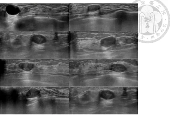
the major axis and minor axis. (D) reference boundary points. (E) new cut points and new radial lines defined by the centers of the eight 45-degrees sectors in the ROI. (F) direction searching method. (G) outlier elimination method. (H) inner product method. (I) smoothing. (J) linking. ... 40 Fig. 5-5. The comparison between the boundary generated by our proposed method and the gold-standard boundary by experienced radiologist. The first row were original images, the second row were the corresponding gold-standard boundaries, and the third row were the corresponding automatic boundaries, respectively. ... 41 Fig. 5-6. The comparison between the boundary generated by our proposed method and the gold-standard boundary by experienced radiologist on complicated cases.
The first row (Case A) was a nodule with weak boundary. The second row (Case B) was a nodule with blurring boundary. The third row (Case C) was a nodule with missing boundary. The fourth row (Case D) showed a nodule with intensity inhomogeneity. The fifth row (Case E) showed a case with cysts in nodule. . 43 Fig. 5-7. The screenshots of identical view of one benign nodule (Case A), one malignant nodule (Case B), and another malignant nodule with inhomogeneity (Case C), showing the results of comparison between our proposed method and other standardized methods. The first row were the original images, the second row were the gold-standard boundaries delineated by experienced radiologist, the third row were automatic boundaries by our proposed method, the fourth row were boundaries by Watershed Model, the fifth row were boundaries by Active Contour Model, the sixth row were boundaries by Distance Regularized Level Set Evolution, respectively. ... 44 Fig. 5-8. The detection results of applying our method on a benign (left column) and
malignant tumor (right column) corresponding to the steps, including 2D merge, 2D filter, 3D merge, and 3D filter. Each individual 2D candidate/3D mass was marked in random color on an image slice. (A) and (B) were original ABUS images. (C) and (D) were the results of 2D merge. (E) and (F) were the results of 2D filter. (G) and (H) were the results of 3D merge. (I) and (J) were the results of 3D filter, which showed excellent results of correct tumor detection without false positive. ... 54 Fig. 5-9. The examples of false positives in two conditions, false positive coexisting with true positive, and false positive existing alone in the normal pass. Each 2D candidate/3D mass was marked in random color on an image slice. (A) and (B) were original ABUS images. (C) and (D) were the results of 2D merge. (E) and (F) were the results of 2D filter. (G) and (H) were the results of 3D merge. (I) and (J) showed the results of 3D filter. In (I) and (J), red circle indicated the mass was true positive and uncirculated masses were false positives. ... 55
LIST OF TABLES
Table 5-1. Patient clinical data and nodule characteristics. ... 35
Table 5-2. The individual performance of our proposed method from training and testing datasets by using boundary error metrics and overlapping area metrics ... 47
Table 5-3. The individual performance of our proposed method from benign and malignant cases by using boundary error metrics and overlapping area metrics. ... 47
Table 5-4. The comparison of our proposed method with other methods by using the same dataset. ... 48
Table 5-5. Mann-Whitney U test p-values for method comparisons. ... 48
Table 5-6. Performance of different values of distance w. ... 49
Table 5-7. Performance of different values of angle θThreshold. ... 49
Table 5-8. Performance of different values of parameter a. ... 50
Table 5-9. Performance of different values of inner product b... 50
Table 5-10. Patient clinical data and tumor characteristics. ... 52
Table 5-11. The performance from four major parts of our proposed method. ... 57
Table 5-12. Mann-Whitney U test p-values and Student’s t-test p-values for different types of cases... 57
Table 5-13. Performance with different values of square size... 57
Table 5-14. Performance with different values of percentile of grayscale value. ... 58
Table 5-15. Performance with different values of Threshold for t-value t. ... 58
Table 5-16. Performance with different values of Threshold for f-value f. ... 58
Table 5-17. Performance variation with respect to parameters at 100% sensitivity. ... 58 Table 5-18. Comparison of performance in terms of sensitivity and corresponding FPs.
... 59
Chapter 1 Introduction
Ultrasound imaging is one of the most effective screening tools for the discovery of tumors. It possesses the advantages of non-invasiveness and irradiation-free, making it a suitable choice in regular screening. By interpreting the ultrasound images, doctors make decisions if the patients requires further examinations or interventions. However, the interpretation of ultrasound images are mostly subjective and highly depend on the experience and judgment of the operator, and the inter-observer variation often results in substantially different decisions. Due to these reasons, how to objectively and quantitatively describe a tumor in ultrasound imaging becomes a pressing issue facing the medical staffs.
To effectively quantify the sonographic features, an objective accurate tumor location and boundary have to be first determined. Therefore, computer-aided systems in our research are respectively proposed to automatically segment boundary of tumor and detect tumor location on ultrasound images.
1.1 Boundary segmentation for ultrasonic thyroid nodules
1.1.1 Background
Thyroid cancer has increased significantly over the past four decades in United States [1]. The advance in diagnostic tools allows the detection of small thyroid nodules [1]-[4].
Although early treatment is the key to the cure of cancer and further reduces the mortality rate [3], it may also lead to over-diagnosis with unnecessary biopsies and treatments [1]- [4]. Therefore, an appropriate screening tool with effective diagnosis ability has become an increasingly important issue [5]-[7].
Ultrasound imaging is one of the most effective non-invasive screening tools for the detection of thyroid nodules [6]-[14]. Beside conventional B-mode sonography,
elastography which reflects tissue stiffness plays a promising role in the characterization of thyroid nodules [17]. Based on impressions of observing the ultrasound images, clinicians make suggestions for patients to be subject to periodic follow-up or further cytological tests [8]. However, the acquisition and observation of ultrasound images are mostly subjective and highly depend on the experience and judgment of the operator, and the inter-observer variation often results in significantly different decisions [6], [11]-[13].
According to aforementioned reasons, objective quantification of the sonographic thyroid nodule features has become a pressing issue facing the medical staffs [6]. To effectively quantify the sonographic features, an objective accurate nodule boundary has to be first determined. Therefore, computer-aided system was proposed to automatically detect and identify the boundary of thyroid nodules on ultrasound images [9]-[14].
1.1.2 Objective
For computer-aided systems, speckle is one of the most challenging problems [9]- [14], [15], [16]. To reduce the impact of speckle, previous publications used image preprocessing methods or altered the detailed information provided during the execution steps [9]-[11], [14]. However, speckle also carries information about tissue characteristics and may be exploited in several applications. Approaches in attempt to reduce speckle may result in the loss of such information within original ultrasound images, and may even affect the capturing of nodule features and the correctness of the computer-aided system operation.
To the best of our knowledge, this is the first work to apply Variance-Reduction (V- R) statistics-based approach to detect nodule boundaries on thyroid ultrasonography. In this study, we propose a novel and semi-automatic method without image preprocessing.
1.2 Breast tumor detection in 3D ultrasound imaging 1.2.1 Background
Breast cancer has the highest incidence and causes the second leading mortality of cancer among women in 2017 in the United States [18]. Since early treatment is the key to the cure of breast cancer, effective diagnosis system and the adjunctive detection system have become an important issue to further reduce the mortality rate [19].
Mammography [20] and breast ultrasound [21] are two of the most commonly used screening tools for the diagnosis and detection of breast tumor. Each of them has its own advantage and disadvantage in clinical examination [22]. Mammography is adopted as a major screening tool for its high sensitivity in detecting micro-calcification and can be used to further detect early changes in abnormal tissues, but it also suffers from high false positive rate especially in women with dense breast tissue [23]-[26]. Breast ultrasound is the most important alternative to mammography [23]-[25], with the advantages of radiation-free and less pain, but ultrasound imaging highly depends on the medical staff’s experience and judgment, resulting in inter-observer variations that often lead to significantly different clinical decisions, and the results are poorly reproducible [26].
Based on these problems, automated breast volume scanner (ABVS) as an innovative high-end ultrasound scanner has been developed by combining the advantages of mammography and breast ultrasound to automatically scan the entire breast [9]-[11].
Additionally, ABVS allows the scan results to have less operator dependency and higher reproducibility, and provides coronal images to further assist the planning of surgical intervention [26], [27]. However, the reviewing process to discover suspicious abnormalities from hundreds of image slices produced by ABVS is often time-consuming [29], [30]. Besides, tumor which is tiny or isoechogenic to the surrounding normal tissue
may be missed by reviewer [30]. Therefore, computer-aided detection (CADe) system has been proposed to accelerate the reviewing process and to reduce the missing errors [33]-[39]. As defined by the U.S. FDA, “CADe devices are computerized systems that incorporate pattern recognition and data analysis capabilities and are intended to identify, mark, highlight, or in any other manner direct attention to portions of an image, or aspects of radiology device data, that may reveal abnormalities during interpretation of patient radiology images or patient radiology device data by the intended user” [40]. CADe system is needed to solve a practical clinical problem of ABVS where thousands of images were acquired by automatically scanning the patient breasts and will be time- consuming and tiresome for physicians to review the slice one by one to discover any suspicious lesions.
1.2.2 Objective
The aim of this study is to develop an intuitive, simple, efficient CADe solution to quickly screen all the images generated by the automated three-dimensional breast ultrasound (ABUS), in particular Siemens ACUSON2000 ABVS in this study, to highlight all possible lesions for further review and diagnosis by physicians.
Chapter 2 Literature Review
In this chapter, the discussion of our research is separated into two topics: boundary segmentation for ultrasonic thyroid nodules and breast tumor detection in 3D ultrasound imaging. For each topic, we will review related works and summarize the advantages and disadvantages. Then, we will introduce some of the methods related to our proposed methods.
2.1 Boundary segmentation for ultrasonic thyroid nodules
Various methods have been employed for computer-aided systems to automatically detect and identify the boundary of thyroid nodules on ultrasound images.
Tsantis et al. [9] proposed a hybrid multi-scale model which integrated the wavelet edge detection procedure and the Hough transform to extract the final contour of thyroid nodules in ultrasound images. This method was advantageous by combining the ability of wavelet transform to detect sharp variation and the efficiency of Hough transform to discriminate target from noisy background. Nevertheless, it also had several shortcomings that the delineation outcome was highly affected by human error, and the step of Hough transform was time-consuming. Besides, it required prior knowledge about the shape of nodule to be detected, which limited the value in practical use. Iakovidis et al.[10]
presented a segmentation framework applied on thyroid ultrasonography by incorporating a level set approach named Variable Background Active Contour model and a parameter tuning mechanism based on Genetic Algorithm to search for optimal parameters automatically. This GA-VBAC framework was relatively unaffected by intensity inhomogeneity in the thyroid ultrasound images. However, this method required huge amount of time in its training phase, which posed a major limitation. Maroulis et al.[11]
developed an algorithm of Variable Background Active Contour model based on the
Active Contour Without Edges model for the delineation of thyroid nodules in ultrasound images. This algorithm had the advantages of noise robustness, multiple nodules delineation capability, and the ability to cope with intensity inhomogeneity. One of the drawbacks of their proposed algorithm was that it could not delineate non-hypoechoic thyroid nodules. Savelonas et al. [12] presented a joint echogenicity–texture model based on a modified Mumford–Shah function that incorporated regional image intensity and statistical texture information. Their approach were capable of segmenting hypoechoic, isoechoic, and hyperechoic nodules. It required no prior assumption about the shape of nodule to be detected, and was noise-tolerant. Nevertheless, it also had some limitation that it might get confused by anatomical structures within nodules such as blood vessels.
Koundal et al.[14] proposed an automated delineation method that integrated spatial information with the Neutrosophic L-Means clustering and level-sets method for the segmentation of thyroid nodules in ultrasound images. This method first segmented possible target via Spatial Neutrosophic L-Means clustering, then applied Distance Regularizer Level Set Evolution method to delineate the nodule contour. It had benefits of noise robustness and multiple nodules delineation capability, and could handle intensity inhomogeneity as well. However, it had weakness in its ability to detect isoechoic thyroid nodules. Ma et al. [31] employed a deep convolutional neural network for thyroid nodule segmentation based on 2D ultrasound images. The convolutional neural network was fed with image patches from thyroid nodules and normal thyroid as input, then output the segmentation probability. This method could delineate thyroid nodules accurately and was capable of multiple nodules delineation. It was also noise- tolerant. Despite of these, this deep-learning based method showed unsatisfying performance while dealing with heterogeneous nodules or complicated background.
Chang et al. [32] developed a method to retrieve thyroid nodule contour on the basis of a
manual input contour. The manual input contour was then processed with Active Contour Method into a smooth thyroid nodule contour, and the sonographic features of the region enclosed by the contour were calculated.
In recent years, deep learning has gradually been discussed and valued in various field of applications. Among them convolutional neural network (CNN), such as Ma et al. [31]
used in their work, has gained the most attention. However, unlike traditional knowledge- based methods, the “black-box” nature of these CNN-based system may lead to severe consequences and arouses incremental concerns recently. CNN requires huge amount of ground truth data for training, and we even do not know what it learns, how it learns, and where it errs.
The region of interest (ROI) delineation usually plays an important role in ultrasound image analysis. With ROI being delineated, the computation cost of ultrasound image analysis is greatly reduced, and the accuracy is improved. However, the delineation of ROI for ultrasound images is not always readily available in clinical settings. It adds an extra step beyond the standard operations of ultrasound imaging, and the ROI delineation step itself is error-prone if not performed by experienced operator. To take advantage of ROI delineation and simultaneously avoid its drawback, it is essential to incorporate the step of ROI delineation with the standard operation procedures of ultrasound examinations.
2.2 Breast tumor detection in 3D ultrasound imaging
Computer-aided detection system has been proposed to accelerate the reviewing process and to reduce the missing errors. Recently, the issue has received special attention and discussion in the 3D ultrasound images.
Ikedo et al. [33] proposed a fully automatic scheme based on the edge information
detected by Canny edge detector and further classified edges as near-vertical edges or near-horizontal edges by a morphological method. Initial tumor candidate regions were then generated by watershed algorithm and density information among the region with near-vertical edges. This method achieved sensitivity of 80.6% to detect breast tumor, but has difficulty in detecting flat-shaped tumors due to their short vertical dimensions.
Besides, it frequently misinterpreted fat and rib regions. Chang et al. [34] used the gray- level slicing method to segment images into numerous regions, and then seven quantitative features were extracted to further determine each region whether a part of tumor or not. Their proposed system achieved decent sensitivity of 92.3%, but had a long processing time. Besides, the case number in this study was small, which hampered the reliability of their conclusion. Moon et al. [35] developed a CADe system based on algorithm of Hessian analysis with multi-scale blob detection. Then three categories of quantitative features were extracted to estimate the tumor likelihood with a logistic regression model. Their proposed system could detect every tumor and achieved the sensitivity of 100%, but accompanied with a lot of erroneous detections. Besides, their study did not involve early-stage breast cancers, so the ability of detecting small malignant tumors was unknown. Tan et al. [36] presented a two-stage CADe system.
After landmarks such as nipple and chest wall were provided, tumor candidates were generated by using voxel features including coronal spiculation patterns, blobness, and contrast. The likelihood of malignancy was evaluated with an ensemble of five neural networks. A major shortcoming of their proposed system was that the maximal achievable sensitivity was suboptimal. Moon et al. [37] proposed a CADe system based on quantitative tissue clustering algorithm. The fuzzy c-means clustering was used to generate tumor candidates among the regions segmented by fast 3D mean shift method.
Seven quantitative features were used to estimate the likelihood of the candidates being
tumors. A limitation of their study was the high false positive rate, which could be a problem for clinical applications of CADe systems. Lo et al. [38] proposed a CADe system based on topographic watershed transform gathering similar tissues around local minima into homogeneous regions. The likelihood of region being tumor was determined with quantitative features of morphology, echogenicity, and texture. The proposed CADe system achieved the sensitivity of 100% with tolerable false positive rates. Besides, the processing time was satisfactory. There were some limitations in their study though. Their system might not perform well for all kinds of breast carcinomas. Furthermore, the data used in their study all came from a single medical center and might hinder the generalization of their system.
Utilizing deep learning, Chiang et al. [39] proposed a method based on 3D convolutional neural networks and prioritized candidate aggregation. Their proposed system first implemented a sliding window detector to extract volume of interest, which were then determined their tumor probability by 3D convolutional neural networks. Their proposed system was advantageous for its fast processing time. However, a major drawback of their proposed system was that it did not perform well at high sensitivities and produced a lot of false positives.
Decision tree learning is one of the predictive modelling approaches used in statistics, data mining, and machine learning. Among them, classification and regression tree (CART) [41] is one of the most well-known models. CART is constructed through a sequential binary classification, and its goal is to make the child nodes with a higher homogeneity. The first stage is to build a complete classification tree. At this stage, subjects are binary-classified over and over until classification is no longer possible. The method will search for the best feature and cut point in the parent node, and then use this feature and cut point to divide the parent node into two child nodes. If the number of
samples of the child node is too small or the child node has only one category left, then the classification will stop; otherwise, the classification will continue. A complete classification tree is established through the complete classification of training samples, but it usually leads to the problem of over-fitting. Therefore in the second stage, some branches of the complete classification tree need to be pruned to avoid over-fitting.
We construct our detection algorithm inspired by CART, to implement the free-of- parameters advantage thus ideal for our application to analyze huge amount of data contained within 3D ultrasound images.
Chapter 3 Variance-reduction methods for boundary segmentation
In this study, we developed a novel and semi-automatic system to detect the boundary from thyroid nodule on ultrasound images. The architecture of our proposed method in this chapter was shown as flow chart and schematic diagram in Fig. 3-1 and Fig. 3-2, respectively. Firstly, region of interest (ROI) was automatically generated according to the initial inputs of the nodule’s major and minor axes. Subsequently, the boundary candidate points were extracted using the V-R statistics. Three filtering methods including the direction searching method, the outlier elimination method, and the inner product method were used in sequence to further filter out the outliers among the remaining boundary candidate points of the previous step. The remaining boundary candidate points were then smoothened and linked together to form the final boundary.
Fig. 3-1. The flow chart of our proposed method.
Fig. 3-2. Schematic diagram of semi-automatic segmentation of nodule boundary. (A) thyroid nodule. (B) manually input four extreme nodes on approximate location of the nodule. (C) the region of interest (ROI) was automatically generated based on the major
axis and minor axis. (D) reference boundary points. (E) new cut points and new radial lines defined by the centers of the eight 45-degrees sectors in the ROI. (F) direction searching method. (G) outlier elimination method. (H) inner product method. (I) smoothing. (J) linking.
3.1 Boundary Candidate Extraction
The nodule boundary on the ultrasound image was generally characterized by significant difference in grayscale values between the inside and outside of the nodule boundary. Therefore, we proposed a method that automatically detects the thyroid nodule boundary with segmentation and identification methods by combining the radial gradient algorithm and the V-R statistics.
3.1.1 ROI automatic generation
Before the proposed method was implemented, the ROI was automatically generated based on the approximate major axis and minor axis of the nodule manually input by medical staff, as shown in Fig. 3-2 (A) to (C).
3.1.2 Reference boundary points
The radial lines were then grown from the center of the ROI and three original cut points on each radial line were searched by the V-R statistics so that each cut point resulted in minimum sum of two group total sum of square, as in (3-1), Fig. 3-2 (D) and Fig. 3-3.
1 2 2
1 2
1 1
min
a N
i i
a i i a
x μ x μ
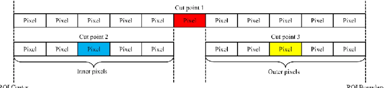
(3-1) In (3-1) and corresponding Fig. 3-3, a radial line has N pixel points and their grayscale values are represented as a set {x1, x2, …, xa, …, xN-1, xN} where xi is the grayscale value of the pixel point i in the order from the ROI center to the ROI boundary, and μ1 and μ2are the averages of grayscale values of the inner pixels and outer pixels which are separated by pixel point a, respectively. After searching pixel point a throughout N pixel points, the first cut point is defined as the one resulting in minimal sum of two total sum of squares and further marked with red. Moreover, two additional cut points are defined by repeating the above process from inner and outer segments of the radial line separated by the first cut point. The two newly generated cut points are then marked with blue and yellow, respectively, as shown in Fig. 3-2 (D) and Fig. 3-3. Three original cut points from all radial lines are regarded as reference boundary points.
Fig. 3-3. The radial line was grown from the center of the ROI and then three cut points were searched on each radial line by Variance-Reduction statistic.
3.1.3 Boundary candidate points
In order to prevent the influence from the variation of the nodule’s inner tissues, we further searched more useful cut points based on (3-1) and the reference boundary points.
Firstly, new radial lines were defined by the new centers of the reference boundary points within eight 45- degrees sectors in the ROI, as shown in Fig. 3-2 (E). Secondly, three cut points were generated by applying (3-1) on each new radial lines and were then regarded as boundary candidate points.
3.2 Filtering
With the plenty boundary candidate points extracted by the V-R statistics, we needed to determine which candidate points were more likely to be located on the nodule boundary. To further obtain suitable boundary candidate points, we developed three filtering methods including the direction searching method, the outlier elimination method, and the inner product method.
The filtering methods were executed based on the information of the four nodes, which provided approximate locations of the nodule boundary points. The nodule boundary ought to go through these four nodes, so our filtering method worked in a manner that boundary candidate points should be on the path going through these four nodes.
3.2.1 Direction searching method
The direction searching method started from one of the four nodes and defined the feasible region according to the path direction from one node served as initial starting point toward its two neighboring nodes, respectively. The path was further divided into many parts to increase the number of searching steps in order to ensure accuracy. The searching condition was set as that if a boundary candidate point was located in the feasible region and satisfied the criterion of the distance from the starting point, then it was preserved, otherwise it would be filtered as in (3-2).
dij w or θnij θThreshold (3-2) In (3-2), dij represents the distance between starting point i and the boundary candidate point j, w is a parameter tuning the threshold. θnij represents the angle formed by neighboring node n, starting point i and boundary candidate point j. θThreshold represents the feasible region.
The process was separately performed on both sides of the initial starting point, iteratively replacing the starting point by the center of the points satisfying the condition in previous step, and gradually decreasing the feasible region in each iteration to ensure convergence onto the neighboring nodes. The iteration stopped at the arrival of the two neighboring nodes, and then the above process restarted with another node as a new initial starting point. Finally, the whole process ceased after all four nodes completed the searching process, as shown in Fig. 3-2 (F).
3.2.2 Outlier elimination method
Since an appropriate nodule boundary should not have candidate points extremely outlying from other points, the outlier elimination method and the inner product method were used after the direction searching step to eliminate these outlier points.
The outlier elimination method was implemented to filter out the boundary candidate points which were relatively distant from other boundary candidate points in a sector area, as shown in (3-3) and Fig. 3-2 (G).
ic K K
d μ aσ (3-3) In (3-3), there are k boundary candidate points in the sector area K, and the distance between the ith boundary candidate point and the center of ROI are represented as the set of {d1c, d2c, …, dic, …, d(k-1)c, dkc }. μK and σK are the mean and standard deviation of all distance values in the sector area K, respectively, and a is a parameter tuning the threshold.
3.2.3 Inner product method
The inner product method filtered out the boundary candidate points resulting in a sharp angle between two neighboring boundary candidate points, as shown in (3-4) and Fig. 3-2 (H).
Vi i(1) Vi i(1)
b (3-4)In (3-4), we sort all boundary candidate points in order, where 𝑉⃑ 𝑖(𝑖−1) and 𝑉⃑ 𝑖(𝑖+1) are vectors from boundary candidate point i to its two neighboring boundary candidate points (i-1) and (i+1), respectively, and b is a parameter tuning the threshold.
3.3 Smoothing and Linking
After these three filtering steps, the remaining boundary candidate points were smoothened (Fig. 3-2 (I) and (3-5)), and extra points were filled in to link the distant neighboring boundary candidate points to form the final boundary (Fig. 3-2 (J)).
Smoothing process applied a pulling effect on each remaining boundary candidate point from its surrounding neighborhoods, in order to smoothen the extreme convexity or concavity of the remaining boundary candidate points, as in Fig. 3-2 (I) and (3-5).
( , ) ( , )
2 1 2 1
i s i s
w w
w i s w i s
i i
X Y
X Y s s
(3-5) Equation (3-5) shows the new coordinate (Xi’, Yi’) of the boundary candidate point i which is smoothened by taking the average of coordinates from the (i-s)th candidate point to the (i+s)th candidate point.
The linking process took place when a boundary candidate point i and its neighbor point i+1 were not adjacent in 8-connected manner. Then the extra points were added to the line connecting point i and point i+1 to fill the gap. The linking process repeated until there was no gap in the boundary. The extra points filled in were shown with blue color in Fig. 3-2 (J).
Chapter 4 Two-phase merge-filter methods for 3D tumor detection
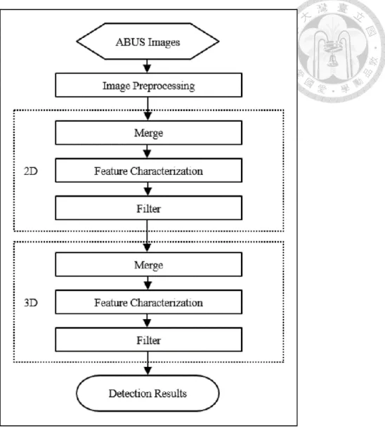
We developed an intuitive, simple, efficient, and automatic CADe system to detect breast tumor on ABUS images. The detection method proposed in this chapter was shown in Fig. 4-1 and described as follows.
The detection method was performed in a two-phase manner. First, in two- dimensional (2D) phase, after image preprocessing, square cells with hypoechogenicity and homogeneous texture were extracted and merged into initial tumor candidates [50].
Intensity-related features were then generated to characterize the 2D candidates to subsequently distinguish tumors from non-tumors. A classifier was then constructed to stage-wise classify 2D candidates and to filter out non-tumor ones efficiently. Secondly, in three-dimensional (3D) phase, remaining 2D candidates were merged longitudinally into 3D masses, and the merged 3D masses were then characterized by four types of features. Finally, the classifier was used again based on 3D features to further filter out non-tumor masses to obtain the final detected masses.
Fig. 4-1. The flow chart of our proposed CADe system.
4.1 Image Preprocessing
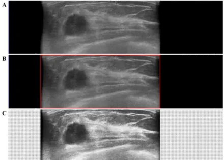
The ABUS image pass consists a series of 318 slices with plenty pixel points providing lots of image data information. Because of this, the analysis of the ABUS images is usually a time-consuming reviewing process [29], [30]. Therefore, according to the subtle variation between the image slices [38], we extracted one image slice from every five slices for better efficiency. Furthermore, to acquire an appropriate image region for subsequent analysis, we excluded two lateral shadow regions in each image which were caused by the gap between the transducer and the breast skin during scanning. The
result of the appropriate region of interest for analysis was shown in Fig. 4-2 (B).
Ultrasound images generally contain plenty of speckle and low contrast due to the complex imaging environment and imaging principle. Accordingly, the quality of the ultrasound image may be diminished, resulting in ineffective diagnosis or interpretation.
Besides, ultrasound images may appear globally dark or bright between different image slices, and this leads to an unfavorable phenomenon in dealing with an image pass.
Histogram equalization (HE) [50], [51] is a famous methods for image processing to enhance contrast [52] and uniform the probability distribution of the grayscale values without destructing the important features. However, HE may enhance meaningless detail and hide important but small high-contrast features [53]. To avoid these effect, we applied a modified HE algorithm contributed by Richard Kirk [53] combining a transformation function by using the square root of the histogram values. After preprocessing, images in each pass had uniform grayscale distribution and showed more detail in the suspicious regions. The result was shown in Fig. 4-2 (C).
Fig. 4-2. Steps of Image Preprocessing. (A) The original ABUS image. (B) The red rectangle showed the appropriate region for analysis excluding two lateral shadows. (C)
4.2 2D merge
In this step, we intended to extract candidates for the region that likely to be tumor.
According to clinical experience, tissues within the tumor region usually have similar echotextures [37]. The procedure was taken in three steps, not only extracted the initial candidates, but also reduced the processing time for the subsequent steps.
Firstly, all pixel points on an image slice were cut into non-overlapping square cells, as shown in Fig. 4-3 (A). Secondly, owing to the hypoechogenicity of breast tumors [37], we collected the square cells with average grayscale value lower than twenty-fifth percentile among all grayscale values within an image slice. The collection of these hypoechogenic square cells were regarded as a set of appropriate analysis regions, as shown in Fig. 4-3 (B).
Thirdly, if two adjacent appropriate analysis regions were similar in grayscale values, they were merged together. Modified t-statistic and F-statistic were adopted to judge similarity in grayscale values due to clinical observation that tumor region usually has similar echotextures [37]. Two adjacent appropriate analysis regions satisfying the following two criteria were merged together: similarity in average grayscale values judged by modified t-statistic and similarity in standard deviations of grayscale values judged by F-statistic[57]. Furthermore, the denominator used in modified t-statistic was changed to the square root of overall average variance from all appropriate analysis regions to avoid the effect of outliers on an image slice. Modified t-statistic and F-statistic were formulated as (4-1) and (4-2), respectively.
2
( ) 1
Ni m m
jk j k
i
T μ μ σ t
N
(4-1)2
2 2
2
2
2 2
2 j
j k
k
k
j k
j
σ f if σ σ
F σ
σ f if σ σ
σ
, ,
(4-2)
If an image slice i contains Ni appropriate analysis region, and region j contains texture information about mean grayscale value μj and standard deviation value σj. Tjk and F represent the modified t-value and F-value between two adjacent regions j and k,
respectively, where j < k. t and f are parameters tuning the threshold for Tjk and F, respectively.
The merging procedure was iteratively performed until there were no adjacent region composing statistically similar tissue texture. The products of merging procedure were referred as initial tumor candidates, as shown in Fig. 4-3 (C). The scheme of whole mergence procedure was demonstrated in Fig. 4-3.
Fig. 4-3. Step-by-step visualization of 2D merge. (A) All pixels on image slice were cut into non-overlapping square cells. The upper one showed the schematic diagram of the square cells, and the lower one visualized each individual square cell with random color.
(B) The appropriate analysis region set was a collection of the hypoechogenic square cells with average grayscale value lower than twenty-fifth percentile. (C) Adjacent appropriate analysis regions with similar grayscale values were merged together to form initial tumor candidates.
4.3 2D Features Characterization
After 2D merge, these regions were regarded as initial tumor candidates. However, too many candidates among non-tumor areas may cause prolonged processing time, poor performance, and frequent false positives (FPs). To further distinguish tumor from non- tumor candidates, we extracted intensity-related features in 2D phase to characterize candidates in ABUS images[54]-[56].
The intensity of candidate within tumor region is generally darker than that of the surrounding tissues. Based on this characteristics, two intensity-related features were generated to distinguish tumor and non-tumor candidates, namely intensity mean value (I(c)mean, defined in (4-3)) and the percentile of I(c)mean within the image slice (Percentile_I(c)mean).
1
(c)mean p
c p c
I I
n
(4-3)Candidate c has a set of pixel points {p}, and the amount of pixel points in c is nc. Ip
indicates the grayscale value of pixel point p within candidate c.
4.4 3D merge
The 3D phase of our proposed detection method began with an algorithm of 3D merge.
2D candidates in neighboring transverse image slices which met the criterion of continuity were then merged longitudinally by volume growth characteristics. Finally, the merged 3D objects were referred as masses.
The criterion of continuity were based on the fact that tumors generally distribute in a spatially continuous manner. First, we searched a square cell belonging to one 2D candidate and projected it onto corresponding position in neighboring slice. Then we checked if the projected square cell located in a 2D candidate on that slice or contacted
with it in 8-connected manner. If so, then the two 2D candidate were merged together because of high likelihood belonging to the same tumor. The procedure iteratively repeated until there were no 2D candidates meeting the criterion of continuity. The schematic diagram was shown in Fig. 4-4.
Fig. 4-4. 3D merge. (A) Tumor candidates from 2D phase were marked in different colors.
(B) Criterion of continuity: we searched a square cell belonging to one 2D candidate and projected it onto corresponding position in neighboring slice. Then we checked if the projected square cell located in a 2D candidate on that slice or contacted with it in 8- connected manner. (C) 2D Candidates in slice 1 and slice 2 satisfied the criterion of continuity and thus merged together. The two 2D candidates on slice 3 were left untouched due to non-continuity. (D) The schematic view of image (C) in 3D space. The merged candidates (yellow) were referred as masses.
4.5 3D Features Characterization
To further improve the performance after 3D merge, we extracted four types of features to characterize 3D masses in ABUS images for further classification between tumor and non-tumor [54]-[56]. The features extracted are solely for lesion detection and are different from those features specified in BIRADS for breast cancer diagnosis.
4.5.1 Morphology
Morphology features were mainly quantified from the relevant information of the 3D mass boundary and provided the most useful and direct information for tumor detection.
We implemented eight morphological features in three major categories: size-related features, shape-related feature, and aggregation-related feature.
Four size-related features, the size of mass (Size), Length, Width, and Height, were implemented to exclude speckles and shadows in ABUS images. The speckles appearing in ABUS images are small, whereas the shadows shown in the bottom, near-nipple region, and two lateral sides usually occupy a large area. Consequently, Size could be used to filter masses with extremely small or extremely large size. The Length, Width, and Height were the dimensions of the minimal bounding cube containing the mass. These three features were auxiliary to help distinguish speckles and shadows in ABUS images.
Three shape-related features including the Length-to-Width ratio (RatioL-W), Length- to-Height ratio (RatioL-H), and Width-to-Height ratio (RatioW-H) were introduced to filter outliers such as fat, ribs, and shadows in ABUS images. Fat tissues generally have flat and thin shape in horizontal plane, while the ribs are as dark as tumor in ABUS images but have RatioW-H around 1. Shadows described above generally have narrow Width and span across several image slices leading to a large RatioL-W. According to these properties, the ratios were introduced to filter the fat-like masses (large RatioL-H or large RatioW-H), rib-like ones (RatioW-H around 1), and shadow-like ones (large RatioL-W). The definitions of three ratios were shown in (4-4), (4-5), and (4-6), respectively.
L W
Length Ratio
Width
(4-4)
L H
Length Ratio
Height
(4-5)
W H
Width Ratio
Height
(4-6)
The aggregation-related feature was the ratio of size-to-bounding cube (RatioS-B). This feature was defined to describe the aggregation of the mass. A mass with higher degree of aggregation was more likely to be a tumor. The RatioS-B was defined as (4-7).
S B Size
Ratio
Length Width Height
(4-7)
4.5.2 Texture
We generated five texture-related features in the 3D phase. The main three of the five features, I(m)mean, I(m)stdev, and the coefficient of variation (CV(m)), were used to distinguish tumor from non-tumor masses. Their definitions were shown in (4-8), (4-9), and (4-10), respectively.
( )mean 1 p
m p m
I m I
n
(4-8)
2( )stdev 1 p ( )mean
m p m
I m I I m
n
(4-9)( ) ( )
( )
stdev mean
CV m I m
I m (4-10) Mass m has a set of voxel points {p}, and the amount of voxel points in m is nm. Ip
indicates the grayscale value of voxel point p within mass m.
Furthermore, to get rid of the influence from the different distribution of the intensity between slices and to consider the relative echogenic characteristics within single image slice, we implemented another two texture features, the rank ratio of intensity mean value (IR(m)mean) and the rank ratio of intensity standard deviation (IR(m)stdev) among all masses M in a pass, as an auxiliary consideration. The definitions of these two texture features were shown in (4-11) and (4-12), respectively. |M| represents the number of all masses in a pass.
( )
( )mean m M mean Rank I m
IR m M
(4-11)
( )
( )stdev m M stdev
Rank I m
IR m M
(4-12)
4.5.3 Location
Four location features were generated based on the anatomy of the breast and the interpretation of ABUS images. The breast tissues generally distribute obliquely from the superior-lateral to inferior-medial side. Consequently, the location of the 3D mass in foot- to-head direction (LocationF-H) was implemented as one of the features.
In ABUS images, ribs sometimes look similar to breast tumors. To exclude the ribs, we introduced a feature in addition to aforementioned morphology features, Depth, according to the fact that the distance between skin and rib is greater than that between skin and breast tumor. In other words, the masses in the rib region usually have a large Depth. Furthermore, the rank ratio of Depth (DR) with respect to all masses in a pass was
also considered as location feature to further filter out the outliers.
Besides, nipple often results in shadows on ABUS images. To exclude these shadows, we introduced a feature, normalized distance between mass and nipple marker (DistanceM-N), to improve the performance of filtering. This feature also helped us ruling out lateral shadows extremely far from the nipple. To normalize the effect of breast size between people, DistanceM-N was derived by the ratio of measured mass-to-nipple distance relative to the width of breast. DistanceM-N was based on operator-input nipple marker, which is an essential step required by ABVS Workplace system to finalize the examination [58]. Due to the existence and correctness of the nipple marker, we used this as a-priori knowledge to generate the feature.
4.5.4 Rim Effect
We considered the tissue characteristic on ABUS images regarding the relationship between tumor and surrounding breast tissue. Breast tumor generally appears darker than surrounding tissue and grows from the mammary gland and is encircled by it. While tumor grows, tissue surrounding the tumor is compressed. Accordingly, tumor is generally accompanied with a thin rim of hyperechogenic tissue on the ABUS images and has obvious intensity difference from the tumor interior, as shown in Fig. 4-5. A total six features were constructed to describe this fact, including the maximum upper variance (VarU, defined in (4-13)), the maximum lower variance (VarL, defined in (4-14)), the sum of these two variances (VarUL, defined in (4-15)), and the respective rank ratio of these three features within a pass.
max min
min
2
, ,
min
, ,( 1) ,( 1) ,
max 1 ,
1 ...
c
i
a a b b
y x
u j x x i x y
c y y
U u J u J u J u J
Var I x y μ
y y
Var Var Var Var Var
(4-13)
max max
min
2
, ,
max
, ,( 1) ,( 1) ,
max 1 ,
1 ...
i c
a a b b
y x
l j x x i x y
c y y
L l J l J l J l J
Var I x y μ
y y
Var Var Var Var Var
(4-14)UL U L
Var Var Var (4-15) In (4-13), Varu,j is the maximum variances of the vertical line segments between the horizontal axis of this area’s center and the uppermost of ROI, calculating over a range from the minimal x-coordinate to the maximal x-coordinate of the partial area of the mass on image slice j. VarU sums Varu,j over the range from image slice Ja to image slice Jb in which the corresponding mass exists. In (4-14), VarL is difined similarily regarding the opposite half of ROI.
Fig. 4-5. Rim effect. While tumor grows, the tissues surrounding the tumor are compressed. Accordingly, tumor is generally accompanied with a thin rim of hyperechogenic tissues on ABUS images.
4.6 2D filter/ 3D filter
To further reduce the FPs from 2D candidates and 3D masses, a classifier was constructed by using an intuitive and efficient method applying stage-wise classification onto 2D features and 3D features.
The procedure began with all 2D candidates/3D masses involved to distinguish tumors from non-tumors through the classifier. The optimal cut-point for each feature resulting in best reduction ability was first automatically determined from all 2D candidates/3D masses. For 2D filter, the best reduction ability was defined by least false positives at 100% sensitivity. For 3D filter, the best reduction ability was defined by two criteria, the least false positives at 100% sensitivity, and the closest-to-(0, 1) criterion as in (4-16)[59]. If no cut-point with best reduction ability could be determined, then the
with best performance was automatically determined by the least false positives among all optimal cut-points. Then the feature with best performance was used to classify 2D candidates/3D masses into tumors and non-tumors. To reduce the processing time, 2D candidates/3D masses which were classified as non-tumors were discarded directly at each iteration, and this feature was no longer used thereafter. The next iteration involved the remaining 2D candidates/3D masses from previous iteration, automatically determined the feature with best performance among unused features, and classified remaining 2D candidates/3D masses. The iteration of classification stopped when all features have been used.
The determination of optimal cut-point, the choice of feature with best performance, and classification were all fully automatic, without parameters or human intervention.
Algorithm for classifier
A. Initialization:
Step 1. Collected all feature values from all 2D candidates/3D masses as an input dataset S
Step 2. Statistical normalization of S B. Iteration t:
Step 1. For each feature i, optimal cut-points Ci was determined by searching throughout all 2D candidate/3D mass j satisfying the best reduction ability at 100%
sensitivity:
i. In 2D filter: Xi minj
FPjii. In 3D filter:
2 2
, (1 j ) (1 j )
i j
j j j j
TP TN
Y TP FN TN FP
, Zi j, FPj (4-16)