基於子空間映射與多臂吃角子老虎機技術之實數最佳化

(1)

國立臺灣大學電機資訊學院電機工程學系碩士論文

Department of Electrical Engineering

College of Electrical Engineering and Computer Science

National Taiwan University Master Thesis

基於子空間映射與多臂吃角子老虎機技術之實數最佳化

Real-valued Optimization by Subspace Projection and Multi-armed Bandit Techniques

彭俊人 Chun-Jen Peng

指導教授：于天立博士 Advisor: Tian-Li Yu, Ph.D.

中華民國 106 年 7 月 July, 2017

(2)

(3)

誌謝

首先，我要感謝于天立教授從專題到碩士班一路的指導。于教授是我心中的學者典範，不只是其聰明才智的展現，更多的是在做學問上的態度。于教授不只研究嚴謹，更用其自身的作為讓我們理解到，不但要盡力把每件事情做好，作為學者更是要要對自己說的每一句話負責任。同時也很感謝于老師在研究之外對我們學生的關心，並很樂意花額外的時間與我們分享人生的經驗。在我研究遇到挫折時，除了能在極短的時間裡具體地指出我的盲點，更是能給我非常多有用的建議與哲理，充分地給予我思想與實質上的寶貴意見。非常慶幸一路上有于教授的指導，讓我能完成碩士論文。

其次，我要感謝蔡秉璇同學與于天立教授對於多臂吃角子老虎機技術的理論推導與想法貢獻。很感謝秉璇不厭其煩的教我其中的理論推導，並且在嘗試投稿時分擔了大部分的工作。並且在我進度落後時，

二話不說地幫我扛起許多工作。非常感謝她的包容。

我也要感謝 TEIL 的夥伴們願意陪我討論，給了我很多啟發，並幫我找到很多盲點。感謝李松錡扛起實驗室裡裡外外的大小事務，幫忙建設、維護實驗室的儀器設備，並且幫助我架設群集電腦。我從松錡那兒學到好多重要的網路知識與好用的軟體工具。感謝陳品霖長久以來的討論，並且願意聆聽我很多不成熟的想法，並給予意見。感謝余政穎願意花時間聽我的想法，在聚合與最小描述長度技術上的討論，

並在我實驗不成功時給我打氣加油。感謝許浩倫接下維護群集電腦的擔子，並且幫忙清點與維護實驗室器材。特別是要感謝浩倫幫我檢查 CEC 2005 測試問題的區域最佳解數目、給我初始化感興趣區域的建

(4)

議、並且在投稿時幫忙檢查文法錯誤。感謝林遠任指出我論文中的盲點，幫我分擔程式訓練班的工作，並且在投稿時幫忙檢查文法錯誤。

TEIL 的夥伴們都很強又很忙，很感謝他們在忙碌的課業研究中，還願意花時間陪我討論。

最後，我想感謝我的好友與家人一路上的支持鼓勵。感謝徐世曦在我人生苦悶時聽我發牢騷，並且與我討論如何辨識單峰模型的問題。感謝我弟弟彭俊又時常忍受我對研究問題的碎碎念，幫助我釐清思緒，並且在我忙到焦頭爛額時幫我畫圖做表，還有幫忙檢查文法錯誤。感謝我父母一路上的支持。

非常感謝所有在我研究路上，幫助我解決問題、與給予我心靈慰藉的人。

(5)

摘要

本論文提出了一新的實數多模態 (multimodal) 最佳化方法。大多數的現實問題都可以由多個單峰問題合成。而對於實數最佳化，我們較感興趣的是多模態且可被拆解成多個階層化的單峰問題。然而，

一旦面對多模態問題，我們就必須面對利用性 (exploitation) 與探索性 (exploration) 的問題。本論文提出一解決多模態問題的技巧。此技巧結合了階層式聚合 (hierarchically clustering) 與最小描述長度 (minimum description length)，來辨識搜尋空間中可能的單峰模型。接著，我們使用一加一演化策略 ((1+1)-Evolutionary Strategy) 來最佳化一齊次座標 (homogeneous coordinate) 上的線性轉換矩陣，並利用此矩陣將原搜尋空間投影到另一有良好邊界定義的子空間。此投影嘗試定義出只包含一單峰之感興趣區域 (region of interest)。最後，我們提出一新的多臂吃角子老虎 (multi-armed bandit) 技術，來分配給各個子空間的資源，

以最大化獲得全域最佳解的機率，我們將此結果與自適應共變異數矩陣演化策略 (Covariance Matrix Adaptation Evolution Strategies)、標準粒子群演算法 (Standard Particle Swarm Optimization 2011)、與實數域蟻群演算法 (Ant Colony Optimization for Continuous Domain) 結合，並利用 CEC 2005 實數最佳化測試問題來比較結果。

關鍵字: 實數最佳化, 多模態最佳化, 線性投影, 感興趣區域, 多臂吃 角子老虎技術.

(6)

(7)

Abstract

This thesis presents a new technique for real-valued multimodal optimization. Most of the real-world problems can be described as a composition of unimodal subproblems. For real-valued optimization, we are interested in problems that are composed of multiple hierarchically decomposable uni- modals. However, allocating resources to exploit different unimodals leads to the common dilemma between exploration and exploitation. This thesis propose some new techniques that aim to solve multimodal problems more efficiently. A new technique combining hierarchical clustering and minimum description length is proposed to help identify potential unimodals in the search space. Then, a linear transform matrix in homogeneous coordinate, optimized by the (1+1)-Evolutionary Strategy, projects the search space to a subspace with well-defined boundary. This projection aims to define a region of interest that isolates a unimodal subproblem. Finally, a new multi- armed bandit technique, aiming to maximize the probability of acquiring the global optimum, is proposed to allocate resources for each unimodal. We combined our new techniques with Covariance Matrix Adaptation Evolution Strategy, Standard Particle Swarm Optimization 2011, and Ant Colony Opti- mization for Continuous Domain. The results are evaluated with the special session on real-parameter optimization benchmark problems of CEC 2005.

Keywords: Real-valued Optimization, Multimodal Optimization, Linear Projection, Region of Interest, Multi-armed Bandit Algorithm.

(8)

(9)

List of Figures

2.1 The one fifth rule of (1+1)-ES. . . 6

2.2 Three major elements of CMA-ES. . . 8

2.3 Velocity update of SPSO 2011. . . 12

2.4 Different topologies used by PSO. . . 13

2.5 Probability of different numbers of informants in the random topology. . . 14

2.6 Comparison of discrete PDF continuous Gaussian kernel PDF. . . 15

2.7 The solution archieve of ACO_R. . . 17

3.1 Comparing K-Means clustering with weighted Gaussian Distribution on CEC2005 F1 Problem . . . 21

3.2 Comparing K-Means clustering with weighted Gaussian Distribution on CEC2005 F11 Problem . . . 22

3.3 Before and after applying Minimal Description Length on CEC2005 F19 Problem . . . 23

3.4 Before and after applying Minimal Description Length on CEC2005 F1 Problem . . . 24

4.1 Projecting inseparable problems onto subspace. . . 30

4.2 Some common affine transformation . . . 31

4.3 General affine transformation in 2D . . . 32

4.4 Affine transformation and projective transformation comparison. . . 33

4.5 Projective transformation matrix. . . 34

4.6 Comparison between inverse affine transform and inverse projective transformation. . . 34

(12)

4.7 Snapshot of optimization for the projection matrix of the red ROI. . . 37

5.1 Probability of regret. . . 43

5.2 Probability of regret for all allocation combinations. . . 44

7.1 Average error of Problem 1 to Problem 8. . . 55

7.4 Average error of Problem 25. . . 58

7.5 Median error of Problem 1 to Problem 8. . . 59

7.8 Median error of Problem 25. . . 62

(13)

List of Tables

7.1 Summary of the parameters used by ACO_R . . . 53

7.2 Error Values Achieved of CMA-ES for Problems 1-8 . . . 63

7.5 Error Values Achieved of SPSO 2011 for Problems 1-8 . . . 64

7.8 Error Values Achieved of ACO_Rfor Problems 1-8 . . . 66

7.11 Error Values Achieved of CMA-ES + Bandit for Problems 1-8 . . . 67

7.14 Error Values Achieved of SPSO 2011 + Bandit for Problems 1-8 . . . 69

7.15 Error Values Achieved of SPSO 2011 + Bandit for Problems 9-17 . . . . 69

7.16 Error Values Achieved of SPSO 2011 + Bandit for Problems 18-25 . . . . 70

7.17 Error Values Achieved of ACO_R+ Bandit for Problems 1-8 . . . 70

7.18 Error Values Achieved of ACO_R+ Bandit for Problems 9-17 . . . 71

7.19 Error Values Achieved of ACOR+ Bandit for Problems 18-25 . . . 71

(14)

(15)

Chapter 1 Introduction

Multimodal problems that contain more than one region or more than one local optimum are common in the real world. Rastrigin function, a hierachical problem which is com- posed of a larger unimodal and multiple smaller unimodals are also well-known in real- valued optimization. In order to tackle these multimodal problems with a limited amount of resources, one needs to decide how much to invest for searching a better unimodal, while still maintain enough of exploitation on each potential unimodal.

The difficult part is that searching for a new unimodal and exploiting the best unimodal often require opposite searching behaviors. For a fixed number of total evaluations, spending more time searching on one unimodal implies less attention on exploring other possible unimodals in the search space. This is the common dilemma between ex- ploration and exploitation for real-valued optimization algorithms. Also, during different phases of optimization, the ratio between exploring new unimodals and exploiting the current best unimodal should be altered. Exploration is more important in the beginning, while exploitation is more required in the end. What makes this problem even harder is that in order to decrease the number of total evaluations, the size of the population are often limited in the real-valued optimization algorithms. This means that as the number of unimodals to invest increases, the number of particles on each unimodal decreases. This weakens the exploitation ability on each unimodal, making it less likely to identify new potential regions on each unimodal.

We are more interested in hierarchically decomposable problems. With a certain amount

(16)

of hints, we should be able to focus on one of the many potential unimodals, and identify when to invest more on certain unimodals to iteratively discover more smaller unimodals.

Also, we would like to only focus on some regions instead of the whole search spaces, in order to gain performance. This requires detection of promising areas, and search space splitting techniques. Moreover, after identifying certain interesting regions, we also need to decide how to allocate our resources. Given the abilities described above, we can pay more attention on the promising regions and iteratively break down a difficult multimodal problem into smaller and easier unimodal problems.

1.1 Thesis Objectives

This thesis proposes some techniques to break down multimodal problems into several unimodal problems in smaller non-overlapping subspaces. It is under the consumption that solving one unimodal problem on a smaller subspace is easier than tackling the com- plete search space as a whole. The techniques allow identifing potential unimodals, defining a region of interest to exploit, and allocating resources according to remaining evaluations.

Identifying a unimodal depends on the sampling frequency and the underlying model.

Clustering is a common way for discovering potential unimodals. The hierarchical clustering technique is used to discover unimodals in the fitness landscape. The weighted normal distribution is adopted as the underlying consumption for unimodal, and reject overfitting models with minimum description length.

After identifying the unimodals by clustering, the search space is split into different regions of interest with linear projection. Different projection matrices are assigned to project the original search space onto several subspaces with well-defined boundaries. The projection matrices are also optimized so that each region would have minimum overlapping with others. Searching in the smaller subspace enhances the probability of finding the optimum. The well-defined boundaries are also needed for some algorithms. The projection might also rotate or shear the original search space, making some inseparable problems easier to solve.

(17)

With multiple subspace to search, a new Multi-armed Bandit (MAB) technique is proposed that optimize the resource allocation to get the greatest probability of obtaining a particle with the best rank. Multi-armed bandit algorithms are suitable for this scenario, since it learns models from outcomes while the actions do not change the state of the world. When there are still plenty of evaluations left, we should prefer exploration over exploitation and search equally on all subspaces. However, when few evaluations remain, we should focus on the current best unimodal and try to exploit it to get the best fitness with the remaining evaluations.

1.2 Roadmap

This thesis is composed of eight chapters.

Chapter 2 presents three optimization algorithms that are used for comparisons. We introduce the Covariance Matrix Adaptation Evolutionary Strategy (CMA-ES), the Stan- dard Particle Swarm Optimization (SPSO), and the Ant Colony Optimization for Conti- nous Domain (ACO_R). These three algorithms each have different characteristics due to different underlying models. We get a glimpse of how some common real-valued algorithms tackle multimodal problems.

Chapter 3 first discusses our experience on using K-Means to identify unimodals.

Later, a more successful attempt of using the hierarchical clustering is presented. Finally, we give details about Minimal Description Length and how it reduces number of clusters.

Chapter 4 illustrates four basic affine transformation: translation, rotation, scaling and shearing. Then the projective transformation and homogeneous coordinate are presented. Finally, we give details about how we optimize our projection matrix in order to obtain ROIs with minimal-overlapping.

Chapter 5 first describes the Multi-armed Bandit Algorithm, A brief introduction of some common MAB algorithms are also given. Then we present our new bandit techniques, that focus on acquiring the best rank in the cluster.

Chapter 6 gives details of our new technique. It first describes the framework of the new technique. Then a detailed process of initialization and unimodal detection is given.

(18)

The implementation detail of how to optimize the ROI and how to initialize arms are given.

Later, we discuss about how to decide which arm to pull in order to match the time-variant remain resource allocation.

Chapter 7 introduces the CEC 2005 benchmark problems that we used for experi- ment. Then we give details about the experiment setup for different algorithms and the termination criteria. The results are shown in figures that indicates the error after the same amount of evaluations.

Chapter 8 summarizes this thesis. The conclusion and contributions are also given.

Some further improvements and future works are also discussed at the end.

(19)

Chapter 2 Real-valued Optimization Algorithms

A real-valued optimization algorithm minimizes a given objective function in the contin- uous domain. It searches the continuous domain by iteratively asking for the fitness of solutions. We often evaluate an algorithm by the number of function evaluations it con- sumes to obtain the global optimum solution. This task is often described as the black box optimization, since the algorithm has no prior knowledge about the problem charac- teristics or structures. That means the gradient information might not be useful or even not available, so hill-climbing algorithms do not work. The problem may be non-convex, multimodal, noisy and discontinuous. In order to solve these kinds of problems, different algorithms have different assumptions about the problem structure. They also use different stochastic models and update methods to try to converge to the global optimum as fast as possible. These algorithms are often used for parameter and model calibration.

The following section describes three kinds of milestone evolutionary algorithms that are commonly used as the baseline for real-valued optimization.

2.1 Covariance Matrix Adaptation Evolution Strategy

The Evolutionary Strategy (ES) samples new search points with a normal distribution.

Each d-dimensional sample x_i in a population with size λ is drawn from a multivariate

(20)

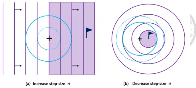
Figure 2.1: The one fifth rule of (1+1)-ES.

normal distribution as following:

x_i ∼ m + σNi(0, C),

where m ∈ R^d is the mean, σ ∈ R+ is the step-size, and C ∈ R^d^×d is the covariance matrix. The mean vector represents the positions where the best solution is most likely to appear. The step-size determines the area to search and modifies exploration and exploitation behaviors. The covaraince matrix determines the shape of the distribution ellipsoid.

2.1.1 (1+1)-ES

One of the simplest evolutionary strategy is (1+1)-ES. It samples one offspring x from parent m according to the equation described above. If the offspring x is better than m, it replaces m to be the new mean of the next sampling distribution. It also follows the one-fifth success rule as illustrated in Figure 2.1. The one-fifth success rule increases the step-size by 1.5 if the current sample is better than the previous best sample, i.e. the mean m. We believe the best solution, denoted as the flag in Figure 2.1(a), should be somewhere outside of our current distribution and we should increase step-size to explore more search space. The one-fifth success rule decreases the step-size by 1.5^−1/4 if the current sample is not better than the previous best sample. This means that we believe the best solution,

(21)

illustrated as the flag in Figure 2.1(b), should be within the sampling distribution, and we should decrease the step-size to further focus on the current region. Here we describe the (1+1)-ES with one-fifth success rule with independent restarts [1]. The pseudo code of (1+1)-ES is given in Algorithm 1.

Algorithm 1: (1+1)-ES with 1/5 success-rule

X_n: solution of the n^th iteration, σ_n: step size of the n^thiteration, N (0, I): multivariant normal distribution with mean vector 0 and identical covariance matrix I.

input : f : evaluation function output: X_n+1: best solution Initialize X₀, σ₀

while termination criterion not met do Xf_n= X_n+ σ_nN (0, I)

if f (X^f_n)≤ f(Xn) then X_n+1 =X^f_n

σ_n+1 = 1.5σ_n else

X_n+1 = X_n σ_n+1 = 1.5^−1/4σ_n return X_n+1

2.1.2 CMA-ES

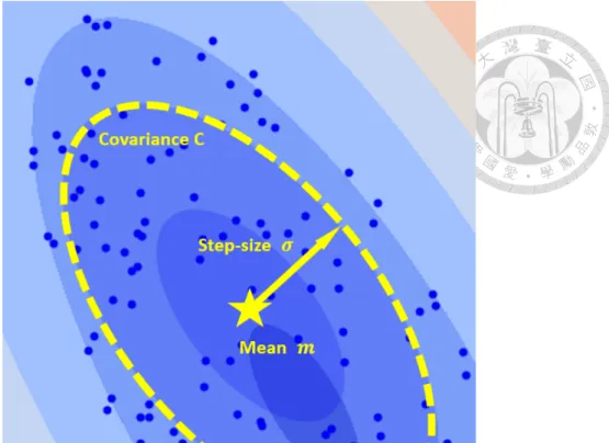
Covariance Matrix Adaptation Evolution Strategy (CMA-ES) is an evolutionary strategy proposed by Hansen in 2003 [7]. It adopts a multivariate normal distribution to generate isotropic search points which do not favor any direction. The multivariate normal dis- tribution is widely observed in the nature and relatively easy to design and analysis for algorithms. CMA-ES modifies three parameters to control the multivariate normal distri- bution: the mean m∈ R^d, the step-size σ∈ R+, and the covariance matrix C ∈ R^d^×d.

The mean indicates the translation of the normal distribution model. It indicates the most favorable position that should be sampled with the largest density. It is updated with the weighted mean of all the positions according to their fitness. The step-size controls the state of exploration or exploitation. An ideal step-size control gradually decreases the searching region for exploitation. One of the easiest step-size control method is the one-

(22)

Figure 2.2: Three major elements of CMA-ES.

fifth success rule, mentioned above. Later a cumulative step-size adaptation is proposed in Cumulative Step-size Adaptation Evolutionary Strategy (CSA-ES) [8], a predecessor of CMA-ES. The cumulative step-size adaptation measures the pathway of the mean vector in the generation sequence. Adapting the step-size according to the evolution path enables translating more efficiently to a desired location. Later, it also allows perpendicular around the desired region. The covariance matrix indicates the shape of the normal distribution model. Adapting the covariance matrix allows us to search in a region that is more coherent to the fitness landscape, This adaptation follows a natural gradient towards the direction of optimum solution. It can also learn a rotated representation of the problem and be coordinate independent. By adjusting these three parameters, shown in Figure 2.2, CMA- ES is extremely powerful on solving unimodal problems.

CMA-ES adopts a small population size to reduce function evaluations and increase the frequency of updating the underlying models. The default population size λ for a D-dimension problem, described in [6], is

λ = 4 +⌊3 log(D)⌋.

(23)

However, recent research suggest that it is benefitial to gradually increase the population size after random restart [2]. This parameter-less adaptation enables few evaluations consumption for easy problems, yet is also able to solve more difficult problems with a larger population size later.

2.2 Standard Particle Swarm Optimization

Particle Swarm Optimization (PSO) is a swarm intelligence optimization algorithm. It was first proposed by J. Kennedy and R. C. Eberhart in 1995 [11] to simulate the foraging behavior of bird flocks. The swarm is composed of particles that move around in a given multi-dimensional search space to find the best solution. Each particle updates its velocity according to its historical experience, as well as the information of the neighboring par- ticles. The neighborhood of a particle is a set of information links defined by the swarm topology. PSO iteratively updates the swarm topology, the velocities, and the positions of each particle until the global optimum solution is found.

Throughout the years, numerous variants of PSO have been proposed to improve per- formance. As a result, a standard PSO, composed of clear principals, is needed as the baseline for comparison. Standard PSO (SPSO) provides a well defined version that follows the common principals of PSO design. It is intended to be a milestone with simple and clear implementation for future comparison. So far, there have been three successive versions of standard PSO on the Particle Swarm Centeral¹: SPSO 2006, SPSO 2007, and SPSO 2011. The underlying principals of these three algorithms are generally the same as all PSO variants. The exact formula and implementation are slightly different due to latest theoretical progress. A detailed description of SPSO 2011 [23] is given in the following paragraphs.

1https://www.particleswarm.info/

(24)

2.2.1 Initialization of the swarm

For a search space E with a given dimension D, E is confined by a set of minimum and maximum bounds in each dimension. The hyperparallelepid search space E can be formally defined as the Euclidean product of D real intervals [4]:

E =

⊗D

d=1

[min_d, max_d].

For each position x within the multi-dimensional search space E, there exists a corre- sponding numerical value f (x), i.e. fitness. A swarm is composed of particles, which explore different positions in the search space to find the best corresponding fitness value.

At time t, each particle in the swarm possesses the following vectors with D coordinate:

• x_i(t) is the position of the particle i at time t.

• v_i(t) is the velocity of the particle i at time t.

• p_i(t) is the previous best position the particle i had been to, at time t.

• li(t) is the best position of all the previous best positions in the neighborhood of particle i at time t.

Let U (min_d, max_d) be a random number drawn from a uniform distribution within [min_d, max_d], and N_i(t) be a set of neighbors of particle i at time t defined by the swarm topology. In SPSO 2011 [4], each particle is initialized with a random position and velocity defined as following:

x_i(0) = U (min_d, max_d),

v_i(0) = U (min_d− xi,d(0), max_d− xi,d(0)), p_i(0) = x_i(0),

l_i(0) = argmin_j_∈N_i₍₀₎(f (p_j(0))).

(25)

The swarm size of SPSO 2011, denoted as S, is suggested as

S = 40,

yet it can also be defined by user [4].

2.2.2 Velocity update equations

Velocity update equations differs in different variations of PSO, since it is the core procedure of optimization that determines the performance of PSO. To prevent premature convergence, SPSO follows a random permutation order to update the positions of par- ticles in the swarm [4]. The position of particle i at time t + 1 depends on the previous position and the current velocity:

x_i(t + 1) = x_i(t) + v_i(t + 1).

The velocity of particle i at time t + 1 can be described as a combination of three vectors:

v_i(t + 1) = wv_i(t) + α(p_i(t)− xi(t)) + β(l_i(t)− xi(t)),

where w mimics the momentum of the particle, and α, β describes how successive actions are effected by the personal previous best position and the neighborhood previous best position.

In SPSO 2011, the velocity update equations eliminates the coordinate dependency by creating a hypersphere according to x_i, p_iand l_i, shown in Figure 2.3. The hypersphere is defined as:

H_i(G_i,||Gi− xi||),

with center G_iand radius||Gi−xi||. When the personal best pi(t) is not the neighborhood previous best l_i(t), the center G_i is defined as:

G_i = 1

3(x_i+ (x_i+ c(p_i− xi)) + (x_i+ c(l_i− xi))) = x_i+ c

3(p_i+ l_i− 2xi).

(26)

Figure 2.3: Velocity update of SPSO 2011.

If the personal best is the best in the neighborhood, i.e. p_i(t) = l_i(t), the center G_i is defined as:

G_i = 1

2(x_i+ (x_i+ c(p_i− xi))) = x_i+ c

2(p_i− xi).

In both cases, the acceleration constant c is:

c = 1

2+ ln(2)≃ 1.193.

As shown in Figure 2.3, a random sample x^′_iis drawn from the hypershpere with uniform random direction and uniform radius:

r = U (0,||Gi− xi||).

Therefore, the velocity update equation and new position of SPSO 2011 is defined as:

v_i(t + 1) = wv_i(t) + x^′_i(t)− xi(t),

x_i(t + 1) = x_i(t) + v_i(t + 1) = wv_i(t) + x^′_i(t),

(27)

Figure 2.4: Different topologies used by PSO.

where the inertia weight is also:

w = 1

2 ln(2) ≃ 0.721.

As mentioned before, the search space is defined as a hyperparallelepid with confine- ment [mind, maxd] in each dimension d. Therefore, after calculating the new velocities and positions of particles, we have to go through confinement check to make sure all particles stay inside the search space. There are multiple options to handle confinement in SPSO 2011. The following method described in [4] treat boundary as “wall”, so that all particles bounce back with half of previous velocity after they reach the border. For the new position x_i,d(t + 1) of particle i in dimension d,

if (x_i,d(t + 1) < min_d), x_i,d(t + 1) = min_d,

v_i,d(t + 1) =−0.5vi,d(t + 1).

if (x_i,d(t + 1) > min_d), x_i,d(t + 1) = max_d,

v_i,d(t + 1) =−0.5vi,d(t + 1).

2.2.3 The adaptive random topology

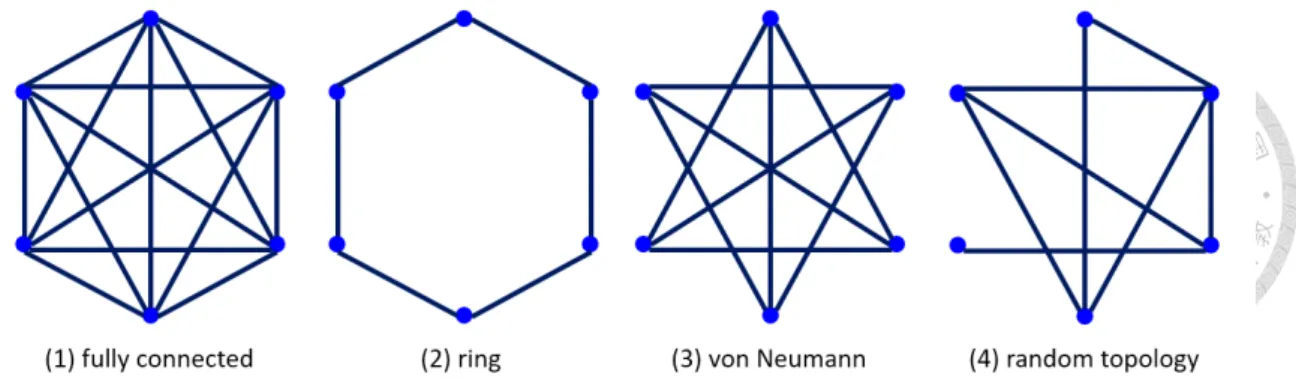
The swarm topology defines “who informs whom” to help distribute the information of optimum solution in the swarm. Multiple topologies shown in Figure 2.4 are adopted in different version of PSO. The random topology adopted in SPSO 2011 is updated under

(28)

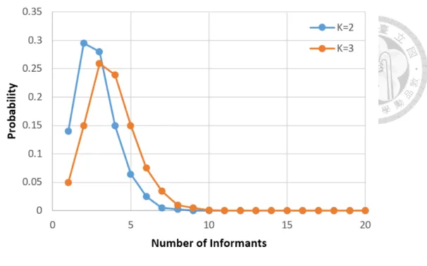
Figure 2.5: Probability of different numbers of informants in the random topology.

two circumstances [4]:

• at the very beginning

• after an iteration with no improvement of the best known fitness value

For each particle p_i in a swarm of n particles S = {p1, p₂, ..., p_n}, a good topology should allow each p_ito inform itself, along with a set of randomly selected particles from the other n− 1 particles [3]. We would like most of the particles to be informed by two to four particles in the topology. Some of the particles can have no informant except for itself. There should also exist a non-zero probability for a particle to be informed by all the other particles.

In order to construct a random topology that satisfy the desirable features mentioned above, Clerc proposed a method [3] that results in a distribution of the sum of n − 1 independent binary Bernoulli variables, shown in Figure 2.5. We use the distribution K = 3, meaning that each particle tells three other particles about their previous best fitness and position.

(29)

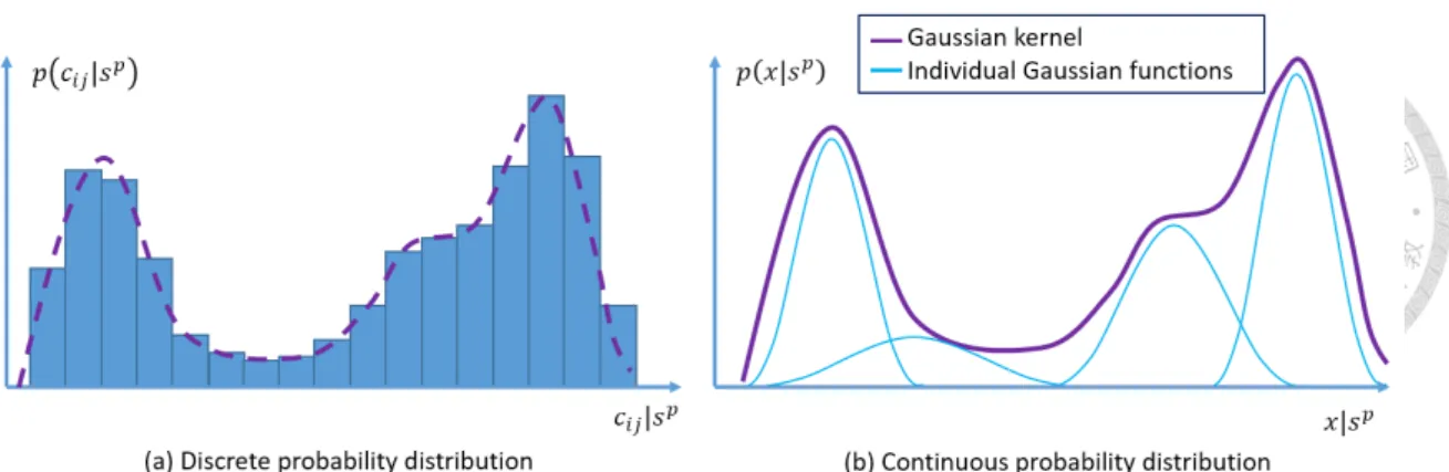
Figure 2.6: Comparison of discrete PDF continuous Gaussian kernel PDF.

2.3 Ant Colony Optimization for Continuous Domain

Ant Colony optimization (ACO) is first proposed by Dorigo [5] to solve combinatorial optimization problems, including scheduling, routing, and timetabling. These problems aim to find optimal combinations or permutations of finite sets of available components.

Inspired by the foraging behavior of natural ants, ACO mimics the pheromone deposition of ants along the trail to a food source. The deposited pheromone, which indicates the quantity and quality of the food, creates an indirect communication among ants and en- ables them to find the shortest paths. Two major procedures: solution construction and pheromone update, are detailed in the following paragraph.

2.3.1 Discrete solution construction and pheromone update

For solution construction, we first consider a search space S defined over a finite set of all possible solution components, denoted by C. Each solution component, denoted by c_ij, is a decision variable Xiinstantiated with value v_i^j ∈ Di ={vi¹, ..., v_i^|Dⁱ^|}. To construct a new solution, an artificial ants starts with an empty partial solution s^p =∅. During each construction step, the partial solution s^p is extended with a feasible solution from the set N (s^p) ∈ C \ s^p. The probabilistic pheromone model adopted for selecting a feasible solution from N (s^p) can be defined as follows:

p(c_ij|s^p) = τ_ij^α· η(cij)^β

∑

ciℓ∈N(s^p)τ_iℓ^α· η(ciℓ)^β,∀cij ∈ N(s^p),

(30)

where τij is the pheromone value associated with component cij, and η(·) is a weight- ing function. α and β are positive parameters which determine the relation between pheromone and heuristic information.

The pheromone update, also known as pheromone evaporation, acts as solution se- lection. It increases the pheromone values associated with promising solutions and decreases the pheromone values associated to the bad ones. This is achieved by increasing the pheromone levels of more preferred solutions by ∆τ . Let ρ∈ (0, 1] be the evaporation rate. If the pheromone value is associated with a chosen good solution s_ch, the pheromone value is updated as following:

τ_ij = (1− ρ)τij + ρ∆τ,

while the other unrelated pheromone values are updated as:

τ_ij = (1− ρ)τij.

Thus, the discrete pheromone model shown in Figure 2.6(a) can be updated to emphasize the good solutions.

2.3.2 Continuous solution construction and phermone update

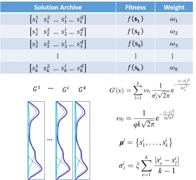
Over the years, multiple approaches of extending the ACO on continuous domain have been given. One of the most successful version is ACO_R, proposed by Socha and Dorigo in 2008 [18]. It extends ACO to the continuous domain without making any major con- ceptual change to its structure. The fundamental idea underlying ACORis to substitute the discrete probability distribution with a continuous PDF in each dimension, demonstrated in Figure 2.6. ACO_Rkeeps a solution archive of top-k solutions it has seen so far, shown in Figure 2.7. All the solutions are sorted(ties are broken randomly) according to their fit- ness f (s), so that the best solution stays at the top of the archive. For the i-th dimension, a Gaussian kernel PDF Gⁱ(x) is constructed with multiple weighted normal distributions

(31)

Figure 2.7: The solution archieve of ACO_R

(32)

g_jⁱ(x):

Gⁱ(x) =

∑k

j=1

ω_ℓg_ℓⁱ(x) =

∑k

ℓ=1

ω_ℓ 1 σⁱ_ℓ√

2πe⁻

(x−µi)2 2σiℓ

2 .

Such a PDF is easy to sample and provides a better flexibility to describe the landscape.

Three elements decide the shape of the Gaussian kernel:

• ωℓ is the weight of the solution sℓ.

• µⁱ is i-th value of all the solutions in the archive.

• σⁱ is standard deviation that determines that new samples.

Following are some parameters used by ACORthat also effects the Gaussian kernel con- struction. k is the size of the solution archive, which works like the memory of the swarm.

It may not be smaller than the number of dimensions. q represents the locality of the search process, i.e. how often should we not pick the best solution in the archive. It controls ex- ploration so that give a higher value of q leads to slower yet more robust convergence.

ξ > 0 represents the speed of convergence that has effect similar to the pheromone evapo- ration rate in ACO. It works like selection and enhance the good solutions in the archive.

The initial solution construction process proceed as following. After evaluating k randomly generates solutions, they are stored along with their fitnesses and weights in the solution archive. The weights are calculated according to the equation in Figure 2.7. Then the solution archive is sorted horizontally according to the fitness so that the best solution s₁is on the top

For general solution construction, we first define m as the number of ants used in an iteration for sampling. During each iteration, m new solutions are constructed dimension by dimension by sampling the i-th dimension Gaussian kernel Gⁱ A more detailed and efficient process of sampling the Gaussian kernel PDF is described in [18].

Pheromone update is accomplished by adding the new samples, their fitness, and the corresponding weight into the archive. Then, the solution archive is sorted according to the fitness and we only keep the top-k solutions in the archive. This selection process ensures only the best solutions are kept in the archive. Therefore, future samples will be constructed near these best solutions and guide the ants toward the optimum.

(33)

Chapter 3 Clustering Techniques

We are interested in solving real-valued multimodal problems composed of observable unimodals. Given the case, it is easier to solve an isolated unimodal within a subspace, than tackling the complete search space with the multimodal problem. Therefore, the first thing for solving a multimodal problem is to identify and isolate the potential unimodals within the given search space.

We tried to isolate potential fitness hills, i.e. unimodals, by clustering the initial sam- ples points, and consider each cluster as a multi-dimension normal distribution. Differ- ent clustering techniques are often applied to identify different characteristics of clusters.

Here we proposed a hierarchical clustering techniques to identify fitness hills, since we consider not only the density of the particles, but also the fitness values of different search points. Our basic assumption for the under lying unimodal is a weighted normal distribution, since we need to take fitness into account instead of viewing each point with the same weight. We tend to focus on the particles with better fitness, than a dense cluster with less fitness. It is also easier to calculate the weighted mean vector and weighted covariance matrix in higher dimension.

Later, we applied the Minimum Description Length (MDL) to reduce the number of clusters. Although a complex Gaussian Mixture Modal is able to describe the sample distribution better, we believe that a more compact model, in terms of information entropy, is the better choice when multiple models can describe the same distribution. This also allows us to define a more stable subspace for further searching.

(34)

3.1 K-Means Clustering

In this section, we first describe the K-Means clustering techniques and its limitation for identifying the fitness hills. K-Means clustering aims to partition n observation data points into k clusters. There are two main procedures for K-Means clustering: the assignment step and the update step.

During the assignment step, an initial set of k means positions are given. Then, each data point is assigned to the cluster with the nearest mean. The assignment to the nearest mean can be formally described as creating clusters whose mean yields the least within- cluster sum of squares (WCSS), textiti.e. the sum of squared Euclidean distance. During the update step, the new centroids of each new clusters are calculated and assigned as the new means. This can be also be described as minimizing the WCSS. The algorithm pro- ceeds by alternating between these two steps until the means no longer change. Since there only exists a finite states of partitions, the algorithm must converge to a local optimum.

However, different initial mean positions results in different clusters.

One of the main problem for using the K-Means clustering to identify fitness hills is that it considers only the spatial density and does not utilize the fitness value of each parti- cle. Different sets of initial centers might result in different kinds of clusters. Meanwhile, each cluster might be centering at a point that does not necessarily possess the best fitness in the neighborhood. Therefore, the K-Means clustering often results in unstable clus- ters depending on initial conditions, and is highly sensitive to particle density. Another common phenomenon for being sensitive to spatial density is that the points on the border of clusters might belong to different clusters after each update. This makes the clusters unstable and costs unnecessary evaluations and computation for redefining the borders of ROI after each update.

The other problem for using the K-Means clustering is that one needs to decide the number of clusters. Determining the number of clusters is also a highly studied subjects.

We briefly discuss three common estimation methods that we have tried, the silhouette coefficient [17] , the gap statistics [20] , and the Hartigans’ dip test [9] in the following paragraph.

(35)

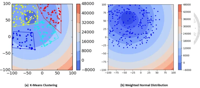
Figure 3.1: Comparing K-Means clustering with weighted Gaussian Distribution on CEC2005 F1 Problem

The silhouette coefficient measures how cohesive an object is to its own cluster and how separated it is to the other clusters. Ranging from -1 to 1, the silhouette coefficient with a higher value indicates it is more likely to belong to its own cluster. The gap statistics compares the change in within-cluster dispersion with that of an reference null distribution. It calculates the gap statistics for different number of clusters and select the one with the maximum gap statistics. The Hartigans’ dip test uses the empirical cumulative distribution function (ECDF) to measure the maximum difference between multimodal samples and the unimodal samples. It calculates maximum deviation of the sample ECDF from the unimodal CDF and check if the difference is statistically significant.

We desire that as the algorithms proceed, particles should gather around the good solutions and gives a clear density signal. However, they seldom identify a unimodal at the beginning. It means that we need to add up more particles to meet the population size re- quirement for each clusters. This increases the density in that specific region, and creates an artificial cluster that should not exist in the first place.

Figure 3.1 shows how K-Means fails to identify a unimodal and results in four clusters due to density. A more preferable clustering result is shown on the right in Figure 3.1. We would like our clustering method to be capable of identifying the unimodal and be able to center around the particle with the best fitness.

(36)

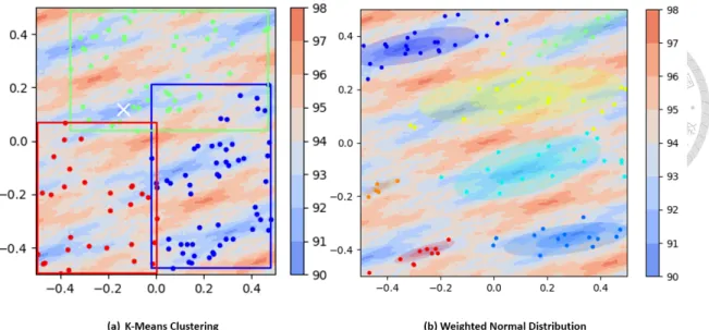
Figure 3.2: Comparing K-Means clustering with weighted Gaussian Distribution on CEC2005 F11 Problem

Figure 3.2 shows another example of how K-Means fails to identify the right multi- modals. Since K-Means only consider the density, it is hard to recognize the dense hills in the landscape. This initial clusters leads to more unnecessary evaluations for merging and re-identifying the hills. However, we can see that on the right, our technique successfully recognize almost all the hills in the problem. It also helps to locate the local optimum solutions approximately at the center. This gives lost of advantages for the algorithms to search, since the task becomes exploiting a single hill. Therefore, later we adopted the weighted normal distribution as the underlying model.

3.2 Heirarchical Clustering

Since we would like to recognize the fitness hills, we modified the agglomerative cluster- ing technique to create hierarchical clusters. For a problem in D dimension, we defined the neighborhood of a particle to be the 4 +⌊3 log(D)⌋ particles with the minimum Eu- clidean distance, including the particle itself. Given the neighborhood of each particle, we create a directed graph by pointing each particle to the particle with the highest fitness in the neighborhood. If a particle does not possess the best fitness in its neighborhood, it points toward the direction with the maximum gradient. If it is the best particle in the

(37)

Figure 3.3: Before and after applying Minimal Description Length on CEC2005 F19 Prob- lem

neighborhood, it is very likely to be at the approximate location of local minimum.

We then create trees with the directed graph, where each tree represents a cluster with a potential fitness hill. The best position within this cluster is indicated by the root node.

This way, the fitness signal guides the construction of clusters, so that this method is able to identify more fitness hills than the K-Means clustering. Moreover, we do not need to provide the estimate number of clusters, since the agglomerative clustering method in- trinsically identifies fitness hills. These characteristics solves some fundamental problems that we faced when using the K-Means clustering along with different number-of-clusters- estimation techniques.

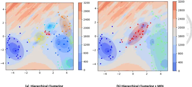
We can see that for a multimodal problem depicted in Figure 3.3(a), the hierarchical clustering technique successfully identifies several fitness hills. However, for the unimodal problem in Figure 3.4(a), the hierarchical clustering creates multiple “ripples” on the marginal area. These clusters are created when the best particle is a bit further from the next best particle. This indicates that the using the Euclidean distance as the distance metric is not suitable for problems with larger hills.

In order to solve this problem, we assume the underlying hills are composed of multivariate normal distribution. Given the distribution and a sample position, we can use the Manhanoblis distance to serve as a more expressive metric. We would also like to

(38)

Figure 3.4: Before and after applying Minimal Description Length on CEC2005 F1 Prob- lem

determine the number of clusters in the beginning, since we believe that the problems are composed of hierarchical hills. We do not need to invest so much resources in so many regions during the initialization. Reclustering after a few iterations shall give us a better signal about where to focus.

3.3 Minimum Description Length

The Minimum Description Length (MDL) principle was introduced by Rissanen in 1978 [14].

It adopts the idea of Occams’s razor by selecting the codec that gives the shortest code length of the data. It provides a natural safeguard against overfitting, since it considers not only the goodness of the model, but also the complexity of the data to give the hy- pothesis. Here we modified the MDL described in [12] to help us determine the optimum number of clusters that provides the most efficient codes for the sample data. The MDL considers both data description accuracy and model description efficiency.

3.3.1 Data description accuracy

Since we would like to take the fitness into account, we use the weighted Gaussian dis- tribution as the underlying model. For a cluster with N particles, each particle X_i has a rank r_i between 1 and N (ties are broken randomly) that corresponds to the fitness. The

(39)

weight ωican be defined as:

ω_i = log(N + 0.5)− log(ri). (3.1)

The mean µ and covariance matrix Σ in a weighted Gaussian distribution N can be denoted as:

µ = 1

∑_N

i=1ω_i

∑N

i=1

ω_iX_i, (3.2)

Σ = 1

∑_N

i=1ω_i

∑N

i=1

ω_i(X_i − µ)^T(X_i− µ). (3.3)

Let X = {X1, X₂, ..., X_I} denote the data set, composed of I samples. Each sam- ple is a D-dimensional vector X_i = {Xi1, ..., X_iD}. The class-probability of observing sample X_i in class j, described by a parameter set Θ_j, can be denoted as P_j(X_i|Θj). The probability of observing the sample X_i in a finite mixture model with J components can be denoted as:

P (Xi|Θ) =^∑^J

j=1

αjPj(Xi|Θj), (3.4)

αj = nj/I, (3.5)

where αj is the prior probability that Xi belongs to the j-th model, and nj denotes the number of samples in cluster j.

Therefore, the probability of observing sample X_iin cluster j can be further described by the j-th weighted Gaussain distribution:

P (X_i|Θj) = N (X_i|µj, Σ_j). (3.6)

With the assumption that the data instance X_iare independently distributed, the joint data probability is the product of the individual instance probabilities:

P (X|Θ) = ^∏^I

i=1

∑J

j=1

α_jP_j(X_i|Θj). (3.7)

However, we would like to give a higher weight for the data with better fitness. The

(40)

weight for Xij, the i-th particle that belongs to the j-th model with rank rij within the j-th cluster, is:

ω_ij = log(n_j + 0.5)− log(rij), (3.8) and the normalized weight is:

w_ij = ω_ij

∑nj

i=1ωij

, (3.9)

the data description accuracy can be descrived as a weighted sum of individual log-likelihoods:

log(P (X|Θ)) =^∑^J

j=1

(nj(log(αj) +

nj

∑

i=1

wijlog(Pj(Xij|Θj)))). (3.10)

3.3.2 Model description efficiency

Although a more complex model can describe the data distribution better, we believe that a simpler model with approximately the same accuracy is better. Therefore, the number of parameters that a model requires, is also considered in MDL. The free parameters in the Gaussian mixture model are:

• J − 1 paramters for J weights αj, since^∑α_j = 1

• D parameters for each mean µ_j

• D(D + 1)/2 parameters for each covariance matrix Σ_j

Therefore, the total number of free parameters is

K = J − 1 + J(D + D(D + 1)/2) = J(D²+ 3D + 2)/2− 1. (3.11)

Combining the data description accuracy and model description efficiency, the MDL defined in [15] is denoted as:

minK,Θ − log(P (X|Θ)) + 1

2K log(I). (3.12)

(41)

3.3.3 Model selection with MDL

As mentioned before, we need to solve the problem of having too many “ripple” clusters on the margin area. Here we would like to use the MDL Equation to calculate model efficiency, and merge overfitting clusters. Therefore, after identifying potential unimodals with hierarchical clustering in Section 3.2, we use Equation 3.3.2 to calculate model efficiency. We created multiple weighted Gaussian distribution according to the hierarchical clusters, as shown in Figure 3.4(a) and 3.3(a). Then we try all combinations of merging two clusters and calculate the corresponding MDL. Therefore, we compare the MDL score between the original hierarchical clusters and the new clusters with the minimal MDL score. If the MDL score of the new model is smaller than the previous model, we repeat the same procedure and keep merging. This procedure terminates when there is only one cluster remain, or when the minimum MDL score of all possible new modals is larger than the MDL score of the previous model. Then we get fewer yet still expressive clusters, shown in Figure 3.4(b) and 3.3(b).

(42)

(43)

Chapter 4 Linear Projection

In this chapter, the technique of defining a region of interest that contains only one uni- model for exploitation. Also, some algorithms, e.g. SPSO, requires a well-defined hyper- cube search space with fixed-value constraints in each dimension. Defining the projection onto subspace can be described as a model selection. In our case, this process does not require high accuracy, yet has a strict demand on time consumption. Combining the re- quirements, we use a linear projection matrix to project the original search space onto a subspace with feasible solutions bounded within [0, 1] in each dimension.

One of the advantage for using projection matrix is that for a problem with ℓ variables, a linear projection matrix on homogeneous coordinate only requires (ℓ + 1)²hyperparameters to be optimized. Therefore, less hyperparameters are assigned than directly define each hyperplane borders or vertices. This reduces the parameters that we need to optimize and results in less time consumption during model selection. We also use the (1+1)-ES, a fast and simple evolutionary strategy, to optimize the matrix. It allows us to rapidly approximate a high dimensional projection matrix within given number of iterations.

Furthermore, subspace projection also gives advantage for solving inseparable prob- lems. For variables that are not independent, projection allows the algorithm to solve an easier, rotated and sheared problem on subspace, as shown in Figure 4.1. The homogeneous projection matrix separates the original ROI into less overlapped ROI, which reduces redundant search and sometimes enlarges the crucial regions.

In the following sections, we first describe the canonical affine transformation. Then

(44)

Figure 4.1: Projecting inseparable problems onto subspace.

we discuss how the projection matrix allows linear projection in a homogeneous coordinate. Finally, we give details of how we design the cost function and how we utilize the (1+1)-ES to optimize the projection matrix.

4.1 Affine Transformation

In geometry, an affine transformation preserves points, straight lines and planes. For two affine spaces A and B and any pair of points P, Q∈ A, an affine transformation f deter- mines a linear transformation φ that can formally defined as:

−−−−−−→

f (P )f (Q) = φ−−−→

(P Q).

Here, we list some common 2D affine transformation matrix in Figure 4.2.

1. Translation

Translation moves every point in the cluster by the same amount in a given direction.

It allows us to reallocate the center of ROI to the positions with the best fitness.

2. Rotation

(45)

Figure 4.2: Some common affine transformation

(46)

Rotation is a common method to make a problem inseparable, by creating depen- dencies among variables. Therefore, using a rotation matrix to rotate the problem allows us to alter the problem characteristics. In higher dimensions, rotating about different axis requires different form of matrix. Here we only demonstrate a simple two dimensional case in Figure 4.2.

3. Scaling

Scaling transformation can stretch or shrink a given search space. Since it changes the lengths and angles, scaling is not an Euclidean transformation. In search space projection, it allows us to enlarge certain areas that we are interested in, and shink some area that we tend to ignore on the subspace.

4. Shearing

Shearing transform acts like “pushing” the search space in a direction parallel to a certain plane or axis. It changes the lengths and angles of certain area on the subspace. This transformation also allows us to expend certain interesting areas on subspace for a more thorough search.

Figure 4.3: General affine transformation in 2D

The general affine transformation can be expressed as the form in Figure 4.3. All the common affine transformation matrix mentioned above, including translation, rotation, scaling and shearing can fit into this form. The general affine transformation can be seen

(47)

Figure 4.4: Affine transformation and projective transformation comparison.

as the matrix product of several affine transformation matrices. Although the affine transformation does not preserve the lengths and angles of certain shape, it does not alter the degree of a polynomial. That means parallel lines and planes are transformed to parallel lines and planes, and intersecting lines and planes are also transformed into intersecting lines and planes. It preserved certain geometric characteristics, which is beneficial for us to do searching on subspace.

However, the affine transformation can only create a hyperparallelepid ROI, as shown in Figure 4.4 The parallelogram shape is sometimes not flexible enough to define a non- overlapping ROI that matches the shape of the fitness landscape. In order to acquire a more flexible quadrilateral ROI, we need the projective transformation. Projective transformation is more expressive than affine transformation since the last row does not have to be 0, 0, and 1.

4.2 Projective Transformation

Projective transformations are the most general linear transformations and require the use of homogeneous coordinates. The homogeneous coordinate is also called projective coor- dinates, since it is a system of coordinates widely adopted in projective geometry. Given

(48)

Figure 4.5: Projective transformation matrix.

Figure 4.6: Comparison between inverse affine transform and inverse projective transformation.

a point (x, y) on the Euclidean plane, than (xZ, yZ, Z) is called a set of homogeneous coordinates for the point, for any non-zero real number Z. One of the great advantage of homogeneous coordinate is that the points, including the ones at infinity, can be repre- sented with simpler, finite coordinates. That is, when Z is 0, the homogeneous coordinates of the point is defined at infinity.

Therefore, as shown in Figure 4.5, for given a position (x, y) on the original search space, we get a projected homogeneous coordinate (x^′′, y^′′) on the subsapce. We can generalize this to any d-dimensional space. The homogeneous convention is to convert the projected position, a vector with (d + 1) variables, to a d variable vector by dividing first d elements with the last element.

However, unlike the affine transformation, the projective transformation does not guarantee inverse transform. The projection matrix does not guarantee a non-zero matrix de-