Comparison of Discrimination Methods for the Classi’ cation of Tumors Using Gene Expression Data
Sandrine Dudoit, Jane Fridlyand, and Terence P. Speed
A reliable and precise classi cation of tumors is essential for successful diagnosis and treatment of cancer. cDNA microarrays and high- density oligonucleotide chips are novel biotechnologies increasingly used in cancer research. By allowing the monitoring of expression levels in cells for thousands of genes simultaneously, microarray experiments may lead to a more complete understanding of the molecular variations among tumors and hence to a ner and more informative classi cation. The ability to successfully distinguish between tumor classes (already known or yet to be discovered) using gene expression data is an important aspect of this novel approach to cancer classi cation. This article compares the performance of different discrimination methods for the classi cation of tumors based on gene expression data. The methods include nearest-neighbor classi ers, linear discriminant analysis, and classi cation trees. Recent machine learning approaches, such as bagging and boosting, are also considered. The discrimination methods are applied to datasets from three recently published cancer gene expression studies.
KEY WORDS: Cancer; Discriminant analysis; Microarray experiment; Supervised learning; Tumor classi cation; Variable selection.
1. INTRODUCTION
A reliable and precise classi cation of tumors is essen- tial for successful diagnosis and treatment of cancer. Current methods for classifying human malignancies rely on a variety of morphological, clinical, and molecular variables. Despite recent progress, there are still uncertainties in diagnosis. Fur- thermore, it is likely that the existing classes are heterogeneous and comprise diseases that are molecularly distinct and follow different clinical courses. cDNA microarrays and high-density oligonucleotide chips are novel biotechnologies increasingly used in cancer research (Alon et al. 1999; Golub et al. 1999;
Perou et al. 1999; Pollack et al. 1999; Alizadeh et al. 2000;
Ross et al. 2000). By allowing the monitoring of expression levels in cells for thousands of genes simultaneously, microar- ray experiments may lead to a more complete understanding of the molecular variations among tumors and hence to a ner and more reliable classi cation.
Types of microarray systems include the cDNA microarrays developed in the Brown and Botstein labs at Stanford (DeRisi, Iyer, and Brown 1997; Eisen, Spellman, Brown, and Bot- stein 1998) and the high-density oligonucleotide chips from the Affymetrix Company (Lockhart et al. 1996); the brief description here focuses on the former. cDNA microarrays consist of thousands of individual DNA sequences printed in a high-density array on a glass microscope slide using a robotic arrayer. The relative abundance of these spotted DNA
Sandrine Dudoit is Assistant Professor, Division of Biostatistics, Uni- versity of California, Berkeley, Berkeley, CA 94720 (E-mail: san- [email protected]). Jane Fridlyand is a Postdoctoral Scientist at the UCSF Cancer Center, San Francisco, CA 94143 (E-mail: [email protected]).
Terence P. Speed is Professor, Department of Statistics, University of Cali- fornia, Berkeley, Berkeley, CA 94720 (E-mail: [email protected]). This work was supported in part by an MSRI postdoctoral fellowship, a PMMB Burroughs–Wellcome fellowship, and by National Institutes of Health grant R01GM59506 (TPS). The authors are grateful to Ash Alizadeh, Pat Brown, Mike Eisen, and Doug Ross for providing access to their data. Pablo Tamayo’s assistance with the ALL/AML data is greatly appreciated. Finally, the authors thank Leo Breiman, Yoram Gat, David Nelson, Mark van der Laan, and Yee Hwa Yang for many helpful discussions and suggestions, Sam Buttrey for his nearest-neighbor program, and the referees for their comments on an ear- lier version of this article. Supplementary analyses and gures are available at http://www.stat.berkeley.edu/users/terry/zarray/html. Dudoit and Fridlyand contributed equally to this work.
sequences in two DNA or RNA samples may be assessed by monitoring the differential hybridization of the two samples to the sequences on the array. For mRNA samples, the two samples, or targets, are reverse-transcribed into cDNA, labeled using different uorescent dyes [e.g., a red uorescent dye (cyanine 5 or Cy5), and a green uorescent dye (cyanine 3 or Cy3)], then mixed in equal proportions and hybridized with the arrayed DNA sequences, or probes (following the def- inition of probe and target adopted in The Chipping Fore- cast 1999). After this competitive hybridization, the slides are imaged using a scanner and uorescence measurements are made separately for each dye at each spot on the array. The ratio of the red and green uorescence intensities for each spot is indicative of the relative abundance of the corresponding DNA probe in the two nucleic acid target samples. (See The Chipping Forecast 1999 for a more detailed introduction to the biology and technology of cDNA microarrays and oligonu- cleotide chips.)
Microarray experiments raise numerous statistical questions in elds as diverse as image analysis, experimental design, cluster and discriminant analysis, and multiple hypothesis test- ing. Here we focus on the classi cation of tumors using gene expression data. Three main types of statistical problems are associated with tumor classi cation: (a) identi cation of new tumor classes using gene expression pro les, cluster analy- sis/unsupervised learning; (b) classi cation of malignancies into known classes, discriminant analysis/supervised learning;
and (c) identi cation of “marker” genes that characterize the different tumor classes, variable selection. Data from these new types of experiments present a “large p, small n” prob- lem; that is, a very large number of variables (genes) relative to the number of observations (tumor samples). The publicly available datasets typically contain expression data on 5,000–
10,000 genes for less than 100 tumor samples. Both numbers are expected to grow, the number of genes reaching on the order of 30,000, an estimate for the total number of genes in the human genome.
© 2002 American Statistical Association
Journal of the American Statistical Association
March 2002, Vol. 97, No. 457, Applications and Case Studies
77
Recent publications on cancer classi cation using gene expression data have focused mainly on the cluster analysis of both tumor samples and genes and include applications of hierarchical clustering (Alon et al. 1999; Perou et al. 1999;
Pollack et al. 1999; Alizadeh et al. 2000; Ross et al. 2000) and partitioning methods such as self-organizing maps (Golub et al. 1999). Alizadeh et al. (2000) used hierarchical clus- tering to study gene expression in the three most prevalent adult lymphoid malignancies. Ross et al. (2000) also relied on hierarchical clustering to monitor gene expression in the 60 cell lines from the National Cancer Institute’s anticancer drug screen. Using acute leukemias as a test case, Golub et al.
(1999) explored both the cluster analysis and the discriminant analysis of tumors using gene expression data. For discrimi- nant analysis, or “class prediction,” they proposed a “weighted gene voting scheme” that turns out to be a variant of a spe- cial case of linear discriminant analysis (Section 2.2). So far, most published articles on tumor classi cation have applied a single technique to a single gene expression dataset, and it is hard to assess the merits of each method in the absence of a comprehensive comparative study.
This article compares the performance of different discrim- ination methods for the classi cation of tumors based on gene expression pro les. These methods include traditional ones, such as nearest-neighbor and linear discriminant analysis, as well as more modern ones, such as classi cation trees. Recent machine learning approaches, such as bagging and boosting, are also considered. The discrimination methods are applied to three recently published datasets: the leukemia (ALL/AML) dataset of Golub et al. (1999), the lymphoma dataset of Alizadeh et al. (2000), and the 60 cancer cell line (NC I 60) dataset of Ross et al. (2000). The article is organized as fol- lows. Section 2 discusses the discrimination methods consid- ered in the comparision study. The datasets are described in Section 3, along with preliminary data processing steps. The study design for the comparison of the discrimination meth- ods is discussed in Section 4, and the results of the study are presented in Section 5. Finally, our ndings are summarized and open questions outlined in Section 6.
2. DISCRIMINATION METHODS
For our purposes, gene expression data on p genes for n tumor mRNA samples may be summarized by an n p matrix X D 4x
ij5, where x
ijdenotes the expression level of gene (vari- able) j in mRNA sample (observation) i. The expression lev- els might be either absolute (e.g., oligonucleotide arrays used to produce the leukemia dataset) or relative to the expres- sion levels of a suitably de ned common reference sample (e.g., cDNA microarrays used to produce the lymphoma and NC I 60 datasets). When the mRNA samples belong to known classes (e.g., follicular lymphoma), the data for each observa- tion consist of a gene expression pro le x
iD 4x
i11 : : : 1 x
ip5 and a class label y
i, that is, of predictor variables x
iand response y
i. For K tumor classes, the class labels y
iare de ned to be integers ranging from 1 to K, and n
kdenotes the number of observations belonging to class k. Note that the expres- sion levels x
ijare in general highly processed data; the raw data in a microarray experiment consist of image les, and important preprocessing steps include image analysis of these
scanned images and normalization. In addition, for the pub- licly available datasets, the number of tumors n is typically below 100, whereas the number of genes p is several thou- sands. In the comparison of prediction methods, the number of genes will be substantially reduced by identifying a subset of genes whose expression levels are associated with tumor class (Section 3.4).
A predictor or classi er for K tumor classes partitions the space ¸ of gene expression pro les into K disjoint and exhaustive subsets, A
11 : : : 1 A
K, such that for a sample with expression pro le x D 4x
11 : : : 1 x
p5 2 A
k1 the predicted class is k. Predictors are built from past experience, that is, from tumor samples known to belong to certain classes. Such observations comprise the learning set (LS), ¬ D 84x
11 y
151 : : : 1 4x
nL1 y
nL59.
Predictors may then be applied to a test set (TS), ´ D 8x
11 : : : 1 x
nT9, to predict the class y
i. expression pro le x
iin the test set for each gene. In the event that the y
iare known for the test set, the predicted and true classes may be com- pared to estimate the error rate of the predictor. A classi er built from a learning set ¬ is denoted by £4¢1 ¬5; the pre- dicted class for a tumor sample with gene expression pro le x is £4x1 ¬5. Here, we review brie y a number of well-known discrimination methods. General references on discriminant analysis include works by Mardia, Kent, and Bibby (1979), McLachlan (1992), and Ripley (1996).
2.1 Fisher Linear Discriminant Analysis
First applied by Barnard (1935) at the suggestion of Fisher (1936), Fisher linear discriminant analysis (FLDA) is based on nding linear combinations xa of the gene expression lev- els x D 4x
11 : : : 1 x
p5 with large ratios of between-group to within-group sums of squares. (See Mardia et al. 1979 for a detailed presentation of FLDA.) For an n p learning set data matrix X, the linear combination Xa of the columns of X has a ratio of between-group to within-group sums of squares given by a
0Ba=a
0W a, where B and W denote the p p matrices of between-group and within-group sums of squares and cross-products. The extreme values of a
0Ba=a
0W a are obtained from the eigenvalues and eigenvectors of W
ƒ1B. The matrix W
ƒ1B has at most s D min4K ƒ11 p5 nonzero eigenval- ues, ‹
1¶ ‹
2¶ ¢ ¢ ¢ ¶ ‹
s, with corresponding linearly indepen- dent eigenvectors v
11 v
21 : : : 1 v
s. The discriminant variables are de ned as u
lD xv
l1 l D 11 : : : 1 s, and in particular, a D v
1maximizes a
0Ba=a
0W a.
For a tumor sample with gene expression pro le x D 4x
11 : : : 1 x
p5, let d
k4x5 D P
slD1
44x ƒ Nx
k5v
l5
2denote its (squared) Euclidean distance, in terms of the discriminant variables, from the 1 p vector of class k sample means Nx
kD 4 Nx
k11 : : : 1 Nx
kp5 for the learning set ¬. The predicted class for gene expression pro le x is the class whose mean vector Nx
k, is closest to x in the space of discriminant variables, that is,
£4x1 ¬5 D arg min
kd
k4x50 FLDA is a nonparametric method
which also arises in a parametric setting. For K D 2 classes,
FLDA yields the same classi er as the sample maximum like-
lihood discriminant rule for multivariate normal class densities
with the same covariance matrix (see Section 2.2, case 1 for
K D 2).
2.2 Maximum Likelihood Discriminant Rules
In a situation where the tumor class conditional densities, pr4x—y D k5, are known, the maximum likelihood 4ML5 dis- criminant rule predicts the class of a gene expression pro le x D 4x
11 : : : 1 x
p5 by that which gives the largest likelihood to x, that is, £4x5 D arg max
kpr4x—y D k5. When the class- conditional densities are fully known, a learning set is not needed, and the classi er is simply £4x5. In practice, however, even if the parametric form of the class conditional densities is known, the parameters must be estimated from a learning set.
Using parameter estimates in place of the unknown parameters yields the sample ML discriminant rule.
For multivariate normal class densities, that is, for x—y D k N 4Œ
k1 è
k5, the ML discriminant rule is £4x5 D arg min
k84x ƒ Œ
k5è
ƒ1k4x ƒŒ
k5
0Clog—è
k—9. In general, this is a quadratic dis- criminant rule. Interesting special cases include:
1. Linear discriminant analysis (LDA). When the class den- sities have the same covariance matrix, è
kD è, the discriminant rule is based on the square of the Maha- lanobis distance and is linear in x, and given by £4x5 D arg min
k4x ƒ Œ
k5è
ƒ14x ƒ Œ
k5
00
2. Diagonal quadratic discriminant analysis (DQDA).
When the class densities have diagonal covariance matri- ces, ã
kD diag4‘
k121 : : : 1‘
kp25, the discriminant rule is given by additive quadratic contributions from each gene, that is, £4x5 D arg min
kP
pjD1
84x
jƒ Œ
kj5
2=‘
kj2C log‘
kj290
3. Diagonal linear discriminant analysis (DLDA). In this simplest case, when the class densities have the same diagonal covariance matrix ã D diag4‘
121 : : : 1‘
p25, the discriminant rule is linear and given by £4x5 D arg min
kP
pjD1
4x
jƒ Œ
kj5
2=‘
j2.
For the corresponding sample ML discriminant rules, the population mean vectors and covariance matrices are estimated from a learning set ¬ by the sample mean vectors and covari- ance matrices, OŒ
kD Nx
kand b è
kD S
k. For the constant covari- ance matrix case, the pooled estimate of the common covari- ance matrix b è D P
k
4n
kƒ 15S
k=4n ƒ K5 is used. In one of the
rst applications of a discrimination method to gene expres- sion data, Golub et al. (1999) proposed a “weighted gene vot- ing scheme” for binary classi cation. This method turns out to be a variant of the sample ML rule corresponding to spe- cial case 3. For two classes k D 1 and 2, the sample ML rule assigns a tumor with gene expression pro le x D 4x
11 : : : 1 x
p5 to class 1 if and only if
X
p jD14x
jƒ Nx
2j5
2O
‘
j2¶ X
p jD14x
jƒ Nx
1j5
2O‘
j21 that is,
X
p jD14 Nx
1jƒ Nx
2j5 O
‘
j2³
x
jƒ 4 Nx
1jC Nx
2j5 2
´
¶ 00
The discriminant function can be rewritten as P
j
v
j, where v
jD a
j4x
jƒ b
j51 a
jD 4 Nx
1jƒ Nx
2j5= ‘ O
j2, and b
jD 4 Nx
1jC Nx
2j5=2.
This is almost the same function as used by Golub et al. except for a
j, which they de ne as a
jD 4 Nx
1jƒ Nx
2j5=4 ‘ O
1jC O‘
2j5.
The quantity ‘ O
1jC O ‘
2jis an unusual estimate of the stan- dard error of a difference and having standard deviations instead of variances in the denominator of a
jproduces the wrong units for the discriminant function. For each prediction made by the classi er, Golub et al. also de ne a prediction strength (PS) that indicates the “margin of victory”: PS D 4max4V
11 V
25 ƒ min4V
11 V
255=4max4V
11 V
25 C min4V
11 V
2551 where V
1D P
j
max4v
j1 05 and V
2D P
j
max4ƒv
j1 05. Golub et al. chose a conservative prediction strength threshold of .3, below which no predictions are made.
2.3 Nearest-Neighbor Classi’ ers
Nearest-neighbor (NN) methods are based on a distance function for pairs of tumor mRNA samples, such as the Euclidean distance or one minus the correlation of their gene expression pro les. The k nearest-neighbor rule, due to Fix and Hodges (1951), proceeds as follows to classify test set observations on the basis of the learning set. For each tumor sample in the test set (a) nd the k closest tumor samples in the learning set, and (b) predict the class by majority vote;
that is, choose the class that is most common among those k neighbors.
The number of neighbors k is chosen by cross-validation;
that is, by running the NN classi er on the learning set only.
Each tumor sample in the learning set is treated in turn as if it were in the test set; its distance to all of the other learning set tumor samples (except itself) is computed, and it is clas- si ed by the NN rule. The classi cation for each learning set observation is then compared to the truth to produce the cross- validation error rate. This is done for a number of k’s (here k 2 811 31 51 : : : 1 219), and the k for which the cross-validation error rate is smallest is retained for use on the test set.
2.4 Classi’ cation Trees
Binary tree structured classi ers are constructed by repeated splits of subsets (nodes) of the space of gene expres- sion pro les ¸ into two descendant subsets, starting with ¸ itself. Each terminal subset is assigned a class label, and the resulting partition of ¸ corresponds to the classi er. There are three main aspects to tree construction: (a) selection of the splits, so that the data in each of the descendant subsets are “purer” than the data in the parent subset; (b) the deci- sion to declare a node terminal, which is done using cross- validation to “prune” the tree; and (c) the assignment of each terminal node to a class. Different tree classi ers use different approaches to deal with these three issues. Here we use the classi cation and regression trees (CART) method described in detail by Breiman, Friedman, Olshen, and Stone (1984) and implemented in the CART software version 1.310 (also in S- PLUS and R function tree()). In our comparison study, sin- gle pruned trees are grown using 10-fold cross-validation for estimating the classi cation error.
2.5 Aggregating Classi’ ers
Breiman (1996, 1998a) found that gains in accuracy could
be obtained by aggregating predictors built from perturbed
versions of the learning set. The key to improved accuracy is
the possible instability of a prediction method (i.e., whether
small changes in the learning set result in large changes in the predictor), and unstable procedures tend to bene t the most from aggregation. Classi cation trees tend to be unstable, whereas, for example, NN classi ers tend to be stable. Thus in this study, only the CART predictors are aggregated. The trees used for aggregation are maximal “exploratory” trees, in the sense that they are grown until each terminal node contains observations from only a single class (Breiman 1996, 1998a).
More precisely, let £4¢1 ¬
b5 denote the classi er built from the bth perturbed learning set ¬
band let w
bdenote the weight given to predictions made by this classi er. The predicted class for a tumor sample with gene expression pro le x is obtained by weighted voting and given by arg max
kP
b
w
bI4£4x1 ¬
b5 D k51 where I4¢5 denotes the indicator function, equaling 1 if the condition in parentheses is true and 0 otherwise. For aggregated classi ers, prediction votes (PVs) assessing the strength of a prediction may be de ned for each observa- tion. The prediction vote for a gene expression pro le x is de ned by PV 4x5 D 4max
kP
b
w
bI 4£4x1 ¬
b5 D k55=4 P
b
w
b5 and PV 2 601 17. When the perturbed learning sets are given equal weights, that is, w
bD 1, the prediction vote is simply the proportion of votes for the “winning” class. Next we describe two main classes of methods for generating perturbed versions of the learning set, bagging and boosting.
2.5.1 Bagging. Nonparametric Bootstrap. In the sim- plest form of the bootstrap aggregating or bagging procedure, perturbed learning sets of the same size as the original learn- ing set are formed by drawing at random with replacement from the learning set, that is, by forming nonparametric boot- strap samples of the learning set. Predictors are built for each perturbed dataset and aggregated by plurality voting (w
bD 1).
A general problem of the nonparametric bootstrap for small datasets is the discreteness of the sampling space. The method described next gets around this problem by using convex pseu- dodata.
Convex pseudo-data. Given a learning set ¬ D 84x
11 y
151 : : : 1 4x
nL1 y
nL59, Breiman (1998b) suggested creating perturbed learning sets based on convex pseudodata (CPD).
Each perturbed learning set ¬
bis generated by repeating the following steps n
Ltimes:
1. Select two instances 4x1 y5 and 4x
01 y
05 at random from the learning set ¬.
2. Select at random a number v from the interval 601 d71 0 µ d µ 1, and let u D 1 ƒ v.
3. The new instance is 4x
001 y
005, where y
00D y and x
00D ux C vx
0.
As in standard bagging a classi er is built for each perturbed learning set ¬
band classi ers are aggregated by plurality vot- ing (w
bD 1). Note that when the parameter d is 0, CPD reduces to standard bagging, and that the larger the d, the greater the amount of smoothing. In practice, when a test set is not available, d can be chosen by cross-validation.
2.5.2 Boosting. In boosting, rst proposed by Freund and Schapire (1997), the data are resampled adaptively so that the weights in the resampling are increased for those cases most often misclassi ed. The aggregation of predictors is done by weighted voting. Bagging turns out to be a special case
of boosting, when the sampling probabilities are uniform at each step and the perturbed predictors are given equal weight in the voting. We have followed an adaptation of Freund and Schapire’s AdaBoost algorithm, which was described fully in Breiman (1998a) and referred to in his article as Arc-fs.
3. DATA AND PREPROCESSING 3.1 Datasets
The different predictors are compared using data from three recently published cancer gene expression studies. For each study, the data have already been processed in several ways, including image analysis of the microarray scanned images, dye normalization, and screening out of genes based on data quality criteria. Because we chose to use publicly available datasets, most of these decisions were beyond our control, and one should bear in mind that different choices could poten- tially affect the outcome of the comparison (Yang, Dudoit, Luu, and Speed 2001; Yang, Buckley, Dudoit, and Speed 2002).
3.1.1 Lymphoma. This dataset comes from a study of gene expression in the three most prevalent adult lymphoid malignancies: B-cell chronic lymphocytic leukemia (B-CLL), follicular lymphoma (FL), and diffuse large B-cell lym- phoma (DLBCL) (see Alizadeh et al. 2000 and http://genome- www.stanford.edu/lymphoma for a detailed description of the experiments). Gene expression levels were measured using a specialized cDNA microarray, the Lymphochip, containing genes that are preferentially expressed in lymphoid cells or that are of known immunologic or oncologic importance. In each hybridization, uorescent cDNA targets were prepared from a tumor mRNA sample ( uorescent dye Cy5) and a reference mRNA sample derived from a pool of nine dif- ferent lymphoma cell lines ( uorescent dye Cy3). The cell lines in the common reference pool were chosen to repre- sent diverse expression patterns, so that most spots on the array would exhibit a nonzero signal in the Cy3 channel. This study produced gene expression data for p D 41682 genes in n D 81 mRNA samples. The mRNA samples consist of 29 cases of B-CLL, 9 cases of FL, and 43 cases of DLBCL.
The gene expression data are summarized by an 81 41682 matrix X D 4x
ij5, where x
ijdenotes the base 2 logarithm of the Cy5/Cy3 background-corrected uorescence intensity ratio for gene j in lymphoma sample i.
3.1.2 Leukemia. The leukemia dataset was described by Golub et al. (1999) and is available at http://waldo.wi.mit.
edu/MPR/data_set_ALL_AML.html. This dataset comes from a study of gene expression in two types of acute leukemias, acute lymphoblastic leukemia (ALL) and acute myeloid leukemia (AML). Gene expression levels were measured using Affymetrix high-density oligonucleotide arrays containing p D 61817 human genes. The data consist of 47 cases of ALL (38 B-cell ALL and 9 T-cell ALL) and 25 cases of AML.
Following Golub et al. (Pablo Tamayo, personal communica-
tion), three preprocessing steps were applied to the normal-
ized matrix of intensity values available on the website (after
pooling the 38 mRNA samples from the learning set and the
34 mRNA samples from the test set): (a) thresholding, oor
of 100 and ceiling of 16,000; (b) ltering, exclusion of genes with max=min µ 5 or 4max ƒ min5 µ 500, where max and min refer to the maximum and minimum intensities for a particu- lar gene across the 72 mRNA samples; and (c) base 10 loga- rithmic transformation. The data were then summarized by a 72 31 571 matrix X D 4x
ij5, where x
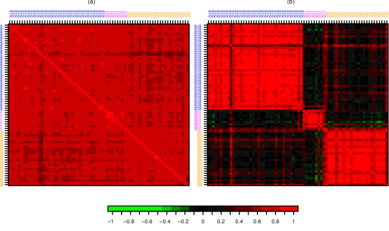
ijdenotes the expression level for gene j in mRNA sample i. Figure 1 displays images of the 72 72 correlation matrix between gene expression pro-
les for the 72 leukemia mRNA samples.
3.1.3 NC I 60. In this study, cDNA microarrays were used to examine the variation in gene expression among the 60 cell lines from the National Cancer Institute’s anticancer drug screen known as NC I 60 (Ross et al. 2000; http://genome- www.stanford.edu/nci60). The 60 cell lines are derived from tumors with different sites of origin: 7 breast, 6 central ner- vous system (CNS), 7 colon, 6 leukemia, 8 melanoma, 9 non–
small–cell lung carcinoma (NSCLC), 6 ovarian, 2 prostate, 8 renal, and 1 unknown (ADR-RES). Gene expression was stud- ied using microarrays with 9,703 spotted cDNA sequences. In each hybridization, uorescent cDNA targets were prepared from a cell line mRNA sample ( uorescent dye Cy5) and a reference mRNA sample obtained by pooling equal mixtures of mRNA from 12 of the cell lines ( uorescent dye Cy3). To investigate the reproducibility of the entire experimental pro- cedure (e.g., cell culture, mRNA isolation, labeling, hybridiza- tion, scanning), a leukemia (K562) cell line and a breast can- cer (MCF7) cell line were analyzed by three independent
ALLBALLB ALLBALLB ALLBALLB ALLBALLB ALLBALLB ALLBALLB ALLBALLB ALLBALLB ALLBALLB ALLBALLB ALLBALLB ALLBALLB ALLBALLB ALLBALLB ALLBALLB ALLBALLB ALLBALLB ALLBALLB ALLBALLB
ALLBALLBALLB ALLBALLBALLBALLBALLBALLBALLBALLBALLBALLBALLBALLBALLBALLBALLBALLBALLBALLBALLBALLBALLBALLBALLBALLBALLBALLBALLBALLBALLBALLBALLBALLBALLBALLBALLB
ALLTALLT ALLTALLT ALLTALLT ALLTALLT ALLT
ALLTALLTALLTALLTALLTALLTALLTALLTALLT
AMLAML AMLAML AMLAML AMLAML AMLAML AMLAML AMLAML AMLAML AMLAML AMLAML AMLAML AMLAML AML
AMLAMLAMLAMLAMLAMLAMLAMLAMLAMLAMLAMLAMLAMLAMLAMLAMLAMLAMLAMLAMLAMLAMLAMLAML
–1 –0.8 –0.6 –0.4 –0.2 0 0.2 0.4 0.6 0.8 1
ALLBALLB ALLBALLB ALLBALLB ALLBALLB ALLBALLB ALLBALLB ALLBALLB ALLBALLB ALLBALLB ALLBALLB ALLBALLB ALLBALLB ALLBALLB ALLBALLB ALLBALLB ALLBALLB ALLBALLB ALLBALLB ALLBALLB
ALLBALLBALLBALLBALLBALLBALLBALLBALLBALLBALLBALLBALLBALLBALLBALLB ALLBALLBALLBALLBALLBALLBALLBALLBALLBALLBALLBALLBALLBALLBALLBALLBALLBALLBALLBALLBALLBALLB
ALLTALLT ALLTALLT ALLTALLT ALLTALLT ALLT
ALLTALLTALLTALLTALLTALLTALLTALLTALLT
AMLAML AMLAML AMLAML AMLAML AMLAML AMLAML AMLAML AMLAML AMLAML AMLAML AMLAML AMLAML AML
AMLAMLAMLAML AMLAMLAMLAMLAMLAMLAMLAMLAMLAMLAMLAMLAMLAMLAMLAMLAMLAMLAMLAMLAML
(b) (a)
Figure 1. Leukemia Dataset (a) Correlation Matrix. Images of the correlation matrix for the 72 B-cell ALL, T-cell ALL, and AML samples based on expression pro’ les for p D 3,571 genes and (b) for the p D 40 genes with the largest BW ratio. Correlations of 0 are represented in black, increasingly positive correlations are represented with reds of increasing intensity, and increasingly negative correlations are represented with greens of increasing intensity. The color bar below the images may be used for calibration purposes. The mRNA samples are ordered by class,
’ rst B-cell ALL (blue), then T-cell ALL (magenta), and ’ nally AML (orange).
microarray experiments. Ross et al. screened out genes with missing data in more than two arrays. In addition, because of their small class size, the two prostate cell lines and the unknown cell line were excluded from our analysis. The data are summarized by a 61 51 244 matrix X D 4x
ij5, where x
ijdenotes the base 2 logarithm of the Cy5/Cy3 background- corrected uorescence intensity ratio for gene j in cell line i.
3.2 Imputation of Missing Data
For the lymphoma and NC I 60 datasets, each array contains a number of genes with uorescence intensity measurements that were agged by the experimenter and recorded as miss- ing data points. The mean percentage of missing data points per array is 6.6% for the lymphoma dataset and 3.3% for the NC I 60 dataset. Some of the discrimination methods discussed in Section 2 are able to handle missing data (e.g., CART), however, others require complete data (e.g., Fisher linear dis- criminant analysis). Missing data were imputed by a simple k nearest-neighbor algorithm, in which the neighbors are the genes and the distance between neighbors is based on the cor- relation between their gene expression levels across arrays.
For each gene with missing data, (a) compute its correlation
with all other p ƒ 1 genes, and (b) for each missing array,
identify the k nearest genes having data for this array and
impute the missing entry by the average of the corresponding
entries for the k neighbors. A value of k D 5 neighbors was
used for the lymphoma and NC I 60 datasets. For a detailed study of imputation methods in microarray experiments, the reader is referred to the recent work of Troyanskaya et al.
(2001), which suggests that a NN approach provides accurate and robust estimates of missing values.
3.3 Standardization
The gene expression data were standardized so that the observations (arrays) have mean 0 and variance 1 across vari- ables (genes). Standardizing the data in this fashion achieves a location and scale normalization of the different arrays.
In a study of normalization methods, we have found scale adjustment to be desirable in some cases to prevent the expres- sion levels in one particular array from dominating the aver- age expression levels across arrays (Yang et al. 2001). Fur- thermore, this standardization is consistent with the common practice in microarray experiments of using the correlation between the gene expression pro les of two mRNA samples to measure their similarity (Perou et al. 1999; Alizadeh et al.
2000; Ross et al. 2000).
3.4 Gene Selection
Many genes exhibit near-constant expression levels across tumor samples. We thus performed a preliminary selection of genes based on the ratio of their between-group to within- group sums of squares. For a gene j, this ratio is
BW4j5 D P
i
P
k
I4y
iD k54 Nx
kjƒ Nx
0j5
2P
i
P
k
I4y
iD k54x
ijƒ Nx
kj5
21
where Nx
0jand Nx
kjdenote the average expression level of gene j across all tumor samples and across samples belonging to class k only. The predictors were built using the p genes with the largest BW ratios. (Section 4 discusses selecting the value of p.)
Note that Golub et al. (1999) used a different method for standardizing the data and for selecting genes. For the sake of completeness, our comparison study includes the weighted gene voting scheme of Golub et al. with a
jcalculated using standard deviations instead of variances (Section 2.2) and with the data preprocessed as in Golub et al. (1999). We refer to the resulting predictor as “Golub,” and it is of interest to compare its performance with that of DLDA with data preprocessed as in Sections 3.3 and 3.4.
4. STUDY DESIGN
In the absence of genuine test sets, the different predictors are compared based on random divisions of each dataset into a learning set ¬ and a test set ´ . There are no widely accepted guidelines for choosing the relative sizes of these arti cial learning sets and test sets. A possible choice is to use leave- one-out cross-validation or to leave out a randomly selected 10% of the observations to use as a test set (Breiman 1996).
However, in our case, test sets containing only 10% of the data are not large enough to provide adequate discrimination between the classi ers. Because our main purpose is to com- pare classi ers, not to estimate generalization error, we choose
to sacri ce training data and increase test set size to one-third of the data (i.e., a 2:1 scheme).
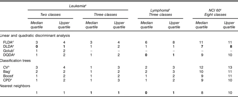
In the principal comparison, for each learning set/test set (LS/TS) run, the p genes with the largest BW ratio are selected using the learning set. For a comparison involving all predic- tors, FLDA sets an upper limit on the size of the gene set because of rank issues; the value of p for each dataset was chosen with these constraints in mind: p D 50 for the lym- phoma dataset, p D 40 for the leukemia dataset, and p D 30 for the NC I 60 dataset. Next, predictors are constructed using the LS and TS error rates are obtained by applying the predic- tors to the test set. Aggregated predictors (bagging and boost- ing) are built from B D 50 “pseudo” learning sets, and sev- eral values of the parameter d (d D 0051 011 0251 051 0751 1) were examined for CPD. This entire procedure is repeated N D 200 times. Each LS/TS run yields a test set error rate for each pre- dictor; the results are summarized by computing the median error rate for each predictor over the 200 runs (Table 1).
The effect of increasing (p D 200) or decreasing (p D 10) the number of genes is brie y examined. A “smarter” BW criterion is also applied to the lymphoma data. For p D 10 genes, this criterion consists of selecting the ve genes with the largest BW ratio (as before) and the ve genes with the largest BW ratio when the two largest classes (B-CLL and DLBCL) are pooled. Such a criterion should allow better dis- crimination of the smaller FL class.
5. RESULTS 5.1 Test Set Error
Table 1 displays the median and upper quartile of the num- ber of misclassi ed tumor samples for each classi er. For the leukemia dataset, the classi ers are compared based on their ability to distinguish between ALL and AML (two-class prob- lem), and between B-cell ALL, T-cell ALL, and AML (three- class problem). In general, the NN and DLDA predictors had the smallest error rates, whereas FLDA had the highest. With the exception of the NC I 60 dataset, the error rates seem fairly low given the small learning sets.
5.1.1 Nearest-Neighbor Classiers. The distance func-
tion used for the NN classi ers is one minus the correlation
between the gene expression pro les of two tumor mRNA
samples. The parameter k for the number of neighbors was
selected by cross-validation and was usually quite small for
each dataset: 1 or 2 for about half of the runs and gener-
ally less than 7. Although the small number of neighbors k
is an artifact of the small sample sizes, the results also sug-
gest that very good predictions can be obtained from the class
of the tumor sample most highly correlated to the sample
to be predicted. Indeed, for all three datasets, tumor samples
within the same class tended to have strongly and positively
correlated gene expression pro les (patches of red along the
diagonal of the correlation matrix in Figure 1). This pattern
is much more subtle for the correlation matrices based on
all genes and, as expected, the NN method bene tted greatly
from the initial selection of genes. The pattern is also stronger
for the lymphoma and leukemia data than for the NC I 60
data. (See web supplement http://www.stat.berkeley.edu/users/
terry/zarray/Html for gures for the NC I 60 and lymphoma data.)
5.1.2 Fisher Linear Discriminant Analysis. On the oppo- site end of the performance spectrum is FLDA. The most likely reason for the poor performance of FLDA is that with a limited number of tumor samples and a fairly large number of genes p, the matrices of between-group and within-group sums of squares and cross-products are quite unstable and pro- vide poor estimates of the corresponding population quantities.
The performance of FLDA dramatically improves and reaches error rates comparable to DLDA when the number of genes is decreased to p D 10, especially when the genes are selected according to the “smarter” BW criterion of Section 4 (see web supplement). Note also that FLDA is a “global” method, that is, it makes use of all of the data for each prediction, and as a result, some tumor samples may not be well represented by the discriminant variables. (There is only one discriminant variable for the two-class leukemia dataset and two discrimi- nant variables for the three-class lymphoma dataset.) In con- trast, NN methods are “local.”
5.1.3 Maximum Likelihood Discriminant Rules. The simple DLDA rule produced impressively low misclassi ca- tion rates compared with more sophisticated predictors, such as bagged classi cation trees. With the exception of the lym- phoma dataset, linear classi ers (i.e., DLDA), that assume a common covariance matrix for the different classes, yielded lower error rates than quadratic classi ers (i.e., DQDA), that allow for different class covariance matrices. Thus for the datasets considered here, gains in accuracy were obtained
Table 1. Test Set Error. Median and Upper Quartiles Over 200 LS/TS Runs, of the Number of Misclassi’ ed Tumor Samples for 9 Discrimination Methods Applied to 3 Datasets. For a Given Dataset, the Error Numbers for the Best Predictor are in Bold.
Leukemia
aLymphoma
bNCI 60
cTwo classes Three classes Three classes Eight classes
Median Upper Median Upper Median Upper Median Upper
quartile quartile quartile quartile quartile quartile quartile quartile
Linear and quadratic discriminant analysis
FLDA
d3 4 3 4 6 8 11 11
DLDA
e0 1 1 2 1 1 7 8
Golub
f1 2 – – – – – –
DQDA
g1 2 1 2 0 1 9 10
Classi’ cation trees
CV
h3 4 1 3 2 3 12 13
Bag
i2 2 1 2 2 3 10 11
Boost
j1 2 1 2 1 2 9 11
CPD
k1 2 1 3 1 2 9 10
Nearest neighbors
1 1 1 1 0 1 8 10
aLeukemia dataset from Golub et al. (1999), test set size nTSD 241p D 40 genes.
bLymphoma dataset from Alizadeh et al. (2000), test set size nTSD 271p D 50 genes.
cNCI 60 dataset from Ross et al. (2000), test set size nTSD 211 p D 30 genes.
dFLDA: Fisher linear discriminant analysis.
eDLDA: diagonal linear discriminant analysis.
fGolub: weighted gene voting scheme of Golub et al. (1999).
gDQDA: diagonal quadratic discriminant analysis.
hCV:single CART tree with pruning by 10-fold cross-validation.
iBag:BD 50 bagged exploratory trees.
jBoost: BD 50 boosted exploratory trees.
kCPD: BD 50 bagged exploratory trees with CPD, d D 075.
by ignoring correlations between genes. DLDA classi ers are sometimes called “naive Bayes” because they arise in a Bayesian setting, where the predicted tumor class is the one with maximum posterior probability pr4y D k—x5.
5.1.4 Weighted Gene Voting Scheme. For the binary class leukemia dataset, the performance of the variant of DLDA implemented by Golub et al. (1999) was also examined. This method performed similarly to boosting, CPD, and DQDA, but was inferior to NN and especially to DLDA, which had a median error rate of 0. Note that in contrast to the aggregated predictors in bagging and boosting, the “voting” is over vari- ables (here genes) rather than over classi ers. Furthermore, the gene voting scheme as de ned by Golub et al. (1999) is applicable to binary classes only; the closest generalization of it to multiple classes is the standard DLDA predictor, which was applied to the other datasets.
5.1.5 Classi cation Trees. CART-based predictors had
performance intermediate between the best classi ers (DLDA,
NN) and the worst classi er (FLDA). Aggregated tree pre-
dictors were generally more accurate than a single cross-
validated tree, with CPD and boosting performing better than
standard bagging. Several values of the parameter d, d D
0051 011 0251 051 075, were tried for the CPD method. For each
dataset, the best value turned out to be between 05 and 1, sug-
gesting that the performance of CPD was not very sensitive to
the parameter d controlling the degree of smoothing. A value
of d D 075 was used in Table 1.
5.2 Individual Misclassi’ cation Rates
Prediction votes for aggregated predictors may be used to summarize the strength of individual predictions and possibly reveal errors in diagnosis. For the two-class leukemia dataset, Figure 2 displays plots of the proportions of correct classi ca- tions and three number summaries (median, lower, and upper quartiles) of the boosting prediction votes (PVs) and Golub et al. (1999) prediction strengths (PSs) for each tumor sam- ple over the 200 LS/TS runs. The qualitative correspondence between PVs and proportions of correct classi cations sug- gests that PVs are good indicators of a predictor’s ability to correctly classify a particular tumor sample. The Golub PSs seem to be highly variable and conservative in comparison to the proportions of correct predictions, perhaps because the
“voting” is over genes rather than over predictors as in PVs.
Furthermore, the summands in the PSs involve expression lev- els for individual observations, whereas the summands in PVs involve weights, which are computed using the entire learning set. Similar results were observed for bagging PVs and other datasets (see the web supplement).
5.2.1 Lymphoma. For the lymphoma dataset, two tumor samples tended to be dif cult to classify and had small pre- diction votes (see the web supplement for more details). The
rst observation (index 1, CLL-70; lymph node) is a B-CLL case, but the mRNA sample was prepared from a lymph node biopsy specimen rather than from peripheral blood cells as for other B-CLL cases. This tumor sample tended to be clas- si ed as an FL case, perhaps re ecting tissue sampling. The other observation (index 39, DLCL-0042) is believed to be a DLBCL case and tended to be classi ed as an FL case. The FL cases were generally harder to classify and had smaller prediction votes than tumor samples from other classes; this
Observations 0
1
PV quartiles
0 1
% correct predictions0 10 20 30 40 50 60 70
(a) Boosting PV
Observations 0
1
PS quartiles