阿根廷魷魚之食性分析與人造物攝入

(1)

國立臺灣大學生命科學院漁業科學研究所碩士論文

Institute of Fisheries Science College of Life Science National Taiwan University

Master Thesis

阿根廷魷魚之食性分析與人造物攝入

Feeding habits of the Argentine short-finned squid

Illex argentinus, including artifact ingestion

張思維 Ssu-Wei Chang

指導教授：柯佳吟博士 Advisor: Chia-Ying Ko, Ph.D.

中華民國 109 年 7 月 July 2020

(2)

口試委員會審定書

(3)

致謝

我要先感謝我的指導教授柯佳吟老師，在研究的過程中給予我許多建議與想法，讓我得以在錯誤中學習並且能完整的完成這個研究。我也要感謝擔任我口試委員的丘臺生老師、戴昌鳳老師與陳志炘老師，給予我論文內容詳盡的改善建議。

在我進行的各項實驗中，我要感謝在同步輻射中心提供我使用FTIR 儀器與技

術指導的李耀昌博士與佩瑜學姊。在研究中魚類耳石的鑑定，我要感謝林千翔博士

百忙之中的協助。我也要感謝借我使用儀器與藥品的周宏農老師、睿哲學長與beth

學姊。在研究摸索階段，我要感謝提供我儀器與技術指導的陳玟伶老師與嘉聲。

在 304 研究室中朝日相處的各位，我要謝謝瑞谷學長不厭其煩的教導與協助

我解剖魷魚；謝謝旻祐與馬霽帶給我研究與人生的方向；謝謝Lisa 學姊、Daniel 學

長與 Mason 為我帶來一股活水；謝謝光瑢姊與阿姨在我實驗時的幫忙；謝謝魷魚

大哥璁翰不管在日常還是研究中的關懷備至；謝謝Erica 在我論文與投影片上英文

的幫忙；謝謝穎禎在我後續分析時給我很大的幫助；謝謝子謙在論文與健身上的幫助；謝謝靖雲常給我實用的建議；謝謝孝謙對我口試投影片的建議；謝謝晴芳在剛進研究室的幫忙；謝謝芝瑋在生統後期時的幫忙；謝謝士瀚對研究室大小事的付出；

謝謝偉哲帶給我生活中的樂趣；謝謝裕庭偶爾的探訪與幫忙；謝謝承庭、葆仁、昀翎在研究室的幫忙。我也要謝謝漁科所、海研所與其他我的同學們，謝謝你們在日常與研究上的幫忙。

此外，我要感謝我的家人讓我在無慮的情況下完成我碩班的學業，有你們作為強大的後盾我感到很安心。

最後，在我實驗過程中犧牲的各種生物，感謝祢們的付出讓我得以順利完成我的研究。

張思維謹誌於國立臺灣大學漁業科學研究所中華民國一零九年八月七日

(4)

中文摘要

頭足類（Cephalopods）中在生態學與漁業皆扮演重要角色，為全球重要漁獲

資源之一，年產量約占總漁獲量的 4%。頭足類中的魷類（Squids）具有多樣化的

食性以及豐富的族群量，在食物網中做為高級消費者提供不同營養階層間高度交互作用及能量流動。過去研究已顯示在氣候變遷衝擊下，魷類的主要食物來源如磷蝦也因海冰溶化導致棲地改變而降低生物量。然而，對於快速生長過程中須攝食大量食物的魷類而言，目前尚未有研究探討魷類是否會因上述原因影響其食性，以及

近年的海洋塑膠汙染對其攝食的影響。在本研究中，利用2018 及 2019 年 2 月到 4

月在西南大西洋所採集之300 尾阿根廷魷（Illex argentinus），解剖個體胃內容物，

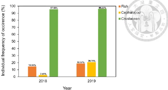
進行食性分析與人造物檢測。由食性分析結果顯示，在2018 年有 97.60%的阿根廷

魷個體胃內容物中含有甲殼類、14.90%含有魚類以及 2.40%含有頭足類；在 2019

年有 96.23%的阿根廷魷魚個體胃內容物中含有甲殼類、18.87%含有魚類以及

20.75%含有頭足類，可以發現阿根廷魷魚在 2019 年攝食頭足類的比例明顯較高，

攝食甲殼類的比例明顯較低。由人造物檢測結果顯示，阿根廷魷魚個體的人造物攝

取比例在2018 年為 17.92%、在 2019 年為 28.33%，但阿根廷魷個體平均攝取人造

物數皆小於0.5 個，並且由 FTIR 分析結果顯示大部分人造物並非塑膠但可能為似

衣料纖維的聚醣材質。整體而言，阿根廷魷魚的食性雖因年度有部分差異，但攝食內容整體比例仍與前人研究相近，顯示其食性應未隨氣候變遷改變，而人造物檢測結果也顯示西南大西洋海域僅輕微污染，可提供國民對於此類食品安全的參考。

關鍵字：頭足類、魷魚、阿根廷魷、食性、氣候變遷、人造物汙染

(5)

Abstract

Cephalopods play an important role in ecology and fishery. The variation in the diet of large squid population promote high interaction of individuals between different trophic levels in the marine ecosystem. As a consequence of global climate change, previous research has indicated that alteration of environment impacts the availability of the prey. Due to marine pollution, the squids are under the risk of artifact ingestion.

However, no clear understanding about the effect of climate change and marine pollution on squid diet selection. This study examined 300 stomachs from Illex argentinus. The sample were collected through commercial catches across the Southwest Atlantic from February to April of 2018 and 2019. In the result, the percentage of frequency of occurrence (FO%) of squid diet in 2018 comprised of 14.90% fish, 2.40% cephalopod and 97.60% crustacean taken from 208 stomachs. Meanwhile, a relatively higher FO%

for squid diet in 2019 was observed comprising of 18.87% fish, 20.75% cephalopod and 96.23% crustacean examined from 53 stomachs. Also, the Fourier-Transform Infrared Spectroscopy (FTIR) showed that artifacts examined were composed of plastic and non- plastic materials. Subsequently, FO% of artifact ingestion was higher in 2019 (28.33%) than in 2018 (17.92%), thus mean number of artifact ingestion from two years were less than 0.5. The results indicate that the main diet of Illex argentinus is crustacean. Also, climate change has no direct impact to the squid diet. The results of artifact detection showed that the Southwest Atlantic is less polluted. Thus, it is suggested to continue a monitoring study of squids in this area, particularly on food safety and diet to well manage the biodiversity and squid biology.

Keywords: Cephalopod, Squid, Illex argentinus, Diet, Climate change, Artifact pollution

(6)

List of figures

Fig. 1 The sampling locations of Illex argentinus in the Southwest Atlantic in 2018 and 2019... 38 Fig. 2 The composition of mantle length of Illex argentinus in 2018 and 2019 ... 39 Fig. 3 The composition of mantle length of Illex argentinus in different months of 2018 and 2019... 40 Fig. 4 The correlation between latitude of sampling location and mantle length of Illex argentinus in 2018 and 2019 ... 41 Fig. 5 The percentage of stomach fullness index of Illex argentinus in 2018 and 2019

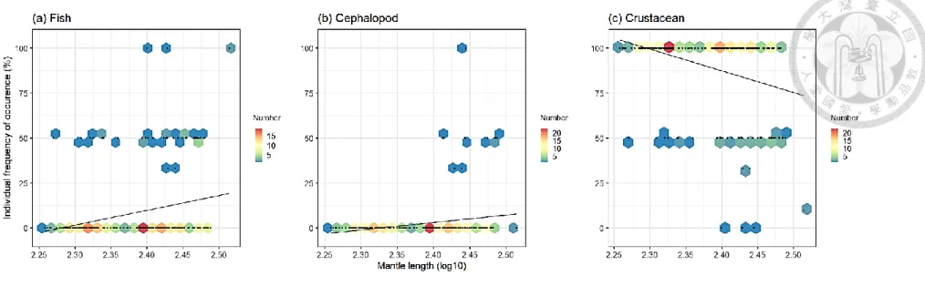
... 42 Fig. 6 The overall percentage of frequency of occurrence and number of the three main diets of Illex argentinus in 2018 and 2019 ... 43 Fig. 7 The individual percentage of frequency of occurrence of the three main diets of Illex argentinus in 2018 and 2019 ... 44 Fig. 8 The percentage of 50 mm mantle length intervals of Illex argentinus with different stomach fullness index in 2018 and 2019 ... 45 Fig. 9 The individual percentage of frequency of occurrence in three main diets in 50 mm mantle length intervals of Illex argentinus in 2018 and 2019 ... 46 Fig. 10 Hexbin plot of individual percentage of frequency of occurrence in relation to mantle length (logarithm base 10 transformation) in three main diets of Illex argentinus in 2018 ... 47 Fig. 11 Hexbin plot of individual percentage of frequency of occurrence in relation to mantle length (logarithm base 10 transformation) in three main diets of

(9)

Illex argentinus in 2019 ... 48 Fig. 12 The percentage of stomach fullness index of Illex argentinus with artifact ingestion in 2018 and 2019 ... 49 Fig. 13 The individual percentage of frequency of occurrence of artifacts in 50 mm mantle length intervals of Illex argentinus in 2018 and 2019 ... 50 Fig. 14 Hexbin plot of individual percentage of frequency of occurrence of artifacts in relation to mantle length (logarithm base 10 transformation) of Illex argentinus ... 51 Fig. 15 Monthly variations in sea surface temperature in the distribution range of Illex argentinus in 2018 and 2019 ... 52 Fig. 16 Monthly variations in Chlorophyll a concentration in the distribution range of Illex argentinus in 2018 and 2019 ... 53

(10)

List of tables

Table 1 Sampling of Illex argentinus in different sampling locations in 2018 and 2019

... 54

Table 2 The summary of preys of Illex argentinus in 2018 and 2019 ... 55

Table 3 The diet of Illex argentinus with artifact ingestion in 2018 and 2019 ... 56

Table 4 The summary of artifacts in Illex argentinus in 2018 and 2019 ... 57

Table 5 The correlation between mantle length of Illex argentinus and Sea surface temperature ... 58

Table 6 The correlation between mantle length of Illex argentinus and Chlorophyll a concentration... 59

(11)

Chapter 1 Introduction

1.1 The impact of climate and environmental changes

Serious ecological alterations have appeared in global marine environment at fast rate (Poloczanska et al., 2013). Long-term climate change and short-term changes in the environment affect the resource availability of marine organisms. Diet shift of the marine organisms is the result of the changes in food availability. Long-term changes in primary production have influenced in the marine food web due to bottom-up controls (Frederiksen et al., 2006; Hays et al., 2005). Climate change at long time scales cause alterations in marine habitat distribution and predator-prey interaction (Green & Côté, 2014; Hazen et al., 2013). Distribution of krill in the Southwest Atlantic has changed due to the loss of sea ice under long-term climate change (Atkinson et al., 2019). Population of krill predators such as penguins declined because of food shortage (Klein et al., 2018).

Short-term changes in environmental conditions alter prey availability and preference of predators (Scharf et al., 2000; White, 2008). Top predators such as seabirds often rely on limit species of prey (Cury et al., 2000). If prey availability changes due to environment alteration, it may have consequences on the foraging behavior or animal diet composition.

Therefore, determining the relationship between diet dynamics of marine organisms and global climate can help to better understand the impacts of environmental changes to marine animals.

1.2 Ecological characteristics of squids

Squids are insatiable predators feeding opportunistically on variable diets (Rodhouse

(12)

& Nigmatullin, 1996). They are important prey of top predators (Clarke, 1986; Klages, 1996; Smale, 1996). These characteristics make them become the key role between different trophic levels in the marine ecosystem (Piatkowski et al., 2001). Furthermore, resulting from overexploitation of fish stocks and changing marine environment, their population may increase by replacing trophic niche of fishes (Caddy & Rodhouse, 1998;

Doubleday et al., 2016; Hoving et al., 2013). These changes in marine biodiversity due to overexploitation favors the squids to having more essential roles in the marine food web.

Because of the short lifespan of squids, they are susceptible to environmental change (Rodhouse & Nigmatullin, 1996). Previous studies have indicated that climate change may increase the distribution of squids and influence the relationship of species in other ecosystems (Golikov et al., 2013; Zeidberg & Robison, 2007). However, there is limit knowledge on the diet of squids in the area with environmental alteration (Collins &

Rodhouse, 2006).

1.3 Diets of Illex argentinus

Cephalopods contribute significantly to the ecology and fishery due to their large population (Doubleday et al., 2016). They are important resources in the global fishery which account for approximately 4% of the total catch and 5% of total value. Among cephalopods, Illex argentinus are major resources in global cephalopod fishery as well as account for nearly 10% in total catch of cephalopods (FAO, 2019). Illex argentinus have short life span of about one year and they die after spawning (Rodhouse & Hatfield, 1990).

To achieve high growth rates for fast-growing, Illex argentinus require great abundance of food (Haimovici et al., 1998). Therefore, they undergo horizontal and vertical

(13)

migrations in the daytime and early night for prey availability (Ivanovic & Brunetti, 1994;

Santos & Haimovici, 1997).

According to previous studies, Illex argentinus have dissimilar diet composition in different latitude interval, they consume more crustaceans in the southern distribution (Ivanovic & Brunetti, 1994). Moreover, diet analysis in various years represent Illex argentinus have fluctuating diets (Ivanovic & Brunetti, 1994; Mount et al., 2001; Rosas- Luis et al., 2014). Antarctic, a close region of squid distribution, has been observed as a significant area impacted by climate change in the 21st century (Jansen et al., 2007). The changes in the sea surface temperature (SST) and chlorophyll a concentration (Chl-a) in sea area caused a reduction in krill population which later on replaced by other crustaceans (Murphy et al., 2007; Atkinson et al., 2012). Squids have different diets due to their size in each life stage and food abundance in their habitats. Therefore, squid may have diet shift when the population of crustacean also changed (Rodhouse & Nigmatullin, 1996; Rodhouse, 2013).

1.4 Recent concerns of marine artifact pollution

Marine artifact pollution and ingestion by marine organisms are of major concern recently in studying marine environment and ecology. Plastic productions are growing consistently due to great demand (PlasticsEurope, 2018). Some artifacts are made of plastics that break down to microplastics. This mostly accumulate in marine ecosystems causing an environmental pollution (Van Sebille et al., 2015). Ingestion of microplastic causes diverse effect on marine organisms (Avio et al., 2015; Cole et al., 2015). Some artifacts are manufactured from natural materials such as cotton, silk and wool; however, the processing of these artifacts contained carcinogenic chemicals which lead to a

(14)

potential health risk (Acuner & Dilek, 2004; Khan & Malik, 2013). Squids consume great amount of food throughout their ontogeny. The inclusion of artifacts, especially plastics, in the squid’s food can become a serious problem owing to the bioaccumulation in the food web as well as the food safety issues. Nevertheless, there are lack of studies about the risk of artifact ingestion in squids. Only few studies about diet analysis and food safety of commercial cephalopods include artifact ingestion (Rosas-Luis, 2016; Abidli et al., 2019). In the distribution of Illex argentinus, only some studies are about artifact ingestion in top predators. 14.5% of the opah fish distributed near the Falkland Islands contained artifacts in their stomachs and 20% of the gentoo penguin distributed in the Antartic region contain artifacts in their scats (Jackson et al., 2000; Bessa et al., 2019).

1.5 Objectives

Due to lack of information about diet shift by environmental alteration and artifact ingestion of the squids, in this study we analyzed the diet of Illex argentinus. We compare squid’s diet in 2018 and 2019 with previous studies. Moreover, we examined the relationship between the environment and biological information of Illex argentinus, including body size, stomach fullness and diet. Finally, we examined the level of artifact ingestion by Illex argentinus and compare it with the results of diet analysis to find out if there are any relations.

(15)

Chapter 2 Materials and Methods

2.1 Study area and stomach sampling

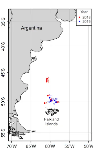
Illex argentinus were collected from commercial catches of Taiwanese jigging vessels across the northern open sea of Argentina from February to April 2018 and 2019 (Fig. 1). The squids were collected once every two weeks whenever the jigging location was changed. The numbers of each collection followed the size of frozen iron boxes on the vessels. In general, two boxes were filled up with squids. During dissection, dorsal mantle length (ML), body weight, sex and maturity stage (Lipinski & Underhill, 1995) were recorded for all the samples. Individual stomachs were extracted and frozen at - 20°C. In this study, we selected only female squids in each location due to low catch in male squids.

2.2 Stomach content analysis

Stomachs were weighed after defrosting and excising the caecum. Caecum of squid contained nutrient fluid digesting from solid particles in the stomach (Bidder, 1950).

Caecum was excised before examining due to the difficulty in content examination of the mucous lining in the stomach. Hence, the stomach was first examined for diet analysis.

Then, the rest of stomach contents were dissolved for artifact detection after the preservation of the identified prey items

2.2.1 Diet analysis

A visual stomach fullness index (SFI) was estimated: 0 = empty; 1 = scarce; 2 = few;

3 = half full; 4 = full; 5 = full to distended (Breiby, 1985). Stomachs were opened and

(16)

contents were rinsed over 200 and 330 µm mesh sieves. The identification and quantification of prey contents in the stomach were done using a binocular dissecting microscope. Prey items were identified to the lowest possible taxon. Fish remains, such as sagittal otoliths were identified based on Lombarte et al. (2006). Cephalopod remains, such as beaks were identified based on identification keys of Clarke (1986) and photographs in Xavier & Cherel (2009). Crustacean remains, such as exoskeletons were identified following the descriptions on Boschi et al. (1992) and Chapman (2007).

Quantification of prey items was executed by calculating overall and individual frequency of occurrence (FO) in a sample and number (N) (Mouat et al., 2001; Markaida & Sosa- Nishizaki, 2003; Markaida et al., 2008).

Overall frequency of occurrence (FO%) = Number of stomachs with certain prey type Total observation of all prey types

Individual frequency of occurrence (FO%) = Number of stomachs with certain prey type Total number of stomachs with prey

Overall number (N%) = Number of certain prey type Total number of all prey types

Individual mean number (N) = Number of certain prey type Total number of stomachs with prey

The amount of fish prey was counted by the maximum number of otoliths or lens.

Cephalopod prey was enumerated by the maximum number of statoliths, lens or beaks.

Although tentacle fragments appeared in some stomachs, we removed them from the numbers of cephalopod prey since squid cannibalizes tentacles of the others when gathering on the board. Due to manducation of squid on their preys, number of crustacean was hard to assess. As a result, a conventional estimation was used to record crustacean prey as presence (n = 1), or absence (n = 0) (Portner et al., 2019). Overall and individual

(17)

FO and N were compared with each year and ML.

2.2.2 Artifact detection

The remaining stomach contents were dissolved by 10% KOH in 60°C incubation for 48 h (Jamieson et al., 2019; Lusher et al., 2017). KOH was added as three times greater volume of the stomach contents (Foekema et al., 2013) to digest the biological particles in the contents with artifacts remaining (Dehaut et al., 2016; Kühn et al., 2017). Water bath was used to incubate the dissolving contents. Contents were shaken for 30 seconds to promote digestion every day. Dissolved contents were filtered through Whatman Grade 541 filter paper and moved to petri dish for examination under a binocular dissecting microscope (Jamieson et al., 2019). Used filter papers were inspected visually for the artifacts and kept in tin foil for further analysis. If artifacts were found, they were photographed and scaled by software “ImageJ” (v.1.52a; https://imagej.nih.gov/ij/).

To prevent contamination, laboratory coats and nitrile gloves were worn when processing experiment. Every equipment and container were rinsed with acetone or 70%

ethanol before use. During each experimental procedure mentioned above, two clean petri dishes with distilled water were placed on left and right side of the processing area to collect possible contamination (Baalkhuyur et al., 2018). After finishing each procedure, petri dishes were examined and the amounts of contamination were recorded.

The characterization of artifacts found in filter papers were analyzed by Fourier- transform infrared spectrometer (FTIR; INVENIO R, Bruker, Ettlingen, Germany) at TLS 14A1 of National Synchrotron Radiation Research Center in Taiwan. An IR microscope (Hyperion 3000, Bruker, Ettlingen, Germany) is integrated with the spectrometer for FTIR imaging and a single element Mercury-Cadmium-Telluride (MCT) cooled by liquid

(18)

nitrogen is also equipped. Spectral range of the apparatus is 4000-650 cm^-1 at resolution of 4 cm^-1 in 64 scans. The spectral results of the artifacts were compared with spectra library of the software “OPUS” (v.8.1) and confirmed by the inspection of peaks matching.

Identified artifacts were then calculated with the total numbers of stomach for individual N and FO and compared with each year and ML. Moreover, individuals with artifact ingestion compared with their SFI and diet composition.

2.3 Environmental data

Sea surface temperature (SST) and Chlorophyll a concentration (Chl-a) were included to measure environmental conditions in the main distribution area (34°S – 55°S and 50°W – 70°N) of Illex argentinus (Ivanovic & Brunetti, 1994). Due to the duration for more than one to two days of food remained in the stomachs (Bidder, 1966), daily data were collected and calculated the mean value of 0 day, -1 day, -2 days, -3 days, -5 days and -7 days of sampling. The variation of environmental data in sampling period of two years would later compare with diet and artifact consumption. SST data at 0.25 × 0.25 spatial resolution was obtained from the National Oceanic and Atmospheric Administration (NOAA) (https://www.ncei.noaa.gov/). Chl-a data at 4 km × 4 km spatial resolution was obtained from the Copernicus Marine Environment Monitoring Service (CMEMS) (http://marine.copernicus.eu/).

2.4 Statistical analysis

A nonparametric Kruskal-Wallis test with Dunn's multiple comparisons post hoc test was used to determine the differences in ML between months and years. Linear

(19)

regressions were used to analyze the relationship between the diet/artifact consumption and mantle length in different months in each year. The Pearson correlation coefficient was used to evaluate relationship between different duration of mean environmental data and ML in two years. All analyses were performed in R V4.0.1 (R Core Team, 2020).

(20)

Chapter 3 Results

3.1 Sample description

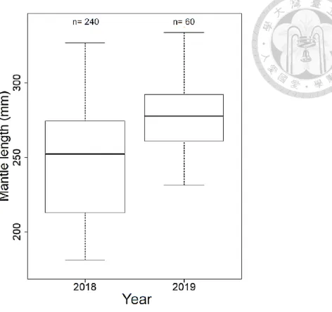
We selected 30 individuals per sampling station in 2018 and 240 individuals in total, whereas there were 60 individuals in total in 2019 (Table 1). A total of 300 squids were prepared for further analysis. Squids’ ML range were 181.2 mm to 333.8 mm. The minimum ML was 181.2 mm in 2018, while the maximum ML was 333.8 mm in 2019.

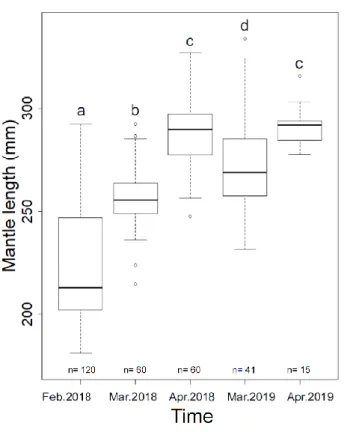
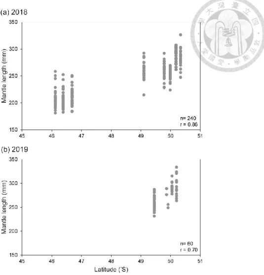
Mean ML in 2019 was about 30 mm higher than that in 2018. Standard deviation (SD) of ML in 2018 was 34.94, a much higher than 22.02 in 2019. This indicated that ML in 2018 was more dispersed. The SD range in 2018 was 10-18 while 4-21 in 2019. The location with less individual samples in 2019 tended to have lower SD. ML between two years had significant difference (p < 0.01). The ML in 2019 was larger than the ML in 2018 (Fig. 2). Comparing the ML in different months from the two years (Fig. 3), the ML in March from two years was significantly different (p < 0.01). Take note that the ML in March 2019 was larger than the ML in march 2018. Meanwhile, ML in April from two years had no difference (p = 0.33). ML from February to April in 2018 and from March to April in 2019 had significant difference. ML in 2018 and 2019 increased along with months. A positive correlation between latitude of sampling location and ML of Illex argentinus in 2018 and 2019 indicate that ML represented the growth and the trend of migration (Fig. 4). Due to the difference between months and years as well as the positive relationship with latitude, ML was used as comparing benchmark for further analysis.

(21)

3.2 Diet analysis

3.2.1 Stomach fullness

The SFI in 2018 had higher percentage (SFI = 3, 4 and 5), which showed most individual stomachs were more than half full (Fig. 5). The SFI 0 in 2019 was less than other level. This indicated that most individuals had food remained in their stomachs.

Empty stomachs (SFI = 0) were removed and would not be used in diet analysis, including n = 32 in 2018 and n = 7 in 2019.

3.2.2 Diet composition

The identified fragments composed of 147 fish, 28 cephalopod and 9353 crustacean observed in 208 stomachs in 2018. Meanwhile, 88 fish, 37 cephalopod and 2602 crustacean fragments observed from 53 stomachs in 2019. The diet composition of Illex argentinus involved fishes, cephalopods and crustaceans in two years (Table 2).

Crustaceans were main diet of squid in this study. The diets in 2018 were diverse than diets in 2019. Squids consumed 5 different fish species in 2018 but only 2 species in 2019.

Unique species of fish in 2018 were the genus Rhynchohyalus, Notophycis marginata and Micromesistius australis, while the genus Dolichopteryx and Gymnoscopelus nicholsi observed in both years. Distinct cephalopod species consumed by squid in 2018 was Loligo gahi. Illex argentinus and Histioteuthis atlantica were found in stomachs of squid of two years and showed that squid in this study had cannibalism. Diet species of crustaceans remained identical in both years, including the order Amphipoda, Decapoda and Euphausiacea.

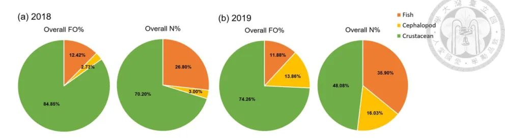
In comparison with the overall FO% and N% of three main diets in 2018 and 2019, fishes had similar overall FO% in stomachs in two years (12.42% and 11.88%) but overall

(22)

N% was higher similar by 9% in 2019 (Table 2). These denoted that overall occurrence of fishes in stomachs were similar, yet overall squid consumed larger numbers of fishes in 2019 (Fig. 6). Overall FO% and N% of cephalopods in 2019 were higher than overall percentage of cephalopods in 2018 by more than 10%. Overall FO% of crustacean consumption in 2019 was 10.59% less than percentage in 2018, while overall N% in 2019 was 22.12% less than percentage in 2018. Comparing individual FO% in two years, percentage of fishes in 2019 was larger than percentage in 2018 (Fig. 7). Nevertheless, cephalopods had apparently higher individual FO% in 2019. The mean number of individual of each diet in 2019 was greater than that in 2018 (Table 2). The value in the diet of fishes and cephalopods in 2019 was approximately 0.5 larger than value in 2018 as well as individual mean N of crustaceans was 0.07 higher in 2019.

3.2.3 The relationship between diet and individual size

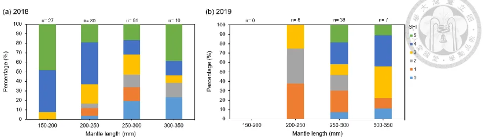
The comparison between SFI and ML in two years revealed that each SFI was distributed in all ML intervals, but SFI was different concentrating in each interval (Fig.

8). In 2018, individuals in 150-200 mm and 200-250 mm had higher percentage in SFI 3- 5. In 2019, individuals in 200-250 mm had higher percentage in SFI 1-3.

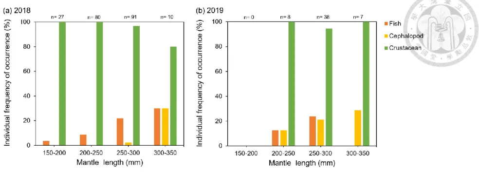
The relationship between ML and individual FO% was shown (Fig. 9). The squid with larger ML tended to have higher cephalopod consumption. Individual FO% of fishes and cephalopods in two years increased as ML became larger. In 2018, cephalopod mostly appeared in the stomachs of individual in 300-350 mm. Crustaceans had lower individual FO% from 250-300 mm to 300-350 mm. In 2019, squid in 300-350 mm did not consume fishes. Individual FO% of crustacean was similar in each ML interval. Evidently, there was higher individual FO% of cephalopod in 200-300 mm in 2019.

(23)

In 2018, fishes and cephalopods were similarly concentrated in individual FO% 0, indicating most squids did not consume these species (Fig. 10). Individual FO% of crustaceans concentrated in 100 at the left side of ML, indicating most smaller individuals only consume crustaceans. There was similar distribution at individual FO% 50 in the diets of fish and crustacean, therefore the represented diets of fish and crustacean were included in some individuals. Large squid consumed more cephalopod since the FO%

value above 0 in cephalopods located at the right side of ML. Individual FO% of fishes and cephalopods increased along with individual ML. In contrast, the individual FO% of crustaceans decreased while ML increased (Fig. 10). In 2019, other than the similar concentration of individual FO% 0 in fishes and cephalopods as well as 100 in crustaceans, the distribution was more scattered than the one in 2018 (Fig. 11). There was more distribution at the individual FO% 30 in three main diets, which indicated more individuals were consumed as diets including fish, cephalopod and crustacean. In addition, individual FO% 50 observed more in the diets of cephalopod and crustacean.

Regression lines of cephalopod and crustacean were nearly horizontal and showed no trend between FO and ML. The regression line of fish had slightly upward trend, which indicated individual FO slightly rose as ML increased. The relationship between cephalopod and crustacean showed no trend between FO and ML (Fig. 11). While, fish weak positive relationship with ML.

3.3 Artifact detection 3.3.1 Artifact classification

A total of 76 artifacts were found in stomachs of 300 individuals from 2018 and 2019

(24)

samples. Three types of artifact were observed in this study, including 69 fibers, 3 films and 4 fragments. Various colors in artifacts were detected, which contained blue in 61 artifacts, red in 9 artifacts, green in 2 artifacts and Black (Grey) in 4 artifacts. The most abundant artifacts among all was blue fiber.

3.3.2 Stomach fullness and diet of artifact consuming individuals

Most individuals within the two years of study had only consumed crustaceans while some individuals had no food remained in their stomachs (Table 3). The proportional distribution of SFI among artifact-consuming individuals was distinctive in two years. In 2018, individuals with SFI 4 and 5 had higher artifact ingestion. Comparing with the percentage in 2018, individuals in 2019 had greater artifact ingestion at SFI 1 and 2.

Artifact-consuming individuals in 2018 had similar SFI with overall individuals in 2018 (Fig. 12). In 2019, the percentage of SFI 0 in artifact-consuming individuals was two times as large as percentage in overall individuals, while percentage of SFI 4 in 2019 was nearly 3 times less.

3.3.3 Artifact composition

A total of 6 artifacts were identified as plastics including nylon 66 and polyethylene terephthalate (PET) (Table 4). Most artifacts were unidentified, only 13.33% in overall FO% in 2018 was plastic. Squid had greater artifact ingestion in 2019 as individual FO%

and individual mean N of artifacts were higher than that in 2018. Nevertheless, individual mean N in two years was less than 0.5 which indicated there were small amount of artifact ingestion in squid in this study. In addition, mean contamination on petri dishes was approximately 0.1 which were non-artifacts and were not be used in this study. Thus, the

(25)

airborne contamination was not a serious problem.

3.3.4 The relationship between artifact ingestion and individual size

Larger squid in two years had greater individual FO%, though the percentage was different in some ML intervals between the two years (Fig. 13). In 2018, the Individuals with 150-200 mm and 200-250 mm ML had similar FO%. Also, the individual FO%

increased as ML increased from 200-250 mm, 250-300 mm to 300-350 mm. In 2019, individual FO% were similar in 200-250 mm and 250-300 mm, though the percentage grew with apparently increasing ML from 250-300 mm to 300-350 mm. FO% of artifacts in two years were concentrated in 0 and represented most individuals had no artifact ingestion (Fig. 14). In addition, the individual FO% and larger ML showed a positive relationship. More evident trend in 2019 was shown due to the steeper slope of regression line.

(26)

Chapter 4 Discussion

4.1 Diet analysis

Crystalline lens is necessary for identifying the diet in squid. However, cephalopod and fish have similar appearance of lens. In this study, we differentiated the lens in the stomachs by soft stabbing with tweezers. If the lens could easily separate into two parts, it would be the lens of cephalopod (West et al., 1995). Fish lens is usually spherical and cannot be separated. Previous studies about diet of cephalopod rarely used lens to identify cephalopod. Therefore, adding lens as the key for identifying cephalopod would make the diet of cephalopod more clearly. The statoliths of cephalopod were seldom found in the stomach directly, while they were often found in a translucent tissue. It seems like that the statoliths are more susceptible by gastric acid than otoliths of fish and correspond with the negative effect of ocean acidification in the development of statolith (Kaplan et al., 2013). Conventional estimation would lead to smaller amount of crustacean counting.

Nevertheless, putting all fragments of crustacean into counting would have greater error as the fragments of three main diets in two years were 235 pieces of fish, 65 pieces of fish and 11955 pieces of crustaceans.

In this study, the overall FO% of fish in two years in this study were 10% higher than the percentage in the previous study in 1992 (Ivanovic & Brunetti, 1994). In contrast, the overall FO% of cephalopod in 1992 was 10% greater than the value in 2018 and the percentage of crustacean was 10% higher than the value in 2019. The difference between three main diets would indicate there was more predation of fish by the squid in this area in recent years, though the predation of cephalopod and crustacean was fluctuated. The relationship of ML and diets in 1992 was only apparent in the diet of crustacean. The

(27)

overall FO% of amphipod became higher as the ML increased but the percentage of euphausiid decreased. However, the percentage of amphipod decreased along with ML increased in two years. The relationship between overall FO% and ML in 1992 was similar to the trend in 2019, while it was contrary to the trend in 2018. The euphausiid seemed to have fluctuating population in these years, hence amphipod would be less important in the diet of larger squid. Individual FO% of fish and crustacean had lower value in the previous study in 1998 (Mouat et al., 2001), while the percentage of cephalopod was approximately 9 times larger than the value in 2018 in this study. Lower value of fish and crustacean in 1998 might result from lack of food as percentage of cannibalism reached up to 12.24% in 1998. The SFI distribution in the previous study in 2012 was similar to the distribution in 2018, which represented most stomachs of both years were full (Rosas-Luis et al., 2014). The individual FO% in the study in 2012 had 3 to 4 times larger value in fish and about 7 times less value in crustaceans. The possible reason of difference in FO% would be the more southern sampling location in 2012 which might lead to different diet composition of squid.

Due to lower catch in each location, the sampling size in 2019 was 3 times less than the size in 2018. Aside from the sampling size in two years, environmental data could provide possible explanation about variation between diet composition of the two years.

Abundance of cephalopod population was influenced by the SST in their habitat and higher SST led to greater abundance of cephalopod population (Waluda & Pierce, 1998;

Doubleday et al., 2016). There was lower SST in 2019 from the end of February to the middle of March (Fig. 15), which resulted in smaller population of squid. Less competition in smaller population lets squid in 2019 become larger and can consume species in greater size such as fish and cephalopod. Lower chl-a in sampling period of

(28)

2019 (Fig. 16) may cause lower primary productivity, which leads to reducing population of planktonic crustacean (Legendre & Rassoulzadegan, 1995). Planktonic crustacean such as amphipod is the necessary diet of Illex argentinus. From lower diet species composition and dispersed SFI, there may have less food abundance in sampling area of 2019. This may also be explained by the related day of environmental data. In 2018, three days before sampling were the most related to ML in 2018 which may indicate squids in 2018 consume more foods as well as the foods remained in their stomach for 2 - 3 days.

However, the most related day in 2019 was the day of sampling which indicated that the squids in 2019 only consumed less foods on that day, therefore no remains was observed in their stomachs (Table 5 & 6). Lack of food resource resulted in cannibalism in Illex argentinus in 2019. This is for the purpose of maintaining the stability of their population (Ibánez & Keyl, 2010).

4.2 Artifact detection

Squids in two years of this study ingested less artifacts than the opah fish in similar area (Jackson et al., 2000). Comparing with artifact ingestion of penguin in southern region, there were similar numbers of artifact ingestion in the squid in 2018 and penguin in 2009 (Bessa et al., 2019). Artifact ingestion in squid in 2019 were greater than numbers in penguin in the Antarctic area. Since the opah fish and penguin have larger size and more variable diet than squid, we can infer squid ingest less amounts of artifacts in the sampling area.

The first basis for determining artifacts was their unusual colors in stomachs of the squid and their tough texture after the dissolution using KOH. The absorbance spectrum by FTIR confirm the artifact is plastic or non-plastic. When the apparent peak appears in

(29)

2800-3000 cm^-1 of the absorbance spectrum, it would firstly classify as plastic with C-H bond and go through database and literature comparison to check up its type of plastic.

The possible reason why there are many unidentified artifacts in this study is most artifacts are not plastic and may be some processed materials in nature such as cotton or rayon. These artifacts from natural material often appear the peak which represents pentose in the spectrum, though most artifacts would combine with some chemical associated procedures which make them unidentifiable. Moreover, filter paper and biofilm on the artifacts may disturb the signal of spectrum.

Larger squid in this study had higher percentage of artifact ingestion, while individuals with artifact intake mostly consumed only crustaceans. The possible reason may be main diet of the squids in this area is crustaceans and there are also some artifacts ingested by crustaceans in nearby area (Jones-Williams et al., 2020). Artifact ingestion in 2019 was more than that in 2018, which may result to larger size of squid or the changes of environment. The effect from environment can be proven by the SFI in 2019. The SFI of individuals with artifact ingestion in 2019 has lower percentage of SFI 4 and higher value of SFI 0 when comparing with SFI of all individuals in 2019. As stated above, we suggest that the artifact ingestion in 2019 has less relationships with the squid diet. This is associated with the artifacts in the environment or remaining artifacts during migration.

4.3 Conclusion

Diet analysis with artifact detection of cephalopods in multiple years is a novel topic.

This study indicates that main diet of Illex argentinus remained the same in these years, which can infer the diet is not influenced by climate change. However, the diet may be effected by short-term change of environment such as primary productivity. The results

(30)

of artifact detection indicate that there is less artifact ingestion in Illex argentinus, which suggest that the cephalopods in the southwest Atlantic is safe to eat.

(31)

References

Abidli, S., Lahbib, Y., El Menif, N. T. (2019). Microplastics in commercial molluscs from the lagoon of Bizerte (Northern Tunisia). Marine Pollution Bulletin, 142, 243-252.

Acuner, E., Dilek, F. (2004). Treatment of tectilon yellow 2G by Chlorella vulgaris.

Process Biochemistry, 39(5), 623-631.

Atkinson, A., Schmidt, K., Fielding, S., Kawaguchi, S., Geissler, P. (2012). Variable food absorption by Antarctic krill: Relationships between diet, egestion rate and the composition and sinking rates of their fecal pellets. Deep Sea Research Part II:

Topical Studies in Oceanography, 59, 147-158.

Atkinson, A., Hill, S. L., Pakhomov, E. A., Siegel, V., Reiss, C. S., Loeb, V. J., Steinberg, D. K., Schmidt, K., Tarling, G. A., Gerrish, L. (2019). Krill (Euphausia superba) distribution contracts southward during rapid regional warming. Nature Climate Change, 9(2), 142-147.

Avio, C. G., Gorbi, S., Milan, M., Benedetti, M., Fattorini, D., d'Errico, G., Pauletto, M., Bargelloni, L., Regoli, F. (2015). Pollutants bioavailability and toxicological risk from microplastics to marine mussels. Environmental Pollution, 198, 211-222.

Baalkhuyur, F. M., Dohaish, E.-J. A. B., Elhalwagy, M. E., Alikunhi, N. M., AlSuwailem, A. M., Røstad, A., Coker, D. J., Berumen, M. L., Duarte, C. M. (2018). Microplastic in the gastrointestinal tract of fishes along the Saudi Arabian Red Sea coast. Marine Pollution Bulletin, 131, 407-415.

Bessa, F., Ratcliffe, N., Otero, V., Sobral, P., Marques, J. C., Waluda, C. M., Trathan, P.

N., Xavier, J. C. (2019). Microplastics in gentoo penguins from the Antarctic region.

Scientific Reports, 9(1), 1-7.

(32)

Bidder, A. M. (1950). The digestive mechanism of the European squids Loligo vulgaris, Loligo forbesii, Alloteuthis media and Alloteutihis subulata. Journal of Cell Science, 3(13), 1-43.

Bidder, A. M. (1966). Feeding and digestion in cephalopods. The Mollusca: Physiology, Part 2, 5, 149.

Boschi, E. E., Fischbach, C. E., Iorio, M. I. (1992). Catálogo ilustrado de los crustáceos estomatópodos y decápodos marinos de Argentina.

Breiby, A. (1985). Predatory role of the flying squid (Todarodes sagittatus) in north Norwegian waters. NAFO Sci. Coun. Studies, 9, 125-132.

Caddy, J., Rodhouse, P. (1998). Cephalopod and groundfish landings: evidence for ecological change in global fisheries? Reviews in Fish Biology and Fisheries, 8(4), 431-444.

Chapman, J. W. (2007). Amphipoda: chapter 39 of the light and smith manual: intertidal invertebrates from Central California to Oregon. Completely Revised and Expanded.

Clarke, M. R. (1986). A handbook for the identification of cephalopod beaks. Clarendon Press, Oxford.

Cole, M., Lindeque, P., Fileman, E., Halsband, C., Galloway, T. S. (2015). The impact of polystyrene microplastics on feeding, function and fecundity in the marine copepod Calanus helgolandicus. Environmental Science Technology, 49(2), 1130-1137.

Collins, M. A., Rodhouse, P. G. (2006). Southern ocean cephalopods. Advances in Marine Biology, 50, 191-265.

Cury, P., Bakun, A., Crawford, R. J., Jarre, A., Quinones, R. A., Shannon, L. J., Verheye, H. M. (2000). Small pelagics in upwelling systems: patterns of interaction and structural changes in “wasp-waist” ecosystems. ICES Journal of Marine Science,

(33)

57(3), 603-618.

Dehaut, A., Cassone, A.-L., Frère, L., Hermabessiere, L., Himber, C., Rinnert, E., Rivière, G., Lambert, C., Soudant, P., Huvet, A. (2016). Microplastics in seafood:

Benchmark protocol for their extraction and characterization. Environmental Pollution, 215, 223-233.

Doubleday, Z. A., Prowse, T. A., Arkhipkin, A., Pierce, G. J., Semmens, J., Steer, M., Leporati, S. C., Lourenço, S., Quetglas, A., Sauer, W. (2016). Global proliferation of cephalopods. Current Biology, 26(10), R406-R407.

FAO. (2019). FAO yearbook. Fishery and Aquaculture Statistics 2017/FAO annuaire.

Statistiques des pêches et de l’aquaculture 2017/ FAO anuario. Estadísticas de pesca y acuicultura 2017. Rome/Roma.

Foekema, E. M., De Gruijter, C., Mergia, M. T., van Franeker, J. A., Murk, A. J., Koelmans, A. A. (2013). Plastic in north sea fish. Environmental Science Technology, 47(15), 8818-8824.

Frederiksen, M., Edwards, M., Richardson, A. J., Halliday, N. C., Wanless, S. (2006).

From plankton to top predators: bottom‐up control of a marine food web across four trophic levels. Journal of Animal Ecology, 75(6), 1259-1268.

Golikov, A. V., Sabirov, R. M., Lubin, P. A., Jørgensen, L. L., Beck, I.-M. (2014). The northernmost record of Sepietta oweniana (Cephalopoda: Sepiolidae) and comments on boreo-subtropical cephalopod species occurrence in the Arctic. Marine Biodiversity Records, 7.

Green, S. J., Côté, I. M. (2014). Trait‐based diet selection: prey behaviour and morphology predict vulnerability to predation in reef fish communities. Journal of Animal Ecology, 83(6), 1451-1460.

(34)

Haimovici, M., Brunetti, N. E., Rodhouse, P. G., Csirke, J., Leta, R. H. (1998). Illex argentinus. FAO Fisheries Technical Paper, 27-58.

Hays, G. C., Richardson, A. J., Robinson, C. (2005). Climate change and marine plankton.

Trends in Ecology Evolution, 20(6), 337-344.

Hazen, E. L., Jorgensen, S., Rykaczewski, R. R., Bograd, S. J., Foley, D. G., Jonsen, I. D., Shaffer, S. A., Dunne, J. P., Costa, D. P., Crowder, L. B. (2013). Predicted habitat shifts of Pacific top predators in a changing climate. Nature Climate Change, 3(3), 234-238.

Hazen, E. L., Abrahms, B., Brodie, S., Carroll, G., Jacox, M. G., Savoca, M. S., Scales, K. L., Sydeman, W. J., Bograd, S. J. (2019). Marine top predators as climate and ecosystem sentinels. Frontiers in Ecology the Environment, 17(10), 565-574.

Hoving, H. J. T., Gilly, W. F., Markaida, U., Benoit‐Bird, K. J., ‐Brown, Z. W., Daniel, P., Field, J. C., Parassenti, L., Liu, B., Campos, B. (2013). Extreme plasticity in life‐

history strategy allows a migratory predator (jumbo squid) to cope with a changing climate. Global Change Biology, 19(7), 2089-2103.

Ibánez, C. M., Keyl, F. (2010). Cannibalism in cephalopods. Reviews in Fish Biology and Fisheries, 20(1), 123-136.

Ivanovic, M. L., Brunetti, N. E. (1994). Food and feeding of Illex argentinus. Antarctic Science, 6(2), 185-193.

Jackson, G. D., Buxton, N. G., George, M. J. (2000). Diet of the southern opah Lampris immaculatus on the Patagonian Shelf; the significance of the squid Moroteuthis ingens and anthropogenic plastic. Marine Ecology Progress Series, 206, 261-271.

Jamieson, A., Brooks, L., Reid, W., Piertney, S., Narayanaswamy, B., Linley, T. (2019).

Microplastics and synthetic particles ingested by deep-sea amphipods in six of the

(35)

deepest marine ecosystems on Earth. Royal Society Open Science, 6(2), 180667.

Jansen, E., Overpeck, J., Briffa, K., Duplessy, J., Joos, F., Masson-Delmotte, V., Olago, D., Otto-Bliesner, B., Peltier, W., Rahmstorf, S. (2007). Paleoclimate. Climate change : the physical science basis contribution of Working Group I to the Fourth Assessment Report of the Intergovernmental Panel on Climate Change.

Jones-Williams, K., Galloway, T., Cole, M., Stowasser, G., Waluda, C., Manno, C. (2020).

Close encounters-microplastic availability to pelagic amphipods in sub-antarctic and antarctic surface waters. Environment International, 140, 105792.

Kaplan, M. B., Mooney, T. A., McCorkle, D. C., Cohen, A. L. (2013). Adverse effects of ocean acidification on early development of squid (Doryteuthis pealeii). PLoS One, 8(5).

Khan, S., Malik, A. (2014). Environmental and health effects of textile industry wastewater. In Environmental deterioration and human health (pp. 55-71): Springer.

Klages, N. T. (1996). Cephalopods as prey. II. Seals. Philosophical Transactions of the Royal Society of London. Series B: Biological Sciences, 351(1343), 1045-1052.

Klein, E. S., Hill, S. L., Hinke, J. T., Phillips, T., Watters, G. M. (2018). Impacts of rising sea temperature on krill increase risks for predators in the Scotia Sea. PLoS One, 13(1), e0191011.

Kühn, S., Van Werven, B., Van Oyen, A., Meijboom, A., Rebolledo, E. L. B., Van Franeker, J. A. (2017). The use of potassium hydroxide (KOH) solution as a suitable approach to isolate plastics ingested by marine organisms. Marine Pollution Bulletin, 115(1- 2), 86-90.

Legendre, L., Rassoulzadegan, F. (1995). Plankton and nutrient dynamics in marine waters. Ophelia, 41(1), 153-172.

(36)

Lipiński, M., Underhill, L. (1995). Sexual maturation in squid: quantum or continuum?

South African Journal of Marine Science, 15(1), 207-223.

Lombarte, A., Chic, Ò., Parisi-Baradad, V., Olivella, R., Piera, J., García-Ladona, E.

(2006). A web-based environment for shape analysis of fish otoliths. The AFORO database. Scientia Marina, 70(1), 147-152.

Lusher, A., Welden, N., Sobral, P., Cole, M. (2017). Sampling, isolating and identifying microplastics ingested by fish and invertebrates. Analytical Methods, 9(9), 1346- 1360.

Markaida, U., Gilly, W. F., Salinas-Zavala, C. A., Rosas-Luis, R., Booth, J. A. T. (2008).

Food and feeding of jumbo squid Dosidicus gigas in the central Gulf of California during 2005-2007. CalCOFI Rep, 49, 90-103.

Markaida, U., Sosa-Nishizaki, O. (2003). Food and feeding habits of jumbo squid Dosidicus gigas (Cephalopoda: Ommastrephidae) from the Gulf of California, Mexico. Journal of the Marine Biological Association of the United Kingdom, 83(3), 507-522.

Mouat, B., Collins, M. A., Pompert, J. (2001). Patterns in the diet of Illex argentinus (Cephalopoda: Ommastrephidae) from the Falkland Islands jigging fishery.

Fisheries Research, 52(1-2), 41-49.

Murphy, E., Watkins, J., Trathan, P., Reid, K., Meredith, M., Thorpe, S., Johnston, N., Clarke, A., Tarling, G., Collins, M. (2007). Spatial and temporal operation of the Scotia Sea ecosystem: a review of large-scale links in a krill centred food web.

Philosophical Transactions of the Royal Society B: Biological Sciences, 362(1477), 113-148.

Piatkowski, U., Pierce, G. J., da Cunha, M. M. (2001). Impact of cephalopods in the food

(37)

chain and their interaction with the environment. Fisheries Research, 52(1-2), 1-142.

PlasticsEurope. (2018). Annual review 2017–2018. In: PlasticsEurope AISBL Brussels.

Poloczanska, E. S., Brown, C. J., Sydeman, W. J., Kiessling, W., Schoeman, D. S., Moore, P. J., Brander, K., Bruno, J. F., Buckley, L. B., Burrows, M. T. (2013). Global imprint of climate change on marine life. Nature Climate Change, 3(10), 919-925.

Portner, E. J., Markaida, U., Robinson, C. J., Gilly, W. F. (2019). Trophic ecology of Humboldt squid, Dosidicus gigas, in conjunction with body size and climatic variability in the Gulf of California, Mexico. Limnology Oceanography.

Rodhouse, P. G., Hatfield, E. M. C. (1990). Dynamics of growth and maturation in the cephalopod Illex argentinus de Castellanos, 1960 (Teuthoidea: Ommastrephidae).

Philosophical Transactions of the Royal Society of London. Series B: Biological Sciences, 329(1254), 229-241.

Rodhouse, P. G., Nigmatullin, C. M. (1996). Role as consumers. Philosophical Transactions of the Royal Society of London. Series B: Biological Sciences, 351(1343), 1003-1022.

Rodhouse, P. G. (2013). Role of squid in the Southern Ocean pelagic ecosystem and the possible consequences of climate change. Deep Sea Research Part II: Topical

Studies in Oceanography, 95, 129-138.

doi:https://doi.org/10.1016/j.dsr2.2012.07.001

Rosas-Luis, R., Sánchez, P., Portela, J. M., Del Rio, J. L. (2014). Feeding habits and trophic interactions of Doryteuthis gahi, Illex argentinus and Onykia ingens in the marine ecosystem off the Patagonian Shelf. Fisheries Research, 152, 37-44.

Rosas-Luis, R. (2016). Description of plastic remains found in the stomach contents of the jumbo squid Dosidicus gigas landed in Ecuador during 2014. Marine Pollution

(38)

Bulletin, 113(1-2), 302-305.

Santos, R. A., Haimovici, M. (1997). Food and feeding of the short-finned squid Illex argentinus (Cephalopoda: Ommastrephidae) off southern Brazil. Fisheries Research, 33(1-3), 139-147.

Scharf, F. S., Juanes, F., Rountree, R. A. (2000). Predator size-prey size relationships of marine fish predators: interspecific variation and effects of ontogeny and body size on trophic-niche breadth. Marine Ecology Progress Series, 208, 229-248.

Smale, M. (1996). Cephalopods as prey. IV. Fishes. Philosophical Transactions of the Royal Society of London. Series B: Biological Sciences, 351(1343), 1067-1081.

Van Sebille, E., Wilcox, C., Lebreton, L., Maximenko, N., Hardesty, B. D., Van Franeker, J. A., Eriksen, M., Siegel, D., Galgani, F., Law, K. L. (2015). A global inventory of small floating plastic debris. Environmental Research Letters, 10(12), 124006.

Waluda, C., Pierce, G. J. (1998). Temporal and spatial patterns in the distribution of squid Loligo spp. in United Kingdom waters. African Journal of Marine Science, 20.

West, J. A., Sivak, J. G., Doughty, M. J. (1995). Microscopical evaluation of the crystalline lens of the squid (Loligo opalescens) during embryonic development.

Experimental Eye Research, 60(1), 19-35.

White, T. (2008). The role of food, weather and climate in limiting the abundance of animals. Biological Reviews, 83(3), 227-248.

Xavier, J. C., Cherel, Y. (2009). Cephalopod beak guide for the Southern Ocean: Jose Xavier.

Zeidberg, L. D., Robison, B. H. (2007). Invasive range expansion by the Humboldt squid, Dosidicus gigas, in the eastern North Pacific. Proceedings of the National Academy of Sciences, 104(31), 12948-12950.

(39)

Figures

Figure 1. The sampling locations of Illex argentinus in the Southwest Atlantic in 2018 and 2019. The map projection is Mercator.

(40)

Figure 2. The composition of mantle length of Illex argentinus in 2018 and 2019. n:

sample size for each year.

(41)

Figure 3. The composition of mantle length of Illex argentinus in different months of 2018 and 2019. Letters indicate significant differences between mantel length of two years (P < 0.05). n: sample size in months for each year.

(42)

Figure 4. The correlation between latitude of sampling location and mantle length of Illex argentinus in (a) 2018 and (b) 2019. n: sample size for each year; r: correlation coefficient.

(43)

Figure 5. The percentage of stomach fullness index (SFI) of Illex argentinus in 2018 and 2019. Colors indicate different levels of stomach fullness index. The levels of stomach fullness index ranged from 0 (empty) to 5 (full to distended). n: sample size for each year.

(44)

Figure 6. The overall percentage of frequency of occurrence (FO) and number (N) of the three main diets of Illex argentinus in 2018 and 2019.

Colors represent different prey groups of diets.

(45)

Figure 7. The individual percentage of frequency of occurrence (FO) of the three main diets of Illex argentinus in 2018 and 2019. Colors represent different prey groups of diets.

(46)

Figure 8. The percentage of 50 mm mantle length (ML) intervals of Illex argentinus with different stomach fullness index in (a) 2018 and (b) 2019. Colors indicate different levels of stomach fullness index. The levels of stomach fullness index ranged from 0 (empty) to 5 (full to distended). n: sample size in each length interval.

(47)

Figure 9. The individual percentage of frequency of occurrence (FO) in three main diets in 50 mm mantle length intervals of Illex argentinus in 2018 and 2019. Colors indicate different prey groups of diets. n: sample size in each length interval.

(48)

Figure 10. Hexbin plot of individual percentage of frequency of occurrence (FO) in relation to mantle length (logarithm base 10 (log10) transformation) in three main diets of Illex argentinus in 2018. Colors of hexagon represent different concentration of individual numbers. Linear regression represents with a solid line.

(49)

Figure 11. Hexbin plot of individual percentage of frequency of occurrence (FO) in relation to mantle length (logarithm base 10 (log10) transformation) in three main diets of Illex argentinus in 2019. Colors of hexagon represent different concentration of individual numbers. Linear regression represents with a solid line.

(50)

Figure 12. The percentage of stomach fullness index (SFI) of Illex argentinus with artifact ingestion in 2018 and 2019. Colors indicate different levels of stomach fullness index.

The levels of stomach fullness index ranged from 0 (empty) to 5 (full to distended). n:

sample size for each year.

(51)

Figure 13. The individual percentage of frequency of occurrence (FO) of artifacts in 50 mm mantle length intervals of Illex argentinus in 2018 and 2019. Colors indicate different years of Illex argentinus.

(52)

Figure 14. Hexbin plot of individual percentage of frequency of occurrence (FO) of artifacts in relation to mantle length (logarithm base 10 (log10) transformation) of Illex argentinus in (a) 2018 and (b) 2019. Colors of hexagon represent different concentration of individual numbers. Linear regression represents with a solid line.

(53)

Figure 15. Monthly variations in sea surface temperature (SST) in the distribution range of Illex argentinus in 2018 and 2019. Variations in 2018 are represented in blue line and in 2019 by orange line.

(54)

Figure 16. Monthly variations in Chlorophyll a concentration (Chl-a) in the distribution range of Illex argentinus in 2018 and 2019. Variations in 2018 are represented in blue line and in 2019 by orange line.

(55)

Tables

Table 1. Sampling of Illex argentinus in different sampling locations in 2018 and 2019. N: number of individuals; ML: mantle length; SD:

standard deviation. Locations as shown in Figure 1.

2018 2019

Location Longitude Latitude Month Day N ML Mean ± SD ML Range Location Longitude Latitude Month Day N ML Mean ± SD ML Range

1 46.12 60.77 2 1 30 208.91 ± 17.74 181.2 - 258.4 9 49.87 59.60 2 18 2 282.75 ± 8.98 276.4 - 289.1

2 46.38 60.87 2 10 30 208.50 ± 15.71 182.7 - 252.5 10 49.92 59.38 2 23 2 252.35 ± 4.74 249 - 255.7

3 46.68 60.90 2 16 30 212.66 ± 16.28 184 - 250.8 11 49.45 60.13 3 9 26 260.68 ± 14.33 231.7 - 287.4

4 49.79 59.88 2 26 30 261.62 ± 15.09 228.4 - 292.3 12 50.20 58.48 3 26 15 294.60 ± 20.73 263.7 – 333.8

5 49.99 59.78 3 8 30 253.18 ± 10.02 223.8 - 269.7 13 50.05 58.85 4 3 15 291.40 ± 10.02 277.7 - 315.5

6 49.10 60.60 3 13 30 260.19 ± 15.83 214.8 - 292.5

7 50.34 61.42 4 8 30 285.90 ± 17.03 247.5 - 326.8

8 50.18 58.22 4 19 30 290.28 ± 13.02 261.9 - 307.6

Overall 240 247.65 ± 34.94 181.2 - 326.8 Overall 60 277.29 ± 22.02 231.7 - 333.8