通過兩院制投票框架來使用未標記數據增強模型

(1)

國立臺灣大學電機資訊學院資訊工程學系碩士論文

Department of Computer Science and Information Engineering College of Electrical Engineering and Computer Science

National Taiwan University Master Thesis

通過兩院制投票框架來使用未標記數據增強模型 A Bicameralism Voting Framework to Enhance a Model

Using Unlabeled Data

謝雨桐 Yu-Tung Hsieh

指導教授: 劉邦鋒博士 Advisor: Pangfeng Liu Ph.D.

中華民國 109 年 7 月 July, 2020

(2)

國立臺灣大學碩士學位論文

口試委員會審定書

通過兩院制投票框架來使用未標記數據增強模型 A Bicameralism Voting Framework to Enhance a

Model Using Unlabeled Data

本論文係謝雨桐君（R07922068）在國立臺灣大學資訊工

程學系完成之碩士學位論文，於民國 109 年 7 月 30 日承下列

考試委員審查通過及口試及格，特此證明

(3)

Acknowledgements

我在台大待了六年，如今真的要畢業、結束學生生涯並進入社會了，我非常珍惜在台大的所有時光，也非常感謝在台大遇到的所有老師，因為他們的教導，

我才得以知道世界之大，學海無涯。其中最為感謝我的指導教授劉邦鋒教授，待在這個實驗室，是個很自由卻又很有收穫的實驗室，在研究方面，大家可以自由選擇有興趣的題目，報告給教授聽時，都會收到十分有用又出乎意料之外的建議，讓我們的實驗更加嚴謹。在繳交論文時，教授會花很多的心血幫大家改論文，

讓我們的文句更加通順易於理解。

能完成這篇論文，除了指導教授外，還有吳真貞老師的幫忙，讓我們的計畫跟中研院配合，並在中研院的機器上完成了實驗。我也很感謝實驗室的學長林敬棋，因為計畫的架構是由學長提出來的，在學長定的架構下，我才可以更有方向性的做實驗，而在投稿論文時，學長也在論文的文句和架構上幫了很多忙。還有同學李權祐，在投稿論文時我們是共同作者，因為我們的合作，才會有這篇論文的產生，謝謝你們。

最後，感謝我的父母家人，因為有你們的支持與陪伴，還有在生活上的各種小幫助，無論是對我的心情還是實質的照顧，都讓我無後顧之憂的完成學業、成為今天的我。

(4)

摘要

在這篇論文中，我們提出了兩院制投票，他可以用來提升深度學習網絡的正確率。我們常常會因為蒐集到新的資料，而想利用這些資料來增強原本就已經訓練好的深度學習網絡。但要把擁有的這些資料拿來重新訓練這個模型，會花非常多的時間。而我們提出的架構可以透過行動裝置來蒐集資料，並直接在行動裝置上透過遷移學習來訓練模型。接著我們將各個行動裝置上的模型收回來，並讓他們各自做預測，我們便可透過投票的方式利用這些預測，來達到更好的預測結果。我們提出的兩院制投票和聯合式學習不同，他沒有將行動裝置上各個模型的權重平均，而是讓它們用投票的方式決定結果。另外我們的架構還可以利用未標記數據來提升模型。只要在這個架構中放入過濾器，我們就可以讓模型達到一個不錯的準確度，只比用標記數據訓練出來的模型差一點。

我們的兩院制投票有三個主要優點。第一，兩院制投票機制讓模型的準確度提高了許多。在使用 VGG-19 模型和 Food-101 數據庫的情況下，他可以達到 77.838% 的正確綠，比使用相同資料量訓練在單一模型上的準確度還要高 (75.517%)。第二，兩院制投票節省了運算資源，因為兩院制投票只是更新現有的模型，並且運算過程是可以平行化的。例如我們透過遷移學習來訓練一個模型，

在伺服器上僅需 10 分鐘的時間，但若用原有資料加上新資料，從新訓練一個完整的模型，需要花大約一週的時間。最後，兩院制投票相對於聯合式學習更有彈性。兩院制投票可以用任何結構的模型、任何的資料前處理、任何的模型格式訓

(5)

練在不同的行動裝置上。

關鍵字：機器學習; 深度學習; 聯合式學習; 遷移學習; 捲積模型; 行動裝置

(6)

Abstract

In this paper, we propose a bicameralism voting to improve the accuracy of a deep

learning network. After we train a deep learning network with existing data, we may want

to improve it with some newly collected data. However, it would be time consuming if we

retrain the model with all the available data. Instead, we propose a collective framework

that train models on mobile devices with new data (also collected from the mobile de-

vices) via transfer learning. Then we collect the predictions from these new models from

the mobile devices, and achieve more accurate predictions by combining their predic-

tions via voting. The proposed bicameralism voting is different from federated learning,

since we do not average the weights of models from mobile devices, but let them vote by

bicameralism. In addition, we use bicameralism voting framework to enhance a model

by unlabeled data. With a filter in this framework, we can achieve a reasonably good

accuracy compared to the accuracy from the model trained by labeled data.

The proposed bicameralism voting mechanism has three advantages. First, this col-

(7)

lective mechanism improves the accuracy of the deep learning model. The accuracy of

bicameralism voting (VGG-19 on the data set Food-101 dataset) is 77.838%, higher than

that of a single model (75.517%) with the same amount of training data. Second, the bi-

cameralism voting saves computation resource, because it only updates an existing model,

and can be done in parallel by multiple devices. For example, in our experiments to update

an existing model via transfer learning takes about 10 minutes on a server, but to train a

model from scratch with both the original and the new data will take more than a week.

Finally, the bicameralism voting is flexible. Unlike federated learning, bicameralism vot-

ing can use any architecture of model, any preprocessing of input data, and any format of

model when the models are trained on different mobile devices.

Keywords: Machine Learning; Deep Learning; Federated Learning; Transfer Learning;

CNN; Mobile device

(8)

List of Figures

1.1 The architecture of the proposed framework . . . 3

4.1 Bicameralism. Production of crowd model, and prediction making. . . 14

4.2 How does a filter work. . . 18

5.1 Data set used in training the master and the student models . . . 20

5.2 Accuracy of the Weighted Plurality Vote . . . 24

(11)

List of Tables

5.1 Accuracy of different models. . . 22

5.2 # of inputs two models agree/disagree, and the accuracy . . . 25

5.3 Different confidence thresholds and the corresponding accuracy . . . 26

5.4 Result of plurality voting . . . 27

5.5 Average accuracy of the student and the bicameralism model . . . 28

5.6 Result of 35% master model repeating same data . . . 29

5.7 Result of 35% master model without filter . . . 30

5.8 Result of 35% master model with filter . . . 31

5.9 Detail of Filter . . . 31

5.10 Result of 20% master model without filter . . . 32

5.11 Result of 20% master model with a filter . . . 32

5.12 Different percentage of data and the corresponding accuracy . . . 33

(12)

Chapter 1 Introduction

1.1 Motivation

Nowadays, deep learning has many applications and has fundamentally changed our daily life. The applications of deep learning include game playing [8, 10, 23, 35, 43], speech recognition [2,11,17,42], reconstructing lost or deteriorated parts of images [12, 26], chatbot programs that conduct a conversation via auditory or textual methods [32,33], and other interesting topics.

Deep learning is a powerful tool, however, it requires a large amount of data to train a deep neuron network in order to achieve high accuracy. After collecting sufficient training data, deep learning requires extensive computation time so that the network will converge with high accuracy. For example, it takes more than one weeks to train a VGG-19 [36]

model with a GeForce GTX 1080 GPU, and a set of training data with 75, 750 images.

The details of the machine and experiment setting are in Chapter 5.

The training of deep learning networks is a dynamic process. New applications will demand higher accuracy, more efficient inference, and new methodology on new plat- forms. For example, we may obtain new data after we have trained a model. Is it possible to accommodate these new data into a model we have already trained?

(13)

Improving a trained model with new data is also time consuming. We cannot simply train an existing model with the new data, since the model will be misled due to over- fitting. Instead, a feasible solution is to mix existing data with the newly obtained data, and then train the model with this mixture of data. As a result, this training takes a tremendous amount of time. And this expensive process repeats every time we want to update a model to accommodate new data.

1.2 Framework

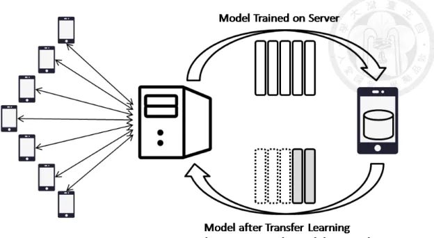
In this paper, we propose a framework to make this model improvement process much more efficient. The proposed framework first trains a model on server with available data. We assume that we do have sufficient data to train a reasonably good model.

However, we still want to make it more robust. As a result, we collect new data from mobile devices, then improve the models by training them locally on the mobile devices.

The mobile devices will train the models with newly collected data via transfer learning, which reduces the computational complexity and the training time. Finally, the mobile devices will send their improved models back to the server. We will get more accurate predictions by combining the predictions from all these models together. This framework also preserves user privacy since only the improved model is sent to the server, instead of private user data. Please refer to Figure 1.1 for an illustration of the proposed framework.

The proposed framework is based on federated learning [27]. The essential difference between our framework and traditional federated learning is how we group the models from mobile devices. Our framework does not aggregate all the models into a single one.

Instead, these models will vote according to their prediction, and achieve a final prediction.

(14)

Figure 1.1: The architecture of the proposed framework

In this paper we consider two voting mechanism – plurality voting and bicameralism voting. Plurality voting is an intuitive and easy method, and has been studied in the liter- ature [3, 22, 29]. We propose bicameralism voting, a new method in combining various results from different models.

1.3 Contribution

The main contribution of this paper is bicameralism voting, which has three advantages. First, from our experiments bicameralism voting achieves higher accuracy than the model trained directly with all the data. Here ”all the data” include the original data on the server and the new collected data from the mobile devices. We believe that this better accuracy, over a single model, comes from the diversity of different models. In addition to better accuracy, bicameralism voting is faster than training a complete model. Finally, federated learning has a constraint that the models to be grouped together must have the same architecture, the same input data preprocessing, and the same format of model. Oth-

(15)

erwise we will have different number of weights and/or different scale of weights, which make grouping impossible. That is, it is not feasible to just average the weights without the risk of ruining the model. In contrast bicameralism voting does not have this limita- tion. As long as each model provides its classification result and the probability of this result, we are able to conduct a voting.

In addition, we try to use this framework to make applications. Bicameralism voting is more suitable as an intermediate product rather than the final product because the process of inference is complicated. In order to make it easy for users, we should still work on enhancing a single model. To enhance a model, we must have more training data. When doing a machine learning, the most difficult part is often to obtain a lot of labeled data. It’s relatively easy to get unlabeled data such as from Internet. Therefore, we want to use unlabeled data to enhance models through our framework. The key point is how to generate labels to the unlabeled data. We will generated labels of unlabeled data via bicameralism voting, and used these labels to enhance original models. The benefits of this framework is that we can make good use of private photos on mobile devices without violating the privacy of owners of mobile devices. With the help of data on mobile devices, the model on the server can make better predictions for unlabeled data, but that data doesn’t need to be delivered to the server. Bicameralism voting can increase the accuracy of predictions efficiently, which makes the generated labels more useful.

In this paper we also present the simulation results of our proposed framework. We will simulate all the interactions between the server and the mobile clients in our framework, with techniques like data segmentation and transfer learning. Also we will show the results when we use the unlabeled data to enhance our models. In the experiments, we try to do that in different situations and under different data partition methods. The training

(16)

on the mobile devices will be simulated by various programs running on the server.

1.4 Overview

We use Food-101 [6] dataset in our experiments because we believe that food recognition is important in our daily life. Nowadays, people take pictures of food with their mobile phones quite often. As a result, there will be plenty of pictures of food available on mobile phones. Since pictures of food are easily obtainable on mobile phones, they can serve as the new (training) data for the models on the mobile devices in our framework.

In order to recognize food accurately, we use convolutional neuron network, which is very effective in image classification. In particular, we choose a famous and simple model, VGG-19, as the neuron network model in our framework.

The remainder of this paper is organized as follows. Chapter 2 piesents the related works. Chapter 3 describes the background of federated learning. Chapter 4 describes our proposed framework. Chapter 5 describes the setting of our experiments and evaluates our framework. Chapter 6 summaries our works and gives possible future works.

(17)

Chapter 2 Related Works

In this chapter, we will briefly introduce related papers on deep learning and federated learning.

Convolutional neural networks(CNN) have been widely used in deep learning since LeNet and AlexNet was proposed [21]. In recent years, computer scientists have proposed many different CNN model architectures, including VGG, Inception, ResNet, MobileNet, and so on [9,16,18,36–39].

Traditional deep learning methods require the training data to be concentrated on one machine, resulting in a limited model size and long training model time. Distributed deep learning solves network size limitations and reduces the time required to train models.

Federated learning is a distributed deep learning approach that trains decentralized data across multiple mobile devices. Each mobile device uses its own private data training model, and then the server combines the global model by averaging the local gradients of each mobile device’s model. Since the mobile device user did not upload the private data to the server, federated learning can reduce privacy risks and reduce the amount of data that needs to be stored on the server [34]. By using large amounts of data on mobile devices, federated learning can train high quality models [27].

There are still several problems with federated learning. For example, the network

(18)

connection between the server and each client is usually slow and unreliable. Konecný et al. [20] proposes two ways to reduce the cost of uplink communications by two orders of magnitude. Zhu et al. [45] uses a multi-objective evolutionary algorithm to minimize communication costs.

A new federated learning protocol FedCS is proposed by Nishio et al [30]. When some clients require longer update time or longer upload time, FedCS can actively manage clients to perform federated learning efficiently.

Another problem is that federated learning is vulnerable to various attacks, such as one of the models to mis-classify a set of chosen inputs with high confidence. Bhagoji et al. [4] and Geyer et al. [14] tackles this problem.

Computer scientists have also proposed many applications based on federated learning. Hard et al. [15] uses federated learning to implement Next-word prediction in a vir- tual keyboard for smartphones. Chen et al. [7] introduced the federated meta-learning framework for training and deploying recommendation systems. Kim et al. [19] proposes a blockchained federated learning architecture. Most of the works aggregate the results from clients for updating the model on the server [5,7,15,20,25,27,28].

The objective of these works are speeding up the training process by distributing the workload or dataset among multiple clients. A server is used for coordinating the gradients from these clients.

In this paper, we consider the result acquired from each client individually. Each client uploads its local model to the server instead of uploading the gradient. Then the server combines these models by voting.

(19)

Chapter 3 Background

The framework proposed in our paper is based on transfer learning and federated learning.

3.1 Transfer learning

Transfer learning is a technique in machine learning. Transfer learning stores the knowledge it has learned while solving a source task and apply the knowledge to a target task [13,24,31,40,41,44]. The target task must be similar but not identical to the source task.

In a convolutional neural network using the concept of transfer learning, we pre-train a model on the data set of the source task. To store the knowledge learned on the source task, we keep the weights of the convolution layer and freeze them. The weights of the fully connected layer are then randomly initialized and retrained on the data set of the target task. In this way, the network will use the stored knowledge to solve the target task.

3.2 Federated learning

Federated learning is a distributed machine learning approach [27], first proposed by

(20)

McMahan et al. A federated learning system includes a server and multiple mobile device clients. Each client has its private data, such as photos, which is often privacy sensitive.

The purpose of federated learning is to use these decentralized data across multiple mobile devices for machine learning without intruding privacy.

Unlike traditional machine learning, federated learning does not require client to upload private data to the server for training. Instead each client trains a model with its own data. In addition, each client uploads the gradient of its model to the server during its training, and the server combines these gradients by averaging them, and builds a global model. Federated learning enables model training on a large corpus of decentralized data, and the data will never leave the client to preserve privacy.

Federated learning uses random gradient descent to update the model, which is an optimization technique for updating model parameters. The random gradient descent is an iterative method that repeatedly calculates the gradient of weights and improves the network during the optimization process.

Although random gradient descent is often used for machine learning, it is not suitable for federated learning. The reason is that the gradient calculation is done by the clients, and after each round of gradients computation, the server must retrieve the gradients from the clients and combine them to improve the global network. The global network is then sent back to the clients before the next round of calculations. Due to this repeated uploading and downloading of gradients, the network between the clients and the server must have low latency and high throughput, which is not always possible in a federated learning environment.

In this paper, we propose a framework that combines federated learning and transfer

(21)

learning so that communication between the client and the server is only required when uploading and downloading the model. Our framework reduces the amount of communication, solves the communication problems of federated learning, and improves the accuracy of the global model.

(22)

Chapter 4 Methods

The roles of convolution layers and fully connected layers of a network are very different in transfer learning. In a convolutional neuron network (CNN) model, the convolution layers are for general feature extraction, so they will not be affected during transfer learning. On the other hand, the fully connective layers are more related to the categories of input data, and will be affected during transfer learning. That is, the convolutional layers will not be affected by the newly added input data, and the model will still be able to adapt to the new data by changing the weights in the fully connected layers.

Our framework adopts voting, instead of federated aggregation in traditional approach, to predict the final answer. Due to the limited amount of data each mobile device could use to train the model, the resulting model will be diverse, and may even be over- fitting. Nevertheless, we decide to let these models vote for the final prediction, instead of using federated aggregation. That is, federated aggregation averages the weights of all models, which effectively eliminates the diversity of various models trained on the mobile devices. On the other hand, voting lets the model express their own opinions.

It is essential to consider the confidence of the voters in a voting process. When given an input, a model will predict two things – the classification result and confidence (a probability) it has in its prediction. We will consider two types of voting based on this

(23)

confidence – plurality voting and bicameralism voting. Both voting methods utilize the knowledge learned on mobile devices for federated learning.

4.1 Plurality Voting

We consider four types of plurality voting for models to vote.

4.1.1 Majority Vote

Given a set of votes, the majority vote is the simplest plurality voting to decide the final result. Every model votes for their prediction, and the class having the highest number of votes will be the final result.

4.1.2 Confidence Vote

We propose a confidence vote for models to vote. In a confidence vote, every model casts a vote, which has a weight of the confidence of that prediction. That is, if a model has confidence of c in its prediction, it will vote and its vote has a weight c. The final result will be the class having the highest sum of weights, i.e., the confidence.

4.1.3 Majority Vote with Confidence Threshold

We also propose a majority vote with confidence threshold for models to vote. We set a confidence threshold α so that only models having confidence at least α can vote, and their votes are all of the same weight, like in a majority vote. That is, if we set the α to 0, majority vote with confidence threshold just becomes majority vote. The rational

(24)

for this approach is that we will let models vote only when they have good confidence.

In addition, we do not wish to see the case where a large number of low-confidence votes dramatically change the voting result.

4.1.4 Confidence Vote with Confidence Threshold

We finally propose a confidence vote with confidence threshold for models to vote.

That is, only the models having high confidence can vote (like in majority vote with confidence threshold), and the weight of their votes are the confidence of their prediction (like confidence vote).

In both majority vote with confidence threshold and confidence vote with confidence threshold, we need to choose a threshold. Therefore, we conduct experiments to find good threshold values. We let every model make predictions for all test data, and we calculate the average probabilities of correct predictions and wrong predictions. Then, we use the value between the average of the probabilities of correct and incorrect predictions as the threshold.

4.2 Bicameralism Vote

In plurality voting described in the previous section, the model trained at the server was never used in the prediction. We will denote this model as the master model. The master model is simply transferred to the mobile devices in order to provide good convolutional layers, and then trained into various student models on the mobile devices.

We observe that the prediction accuracy of the master model is better than any single

(25)

student model. In addition, after group all the student models together by naive plurality voting, the overall prediction accuracy of the student model is still inferior to that of the master model. As a result, we would like to build a framework that will leverage the synergy of both the master and the student models, so that the prediction can be more accurate than either approach.

Classification result Average probability

Student models

Crowd model Input data

Input data

Master model

Crowd model

Final result Compare their

probability

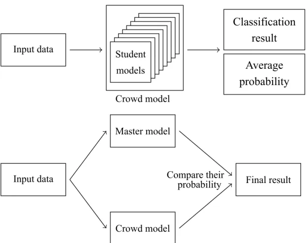
Figure 4.1: Bicameralism. Production of crowd model, and prediction making.

For ease of explanation we will use a crowd model to denote the collection of student model. Recall that a prediction consists of a classification result and the probability (i.e., confidence) that the model believes in the result. In our framework every student model makes a prediction for one input data, as shown in Figure 4.1 shows. And then student models will collectively predict a result with confidence vote with confidence threshold described earlier. That is, if a model has a confidence higher than a threshold, its vote will have the confidence as the weight. The class having highest total confidence is the

(26)

classification result, with a confidence set to the average confidence of these models vote for it. This combined model will be referred to as the crowd model.

We now propose bicameralism vote. After combining the student models into a crowd model, we then predict with the crowd and the master model individually. Both the master model and the crowd model will make a prediction for an input data, we then compare the confidence of the two model, and choose the one with higher confidence.

In bicameralism vote, the importance of the master model and the crowd model are the same. Experiment results indicates that this is a reasonable ratio of the importance of the master model participation in voting. If the master model participates plurality voting as other students do, its influence will be minimum.

In practice it will be difficult to find a good ratio for the importance of the master model. In some cases, if we increase the ratio of the master model, the accuracy will be even better than a simple bicameralism vote. However, the best ratio may eventually have to be determined by a brutal force search. Thus, without any prior knowledge, the bicameralism vote is a simple and reasonable way to balance the importance between the master and the crowd model.

We observe that in bicameralism vote, the importance of the master model should be determined by its robustness. If a master model is robust enough, the result from the crowd model will be simply a helper. On the other hand, a crowd model can improve the classification results of a poor master model.

(27)

4.3 Application

Although the accuracy of bicameralism is high, the result of a prediction comes from master model and many student models, which is complicated. Even if the part of predictions from student models can be parallelized or distributed, bicameralism is still too cumbersome to be a application for users directly. Therefore, we proposed a framework to make use of bicameralism. We can generate labels of unlabeled data through bicameralism, and put these new data into training process to enhance master model.

First, we train master model with labeled training data. After that, we generated many student models from master model. Master model and student models make predictions to the unlabeled data through bicameralism. We treated these predictions as labels for the unlabeled data and put them together with training data of the master model. Then we retrained master model with the original training data and the new labeled data. A new group of student models were generated from the updated master model. They make prediction to the unlabeled data through bicameralism again. The accuracy of predictions to the unlabeled data would be improve through the second round of bicameralism. And also these unlabeled data could enhance master model. The process can be repeated to improve master model.

Note that there are two different situations when saying the unlabeled data. The first one is repeating the same unlabeled data. If the situation is that you only collect one set of unlabeled data, you can keep using these unlabeled data to do above process. Due to the improvement of the predictions to the unlabeled data, these unlabeled data still can enhance master model in second or third round. That is, we maximize the value of these unlabeled data. The second one is to put unlabeled data in batches. If we kept collecting

(28)

unlabeled data, we could put the existing unlabeled data in every time. When the amount of one batch is not so much, every time we do bicameralism to make predictions on new batch and all the previous batches. The accuracy of previous batches of unlabeled data can be improve, therefore master model will has more accurate knowledge from unlabeled data.

In practice, the labeled data we have initially may be few. The accuracy of the predictions on unlabeled data will be low even if doing bicameralism voting. That is, there will be too many noises in the unlabeled data to treat the they as training data. Therefore we add a filter to delete some useless unlabeled data, which makes the accuracy of labels generated by bicameralism higher.

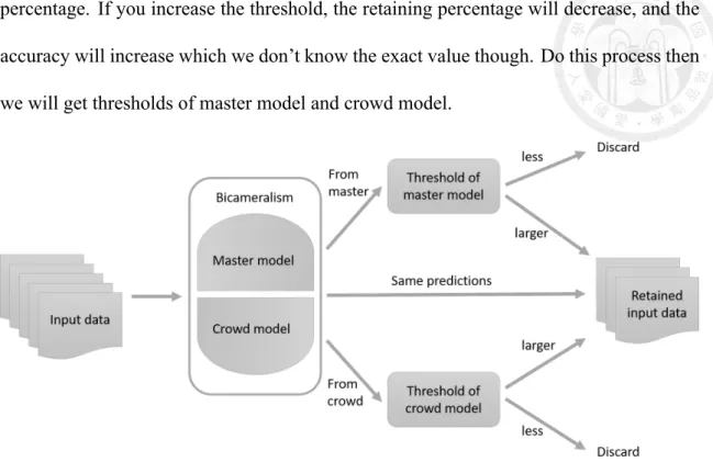
The following part will show the detail of filter, and it is also shown in Figure 4.2.

The predictions from bicameralism come from master model and crowd model actually. If master model and crowd model make the same prediction on one input, then this input will be retained. Because the accuracy is high if master model and crowd model have the same opinion. If the prediction comes from either master model or crowd model, its confidence of prediction should higher than a threshold, or it won’t be retained. Master model and crowd model have a threshold respectively. We do bicameralism on test data first. Note that we know the labels of test data because they come from labeled data. Then we find out the average confidence of correct predictions of master model and average confidence of wrong predictions of master model. The base threshold of master model is the average of correct average confidence and wrong average confidence. We use this base threshold to filter the unlabeled data and fine-tune the threshold. We can only know the percentage of the retaining inputs after filtering, and can’t know the accuracy of the retaining inputs after filtering because they are unlabeled data. We can fine-tune the threshold by retaining

(29)

percentage. If you increase the threshold, the retaining percentage will decrease, and the accuracy will increase which we don’t know the exact value though. Do this process then we will get thresholds of master model and crowd model.

Figure 4.2: How does a filter work.

(30)

Chapter 5 Evaluation

5.1 Evaluation Settings

We first describe our experimental environment. Our proposed framework should have a server and a large number of mobile devices. However, due to the limited number of mobile devices we have, we simulate the training and inference processes of these large number of mobile device on a server, which has 64 GB RAM and a GeForce GTX 1080 GPU card with 8 GB memory.

We train both the master and student models on the GPU one at a time. Since this paper focuses on improving the accuracy, instead of speeding up training time, it is reasonable to train the student models on a server with a more powerful GPU than actually using the GPU on a mobile device. That is, this is a feasibility study, rather than a performance study.

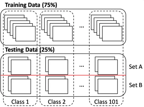
The experiments use Food-101 [6] dataset. Food-101 is an image dataset containing 101 food classes, and each class has 1,000 images. For each class, there are 750 training images, and 250 manually reviewed images for testing. That is, there are noises in training images and no noise in testing images.

We use the training data to train the master model on the server. We randomly divide

(31)

the test data into two equal size subsets – A and B. The set A is used as the training set for the student models on mobile devices, and the set B is used to evaluate accuracy. Please refer to Figure. 5.1 on how the dataset is partitioned, and to what training purpose.

Figure 5.1: Data set used in training the master and the student models

We use VGG-19 [36] as the model in our experiment. VGG-19 is a convolution neuron network for large-scale image recognition. A VGG-19 network has 16 convolutional layers and 3 fully-connected layers. We chose VGG-19 because it is easy to obtain, easy to maintain, and powerful enough for image recognition.

We use TensorFlow [1] to train VGG-19 model to obtain the master model and student models. TensorFlow is one of the state of the art deep learning training platform and we are very familiar with it, and we are able to develop simulation programs quite quickly with it.

(32)

5.1.1 Master Model

We train the master model from scratch, i.e. we start with a set of random initialized weights in the VGG-19 model. This is a standard procedure since we do not have any prior knowledge about the VGG-19 model nor the Food101 dataset.

We then use the entire training data of Food-101 to train the master model. The reason we use the entire training set is to improve the quality of the convolutional layers of VGG-19 in the master model. Note that the quality of convolutional layers is essential to prediction accuracy. In addition, the convolutional layers will be frozen after they are transferred to the mobile device as the part of the the student model, so we must guarantee the quality of these layers, which will significantly affect the final prediction.

We tried to reduce the amount of training data down to 20% and 37% of the entire dataset while training the master model. However, the convolutional layers of the resulting models cannot provide sufficient information, i.e. extract meaningful features, for the fully-connected layers during transfer learning.

The training of the master model takes about one weeks before it converges on the entire training data of Food-101. The accuracy of the master model reaches 73.60% for the union of test set A and B, and 73.06% for test set B only.

5.1.2 Student Models

We assume that there are 150 mobile devices in our evaluation. Each user device receives a pre-trained master model from the server, and 13 randomly chosen data from each class of set A. This amount of these data is only about 1.3% of the entire dataset,

(33)

which is a very small amount.

We simulate the case that each mobile device performs transfer learning using the set of images on the device to generate a student model. Note that since the data on each device will be different (they are randomly chosen from set A), the weights of the fully- connected layers of different student models will be different.

5.2 Comparison between Methods

We examine the performance of our proposed bicameralism voting. Recall that bicameralism vote makes decisions based on the results from the master model and the crowd model. The decision of the crowd model is the plurality of all the student models.

Each student model is fine-tuned from the master model using transfer learning with part of the images in set A as the training set. The confidence threshold of the crowd model of bicameralism is set to 0.

We compare the accuracy of the bicameralism voting with other methods. Since the total percentage of data seen by bicameralism voting (both master and student models) is 87.5%, the most intuitive comparison baseline is a single model trained with the same amount (87.5%) of data. Therefore, we fine-tune the master model with extra data, and use the erudite model to denote it. The training data of erudite model includes the training set of the master model and the subset A.

Model Accuracy

Bicameralism 77.838%

Master 73.061%

Erudite 75.517%

Table 5.1: Accuracy of different models.

(34)

Table 5.1 shows the accuracy of the master model, the bicameralism model, and the erudite model. Note that the test data is the subset B, and none of these models has prior knowledge about it.

We conclude from Table 5.1 that both the erudite model and the bicameralism model perform better than the master model because it was trained with a larger training set.

Surprisingly, the bicameralism model achieves better accuracy than the erudite model, based on the the same amount of training data. The authors believe that the synergy of the high accuracy of the master model and the diversity of the crowd model help achieve this high accuracy.

The bicameralism model has the additional advantage of efficiency. Given the master model, it takes about a week for the erudite model to converge on a server in our experiment. On the other hand, the training of crowd models (all the student models) in bicameralism can complete in 25 hours.

5.2.1 Weighted Plurality Voting

We compare the accuracy of Bicameralism model with that of weighted plurality vote. In a weighted plurality vote, the master model also votes like every student model does, but with a weight.

We implement two types of weighted plurality votes. The first is the majority vote with the master. That is, each student model can cast one vote, just like the majority vote in Section 4.1.1, and the master can cast w vote, where w is the weight of the master. The second is the confidence vote with the master. The value of a vote from a student is its confidence, just like in the confidence vote in Section 4.1.2, and the value of a vote from

(35)

the master is its confidence multiplied by its weight.

0.66 0.68 0.7 0.72 0.74 0.76 0.78 0.8

0 10 20 30 40 50 60 70 80 90 100 110 120 130 140 150

Accuracy

Weight

vote(probability) vote(one)

Figure 5.2: Accuracy of the Weighted Plurality Vote

Figure 5.2 shows the accuracy (in y axis) of majority vote with the master, and confidence vote with the master, using different weights (in x axis) for the master model.

We observe that confidence vote with the master achieves higher accuracy than majority vote with the master under all weights. The confidence vote with the master achieves its highest accuracy when weight is 93, then the accuracy saturates. The majority vote with the master achieves its highest accuracy also when weight is around 93. However, the accuracy begins to decline after that.

We conclude from Figure 5.2 that finding a suitable weight for the master is not trivial, and can be application-dependent. On the other hand, the bicameralism model is a good choice for two reasons. First, it achieves 77.838% accuracy, which is only slightly lower than the best weighted plurality votes in Figure 5.2. Second, we do not need to find

(36)

a good weight for the master model.

5.3 Improvement Analysis

In this section, we analyze why the bicameralism model has better accuracy. The threshold of crowd model is 0. From Section 5.2 we observe that the bicameralism model achieves better accuracy than erudite model does, using the same amount of training data.

tests (percentage) accuracy master & crowd 8147 (64.53%) 92.39%

master 2054 (16.27%) 61.54%

crowd 2424 (19.20%) 42.74%

total 12625 (100%) 77.838%

Table 5.2: # of inputs two models agree/disagree, and the accuracy

We divides the prediction results into three categories in Table 5.2. The row master

& crowd indicates the case where the two models make the same prediction. The row master (crowd) indicates the case where the two models have different predictions, and the master (crowd) model has a higher confident value.

We observe Table 5.2 that if the master and the crowd model agree on a prediction, the accuracy is very high. That is, there are 12625 predictions in total, among which for 8147 (64.53%) of them two models make the same prediction, and the accuracy of these predictions is 92.39%. On the other hand, when the two models disagree on an input, the one with higher confidence will be chosen. In other words, the crowd model is complementary to the master model, therefore it can help improve the overall accuracy.

(37)

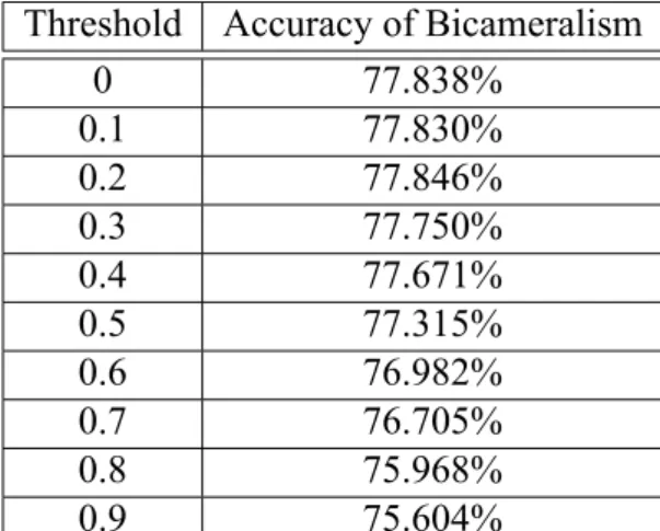
5.4 Impact of the Confidence Threshold

We now evaluate how confidence thresholds affects the accuracy of the bicameralism voting. Recall that only models having confidence over a threshold can vote in these cases.

In this experiment, we test the confidence vote with confidence threshold.

Threshold Accuracy of Bicameralism

0 77.838%

0.1 77.830%

0.2 77.846%

0.3 77.750%

0.4 77.671%

0.5 77.315%

0.6 76.982%

0.7 76.705%

0.8 75.968%

0.9 75.604%

Table 5.3: Different confidence thresholds and the corresponding accuracy

Table 5.3 lists the confidence thresholds and the corresponding accuracy of bicameralism voting. Surprisingly we observe that the accuracy decreases as the confidence threshold increases. Our initial guess is that setting a higher threshold for the student models to vote should improve the accuracy because only those models with high confidence will vote. However, from the experiment, this may not be the case.

The reason for this unexpected behavior may be that the diversity from a low threshold actually improves prediction. There could be cases that a large number of models are able to predict the correct results, but with little confidence. A high threshold will simply ignore their opinions, and the vote will be dominated by those models that have high confidence, which may not be correct after all. Therefore, We suggest not to set a threshold (threshold = 0) as the default setting when no prior knowledge is available.

(38)

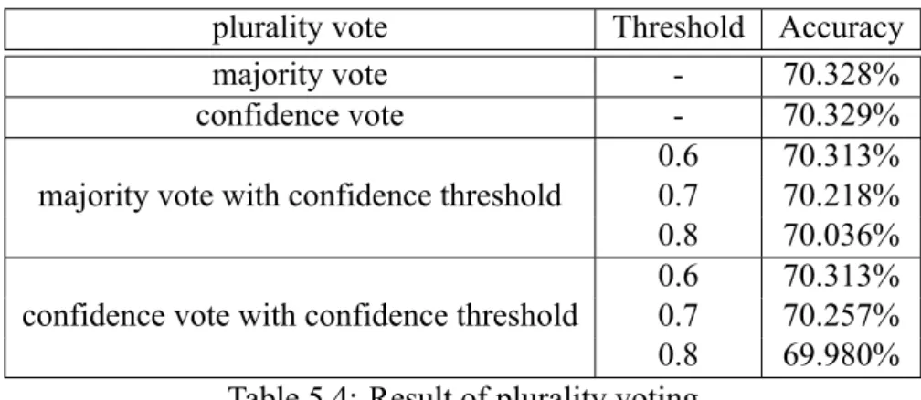
5.5 Different Implementations of the Crowd Model

Table 5.4 compares the accuracy of the four plurality voting described in Section 4.1.1.

We set the threshold from 0.6 to 0.8, because we found that the average confidence of a correct and incorrect prediction are 0.87 and 0.54 respectively. As a result we set the threshold in between 0.87 and 0.54, i.e., a value higher than 0.87 would stop models making correct prediction from voting, and a threshold lower than 0.54 would likely allow models making wrong prediction to vote.

Table 5.4 indicates that all four plurality voting methods have almost the same accuracy, and confidence vote is slightly higher than the others. This indicates that limit voting with threshold does not have apparent advantage.

plurality vote Threshold Accuracy

majority vote - 70.328%

confidence vote - 70.329%

majority vote with confidence threshold

0.6 70.313%

0.7 70.218%

0.8 70.036%

confidence vote with confidence threshold

0.6 70.313%

0.7 70.257%

0.8 69.980%

Table 5.4: Result of plurality voting

5.6 Influence of the Student Models

We now discuss the impact of different hyper-parameters and settings on training the student models. Recall that a student model is fine-tuned from the master model with transfer learning using a small amount of data on the mobile device. We use three different sets of hyper-parameters to train the student model. We also consider the possibility of

(39)

updating both convolutional and fully-connected layers during the transfer learning. The confidence threshold is set to 0 in this experiment, as indicated in previous experiments that having a threshold does not have apparent advantage.

Table 5.5 shows the average accuracy of the student models and the bicameralism model. We observe that the accuracy of bicameralism model decreases when the the average accuracy of the student models increases. The reason is that when the average accuracy of the student models increases, they become more and more similar to the master model.

In other words, the diversity we expect from having multiple models gradually disappears when the student models are just like the master model. The accuracy of the bicameralism model will simply converge to the accuracy of using only the master model, which is 73%.

We also observe that updating the entire model, including the convolution layers, does not provide better accuracy, than updating only the fully connected layers, like in ordinary transfer learning. We observe this in both the student models and the bicameralism model.

The reason is that the amount of data on each device is relatively small and might be biased.

Changing the convolutional layers with biased data will not help the accuracy.

Method Setting

Avg. Accuracy of the Student Models

Accuracy of Bicameralism Transfer

Learning (Freeze Conv. layers)

Learning Rate:0.025

# of epoch: 50 61% 77%

Learning Rate:0.01

# of epoch: 50 65% 76%

Learning Rate:0.0001

# of epoch: 50 71% 73%

Fine-tune the entire

CNN

Learning Rate:0.001

# of epoch: 50 60% 73%

Table 5.5: Average accuracy of the student and the bicameralism model

(40)

5.7 Improvement by Unlabeled Data

We re-partition Food-101 dataset into four parts for these experiments because the amount of data is limited. The four parts are training data, unlabeled data, students’ data and test data respectively. And the percentages of them are 35%, 30%, 10%, and 10%

respectively. Training data is used for training master model. Unlabeled data will get their labels through predictions from bicameralism and become the training data of master model. Students’ data is used for training all the student models. Test data is used to evaluate the quality of models.

Note that the training data and the test data here are the different subset of Food- 101 from the previous bicameralism voting part, so the accuracy of models of this part is different. In bicameralism voting part, we partition the data into training data and testing data according to the way recommended by the author of Food-101. There are no noises in these test data. In this part, we sorted images by their names in all the classes of Food-101 respectively, and take the top N% data When we need N% data. The test data is always the last 10% and there are noises in these test data.

Test data Unlabeled data

Master model Bicameralism Master model Bicameralism

1st 62.42% 66.30% 62.28% 66.30%

2nd 64.09% 68.19% 66.13% 67.81%

3rd 64.96% 68.68% 66.82% 68.60%

4th 65.73% 69.80% 67.74% 69.46%

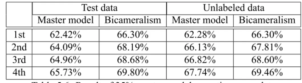
Table 5.6: Result of 35% master model repeating same data

Table 5.6 shows the result of the first situation of unlabeled data. That is, bicameralism makes predictions on all the unlabeled data(35%) at once, and they will be a part of training data in next round. The first row in Table 5.6 is the result of the first round, and

(41)

the second round in Table 5.6 is the result of the second round and so on. In first round, training data(35%) was used to train master model. In second, third, and fourth round, both training data(35%) and unlabeled data(30%) were used to train master model. The accuracy of the generated labels of unlabeled data is the accuracy of bicameralism of unlabeled data in the previous round. That is, the fourth column. Test data is used to test the robustness of the model, on the other hand, unlabeled data are used to show the quality of generated labels. As we can see, the accuracy of bicameralism of unlabeled data increased every round. Therefore master model can receive more information from the unlabeled data.

1st 62.42% 66.30% 62.20% 65.64%

2nd 64.66% 68.67% 65.04% 68.21%

3rd 64.92% 69.19% 67.66% 69.84%

4th 65.74% 69.63% 69.14% 70.18%

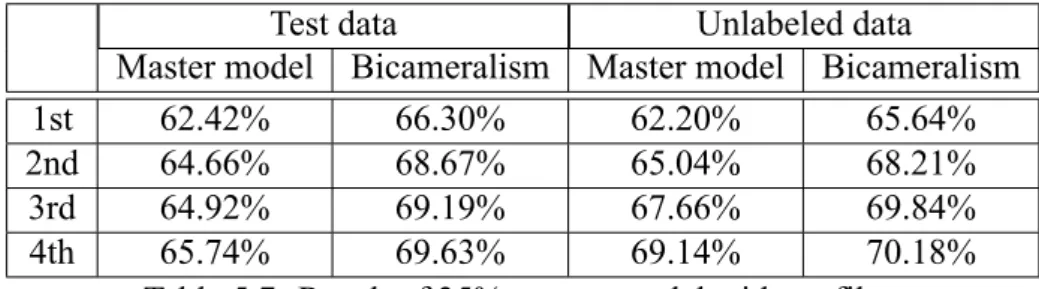
Table 5.7: Result of 35% master model without filter

Table 5.7 shows the result of the second situation of unlabeled data. In first round, training data(35%) is used to train master model, too. In the next three rounds, one-third of unlabeled data(10%) is added to the training data every round. When the fourth round, all the unlabeled data is added to the training data. In third or fourth round, the original unlabeled data would be re-predicted as well as newly added unlabeled data. The fourth element of the first row is the accuracy of first one-third of unlabeled data, and the fourth element of the second row is the accuracy of first two thirds of unlabeled data. The fourth element of the third and fourth rows are the accuracy of all of unlabeled data. The results show that the final effect to master model of two situations of unlabeled data are almost the same. However, the second one is more efficient because when the second and third round, less unlabeled data was added to the training data. The amount of computation

(42)

would be less.

1st 62.42% 66.30% 62.20% 65.64%

2nd 64.29% 69.16% 66.17% 69.68%

3rd 65.42% 70.32% 68.83% 71.44%

4th 66.37% 70.70% 70.00% 71.96%

Table 5.8: Result of 35% master model with filter

Table 5.8 shows the result of the second situation of unlabeled data with filter. The usage of unlabeled data here was same as previous part, One-third of unlabeled data was added each round. We used the filter to decrease the noises in unlabeled data, so master model would obtain more useful data. The amount of added unlabeled data would cut back but it was good for quality of training data and training efficiency. As we can see the result is better than all the previous parts. Our master model in the fourth round used 65%

data of Food-101, and its accuracy is up to 66.37%. Although the accuracy of a model using 65% data of Food-101 is 68.55%, our master model used only 35% real labels.

Round Accuracy

Percentage of Retaining

Input

Saving Time Second

Round 79.69% 74.72% 2.4hr (5.7%) Third

Round 79.97% 82.00% 5.0hr (6.7%) Fourth

Round 82.14% 80.36% 3.8hr (9.3%) Table 5.9: Detail of Filter

Table 5.9 shows the detail of the filter. From the second round, unlabeled data was added, so this table displays the detail from the second round. After filtering the generated labels of unlabeled data, those whose confidences were higher than the threshold would be retained. The third column, Percentage of Retaining Input, means that the percentage of unlabeled data whose confidences were higher than the threshold. The second column,

(43)

Accuracy, means the accuracy of retained unlabeled data. We can see that the accuracy is significantly increased after passing the filter. After the useless data was deleted, the amount of computation for master model training was reduced. The computation time was reduced too. The fourth column, Saving Time, means that how much time was saved compared with the one without filter.

1st 56.26% 60.50% 56.17% 61.28%

2nd 57.94% 61.67% 59.84% 62.53%

3rd 57.36% 61.60% 62.14% 62.70%

Table 5.10: Result of 20% master model without filter

1st 56.26% 60.50% 56.17% 61.28%

2nd 58.69% 62.85% 61.05% 64.00%

3rd 59.81% 63.50% 64.00% 65.06%

Table 5.11: Result of 20% master model with a filter

Besides doing the experiment from the 35% master model, we also did it from the 20% master model. The 35% master model means that the master model used 35% labeled data, and started to add unlabeled data in. Now, we want to try the experiment from a weaker master model, 20% labeled data used only. Table 5.10 shows the of 20% master model without filter, and Table 5.11 shows the of 20% master model with a filter. There was 10% data added to the master model in both the second and the third round. If we didn’t use a filter, then the accuracy of predictions of unlabeled data was the result of bicameralism. That is, the number in the fourth column, about 62% only. After using a filter to delete useless data, 73% of inputs were retained and the accuracy of the predictions of unlabeled data was increased to 75.6% in the second round. In the third round, 73% of inputs were retained and the accuracy was increased to 78.3%. Comparing the two tables, we can see that the result of that with a filter is better than that without filter obviously.

(44)

Especially the third round, the result is almost same with the result of the second round.

The result of predictions of unlabeled data through bicameralism was improved very little after the first round. Therefore in the third round, the labels of unlabeled data were almost the same with the previous round. The unlabeled data can no longer improve the master model after the second round.

When the master model is weak, a filter becomes important. The results of the 35%

master model are good whether when it has a filter or not. However, when the predictions to the unlabeled data were not good enough, it needed a filter definitely. But we still recommend using a filter when doing this experiment, because a filter not only improves the result but also speeds up the training.

N% Data Accuracy of master model

10% 28.18%

20% 56.26%

35% 62.42%

45% 67.35%

55% 66.19%

65% 68.55%

75% 68.16%

80% 70.53%

Table 5.12: Different percentage of data and the corresponding accuracy

Table 5.12 shows that using N% data to train a model then the accuracy of the model on the test data. The model here was trained by labeled data. This table can be used as a reference for unlabeled data experiments. For example, the accuracy in the fourth row, the first column of table 5.8 means that using the 65% data to trained a master model.

But in this 65% data, 35% data was labeled data and 35% data was unlabeled data. The accuracy in table 5.8 is a bit lower than the accuracy of 65% model in Table 5.12. On the other hand, the accuracy in the third row, the first column of Table 5.11 is much lower than the accuracy of 45% model in Table 5.12. We think that the master model has to robust

(45)

enough initially, or unlabeled data can’t play a good role.

5.8 Summary

Among all methods we studied, the bicameralism voting and weighted plurality voting have the highest accuracy. However, the bicameralism model is much more feasible in practice. The crowd model is complementary to the master model and can improve the final accuracy. In addition, if we do not properly set the confidence threshold of crowd model, it may not help the accuracy, due to decreased diversity of the student models.

For example, both Table 5.3 and Table 5.4 indicate that setting threshold does not help.

Table 5.5 also indicates that the diversity of student models is essential, because when the student models are more similar to the master model, the accuracy of the bicameralism vote will actually decrease. When we get new unlabeled data and want to improve our model through them, we can general labels by bicameralism voting if our model is not bad originally. Using a filter when adding unlabeled data to re-train a model is a efficient and better way. If you pay great attention to accuracy, you can still use bicameralism voting to make predictions after adding unlabeled data in.

(46)

Chapter 6 Conclusion

In this paper, we propose a bicameralism voting framework to improve the accuracy of deep neuron networks and the training efficiency. Then we use bicameralism voting framework to label unlabeled data and enhance a model.

We first train a master model on a server, then we send the master model to multiple mobile devices, and each of them use its own data to update the master model into its student model by transfer learning. Then the master and the student model uses bicameralism voting to classify inputs.

The bicameralism model has three advantages. First, the bicameralism model has better accuracy than a single model that use the same amount of training data. Second, the bicameralism model is computationally efficient for two reasons. First, transfer learning saves time computation because it improves upon an existing good model, and do not build the model from scratch, so it has less computation. In addition, the computation on the mobile devices can be done in parallel, which can further reduce the transfer learning time. The third advantage of the bicameralism model is its flexibility in how to train the student models. Because we only care about the prediction made by the student models in bicameralism model, how these student models are trained is up to the users. The users can use whatever data preprocessing, architecture, or model format to train the student models.

(47)

As a result it is much more flexible than the federated learning [27], which cannot combine models in different model formats, model architectures, or preprocessing of input data.

The bicameralism model is like a union of the master model and the crowd model, and it selects the prediction from whoever has a higher confidence. Although each student model has a low accuracy individually, their diversity actually helps bicameralism voting in achieving better accuracy. The master model is already a good model by itself, and with the help from a complementary crowd model, the final accuracy of the bicameralism model reaches 77.838%, which is higher than the master model and surprisingly, the erudite model. With bicameralism voting, the predictions we make are more accurate, so we try to generate labels for unlabeled data and improve our master model. With a filter when training, the final result will get a not bad accuracy, just a little bit lower than the one trained by labeled data.

6.1 Future works

We simulate the training of student models in a server (not on multiple mobile devices), due to the large number of mobile devices required by the framework. In the future, we wish to conduct the training of the student models on the mobile devices, and actually consider the communication issues that will arise.

The data set Food101 has a large amount of noise in the images. We would like to investigate the possibility of removing the noise with the crowd model in the future. The idea is that the master model is trained on Food101 only. However, the student models are trained with pictures taken by the mobile devices, and are likely to be labeled. Thus, the distribution of training data for the master model and the student model will be different.

(48)

As a result, the crowd model might be able to locate the noise in Food101 images and relabel them.

(49)

References

[1] M. Abadi, A. Agarwal, P. Barham, E. Brevdo, Z. Chen, C. Citro, G. S. Corrado, A. Davis, J. Dean, M. Devin, S. Ghemawat, I. Goodfellow, A. Harp, G. Irving, M. Is- ard, Y. Jia, R. Jozefowicz, L. Kaiser, M. Kudlur, J. Levenberg, D. Mané, R. Monga, S. Moore, D. Murray, C. Olah, M. Schuster, J. Shlens, B. Steiner, I. Sutskever, K. Talwar, P. Tucker, V. Vanhoucke, V. Vasudevan, F. Viégas, O. Vinyals, P. War- den, M. Wattenberg, M. Wicke, Y. Yu, and X. Zheng. TensorFlow: Large-scale machine learning on heterogeneous systems, 2015. Software available from tensorflow.org.

[2] O. Abdel-Hamid, A.-R. Mohamed, H. Jiang, L. Deng, G. Penn, and D. Yu. Convo- lutional neural networks for speech recognition. IEEE/ACM Trans. Audio, Speech and Lang. Proc., 22(10):1533–1545, Oct. 2014.

[3] E. Bauer and R. Kohavi. An empirical comparison of voting classification algo- rithms: Bagging, boosting, and variants. Machine learning, 36(1-2):105–139, 1999.

[4] A. N. Bhagoji, S. Chakraborty, P. Mittal, and S. B. Calo. Analyzing federated learning through an adversarial lens. CoRR, abs/1811.12470, 2018.

[5] K. Bonawitz, H. Eichner, W. Grieskamp, D. Huba, A. Ingerman, V. Ivanov, C. Kid- don, J. Konecný, S. Mazzocchi, H. B. McMahan, T. V. Overveldt, D. Petrou, D. Ra-

(50)

mage, and J. Roselander. Towards federated learning at scale: System design. CoRR, abs/1902.01046, 2019.

[6] L. Bossard, M. Guillaumin, and L. Van Gool. Food-101 – mining discriminative components with random forests. In European Conference on Computer Vision, 2014.

[7] F. Chen, Z. Dong, Z. Li, and X. He. Federated meta-learning for recommendation.

CoRR, abs/1802.07876, 2018.

[8] Z. Chen and D. Yi. The game imitation: Deep supervised convolutional networks for quick video game AI. CoRR, abs/1702.05663, 2017.

[9] F. Chollet. Xception: Deep learning with depthwise separable convolutions. CoRR, abs/1610.02357, 2016.

[10] E. David, N. S. Netanyahu, and L. Wolf. Deepchess: End-to-end deep neural network for automatic learning in chess. CoRR, abs/1711.09667, 2017.

[11] L. Deng and J. Platt. Ensemble deep learning for speech recognition. Proceedings of the Annual Conference of the International Speech Communication Association, INTERSPEECH, pages 1915–1919, 01 2014.

[12] G. Eilertsen, J. Kronander, G. Denes, R. K. Mantiuk, and J. Unger. HDR image reconstruction from a single exposure using deep cnns. CoRR, abs/1710.07480, 2017.

[13] Y. Ganin and V. Lempitsky. Unsupervised domain adaptation by backpropagation.

In F. Bach and D. Blei, editors, Proceedings of the 32nd International Conference on

(51)

Machine Learning, volume 37 of Proceedings of Machine Learning Research, pages 1180–1189, Lille, France, 07–09 Jul 2015. PMLR.

[14] R. C. Geyer, T. Klein, and M. Nabi. Differentially private federated learning: A client level perspective. CoRR, abs/1712.07557, 2017.

[15] A. Hard, K. Rao, R. Mathews, F. Beaufays, S. Augenstein, H. Eichner, C. Kiddon, and D. Ramage. Federated learning for mobile keyboard prediction. CoRR, abs/

1811.03604, 2018.

[16] K. He, X. Zhang, S. Ren, and J. Sun. Deep residual learning for image recognition.

CoRR, abs/1512.03385, 2015.

[17] S. Hershey, S. Chaudhuri, D. P. W. Ellis, J. F. Gemmeke, A. Jansen, C. Moore, M. Plakal, D. Platt, R. A. Saurous, B. Seybold, M. Slaney, R. Weiss, and K. Wilson.

Cnn architectures for large-scale audio classification. In International Conference on Acoustics, Speech and Signal Processing (ICASSP). 2017.

[18] S. Ioffe and C. Szegedy. Batch normalization: Accelerating deep network training by reducing internal covariate shift. CoRR, abs/1502.03167, 2015.

[19] H. Kim, J. Park, M. Bennis, and S. Kim. On-device federated learning via blockchain and its latency analysis. CoRR, abs/1808.03949, 2018.

[20] J. Konecný, H. B. McMahan, F. X. Yu, P. Richtárik, A. T. Suresh, and D. Bacon.

Federated learning: Strategies for improving communication efficiency. CoRR, abs/

1610.05492, 2016.

[21] A. Krizhevsky, I. Sutskever, and G. E. Hinton. Imagenet classification with deep convolutional neural networks. Commun. ACM, 60(6):84–90, May 2017.

(52)

[22] A. Krogh and J. Vedelsby. Neural network ensembles, cross validation, and active learning. In Advances in neural information processing systems, pages 231–238, 1995.

[23] G. Lample and D. S. Chaplot. Playing FPS games with deep reinforcement learning.

CoRR, abs/1609.05521, 2016.

[24] M. Long and J. Wang. Learning transferable features with deep adaptation networks.

CoRR, abs/1502.02791, 2015.

[25] C. Ma, V. Smith, M. Jaggi, M. I. Jordan, P. Richtárik, and M. Takác. Adding vs.

averaging in distributed primal-dual optimization. CoRR, abs/1502.03508, 2015.

[26] X. Mao, C. Shen, and Y. Yang. Image restoration using convolutional auto-encoders with symmetric skip connections. CoRR, abs/1606.08921, 2016.

[27] H. B. McMahan, E. Moore, D. Ramage, and B. A. y Arcas. Federated learning of deep networks using model averaging. CoRR, abs/1602.05629, 2016.

[28] H. B. McMahan, D. Ramage, K. Talwar, and L. Zhang. Learning differentially private language models without losing accuracy. CoRR, abs/1710.06963, 2017.

[29] C. Merkwirth, H. Mauser, T. Schulz-Gasch, O. Roche, M. Stahl, and T. Lengauer.

Ensemble methods for classification in cheminformatics. Journal of chemical information and computer sciences, 44(6):1971–1978, 2004.

[30] T. Nishio and R. Yonetani. Client selection for federated learning with heterogeneous resources in mobile edge. CoRR, abs/1804.08333, 2018.

[31] S. J. Pan, I. W. Tsang, J. T. Kwok, and Q. Yang. Domain adaptation via transfer component analysis. In Proceedings of the 21st International Jont Conference on

(53)

Artifical Intelligence, IJCAI’09, pages 1187–1192, San Francisco, CA, USA, 2009.

Morgan Kaufmann Publishers Inc.

[32] I. V. Serban, C. Sankar, M. Germain, S. Zhang, Z. Lin, S. Subramanian, T. Kim, M. Pieper, S. Chandar, N. R. Ke, S. Mudumba, A. de Brébisson, J. Sotelo, D. Suhubdy, V. Michalski, A. Nguyen, J. Pineau, and Y. Bengio. A deep reinforcement learning chatbot. CoRR, abs/1709.02349, 2017.

[33] F. SHAN, L. ZHAO, and F. YANG. A novel semantic matching method for chatbots based on convolutional neural network and attention mechanism. Revue d’intelligence artificielle, 32:103–114, 12 2018.

[34] R. Shokri and V. Shmatikov. Privacy-preserving deep learning. In Proceedings of the 22Nd ACM SIGSAC Conference on Computer and Communications Security, CCS ’15, pages 1310–1321, New York, NY, USA, 2015. ACM.

[35] D. Silver, A. Huang, C. J. Maddison, A. Guez, L. Sifre, G. van den Driess- che, J. Schrittwieser, I. Antonoglou, V. Panneershelvam, M. Lanctot, S. Diele- man, D. Grewe, J. Nham, N. Kalchbrenner, I. Sutskever, T. Lillicrap, M. Leach, K. Kavukcuoglu, T. Graepel, and D. Hassabis. Mastering the game of Go with deep neural networks and tree search. Nature, 529(7587):484–489, Jan. 2016.

[36] K. Simonyan and A. Zisserman. Very deep convolutional networks for large-scale image recognition. CoRR, abs/1409.1556, 2014.

[37] C. Szegedy, S. Ioffe, and V. Vanhoucke. Inception-v4, inception-resnet and the impact of residual connections on learning. CoRR, abs/1602.07261, 2016.

[38] C. Szegedy, W. Liu, Y. Jia, P. Sermanet, S. E. Reed, D. Anguelov, D. Erhan, V. Van-

(54)

houcke, and A. Rabinovich. Going deeper with convolutions. CoRR, abs/1409.4842, 2014.

[39] C. Szegedy, V. Vanhoucke, S. Ioffe, J. Shlens, and Z. Wojna. Rethinking the inception architecture for computer vision. CoRR, abs/1512.00567, 2015.

[40] E. Tzeng, J. Hoffman, T. Darrell, and K. Saenko. Simultaneous deep transfer across domains and tasks. CoRR, abs/1510.02192, 2015.

[41] E. Tzeng, J. Hoffman, N. Zhang, K. Saenko, and T. Darrell. Deep domain confusion:

Maximizing for domain invariance. CoRR, abs/1412.3474, 2014.

[42] A. Y. Vadwala, K. A. Suthar, Y. A. Karmakar, and N. Pandya. Survey paper on different speech recognition algorithm: Challenges and techniques. Int. J. Comput.

Appl., 175(1):31–36, 2017.

[43] N. Yakovenko, L. Cao, C. Raffel, and J. Fan. Poker-cnn: A pattern learning strategy for making draws and bets in poker games. CoRR, abs/1509.06731, 2015.

[44] J. Yosinski, J. Clune, Y. Bengio, and H. Lipson. How transferable are features in deep neural networks? CoRR, abs/1411.1792, 2014.

[45] H. Zhu and Y. Jin. Multi-objective evolutionary federated learning. CoRR, abs/

1812.07478, 2018.