基于視覺和慣性測量之飛行攝影機自我定位

(1)

國立臺灣大學電機資訊學院資訊網路與多媒體研究所碩士論文

Graduate Institute of Networking and Multimedia College of Electrical Engineering and Computer Science

National Taiwan University Master Thesis

基于視覺和慣性測量之飛行攝影機自我定位 Visual-Inertial Ego-Positioning for Flying Cameras

梁橋 Qiao Liang

指導教授：洪一平博士 Advisor: Yi-Ping Hung, Ph.D.

中華民國 105 年 7 月

July, 2016

(2)

謝

轉眼間在台灣求學的兩年時光就要過去了，感謝這一路上許多人對我的關心和幫助。

首先感謝指導教授洪一平老師兩年前將我帶進實驗室這個大家庭。

老師在研究上的嚴格要求和精準建議讓我得以不斷學習和成長，老師孜孜不倦的工作態度也一直鞭策我，讓我這兩年過得充實而有收穫。

然後要感謝陳冠文學長一路上對我的幫助，從最初幫我補習相關基礎知識，到後來和我一起分析研究中的問題，更在我迷惘的時候給了我寶貴的鼓勵和建議。

感謝兩年的研究生活讓我成長。碩一參與的因特爾計劃帶我初探了研究領域，感謝那時冠文學長和俊心學長的熱心帶路，以及楊明玄老師、陳祝嵩老師還有洪老師的耐心指導，讓我體會到了研究的樂趣。

碩二參與的聯發科計劃讓我面對了不小的壓力和挑戰，感謝欣叡學長和天翼、孟勳、智偉幾位學弟的共同努力，讓我們總能化壓力為動力，

不斷前進。

此外，還要感謝這兩年陪伴我的朋友們，一起修課，一起吃飯，一起深夜下樓小酌，都是這段時光的美好記憶。

最後，感謝我最親愛的家人，他們無條件的支持和鼓勵，是我一路上最大的信心和勇氣。

(3)

中文要

隨著飛行攝影機的日益普及，自我定位技術作為保障其功能性與安全性的關鍵技術之一，其重要性與日俱增。單目攝影機和慣性測量單元 (IMU) 因為其低成本、輕重量等特點，非常適合用於飛行攝影機的自我定位。此篇論文從視覺定位和視覺慣性傳感器融合兩個方面分別進行研究，結合單目攝影機和慣性測量單元提出一種飛行攝影機自我定位之方式。本文對三種目前較為先進的用於車輛定位的單目視覺定位方法進行不同條件下的實驗，分析將其用於飛行攝影機定位時可能產生的問題，并討論各種方法的適用場景和優缺點。考慮到視覺定位的固有限制，本文引入一種基於寬鬆耦合方式的傳感器融合方法，將視覺和慣性測量相結合，並在實驗結果中驗證了方法的有效性。

關鍵 : 飛行攝影機，自我定位，單目視覺，視覺定位，視覺與慣

性傳感器融合

(4)

Abstract

In this paper, a low cost monocular camera and an inertial measurement unit (IMU) are combined for the ego-positioning on flying cameras. We firstly survey the state-of-the-art monocular visual positioning approaches, such as Simultaneous Localization and Mapping (SLAM) and Model-Based Local- ization (MBL). Three of the most representative methods including ORB- SLAM, LSD-SLAM, and MBL，which are originally designed for vehicles, are evaluated in different scenarios. Based on the experiment results, we ana- lyze the pros and cons of each method. Considering the limitations of vision- only approaches, we fuse the visual positioning with an inertial sensor based on a loosely-coupled framework. The experiment results demonstrate the benefits of visual-inertial sensor fusion.

Keywords: Flying Cameras, Ego-Positioning, Monocular Vision, Visual Po- sitioning, Visual-Inertial Sensor Fusion.

(5)

List of Figures

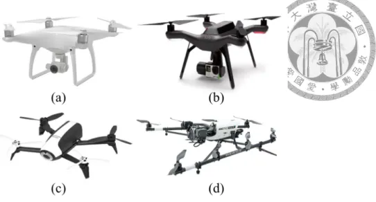
1.1 The state-of-the-art MAVs. (a) DJI Phantom 4. (b) 3DR Solo. (c) Parrot Bebop 2. (d) AscTec Falcon 8. . . 2 1.2 The visual and inertial sensors used in our experiments. (a) The used x-

IMU. (b) The RGB camera on Phantom 4. . . 4

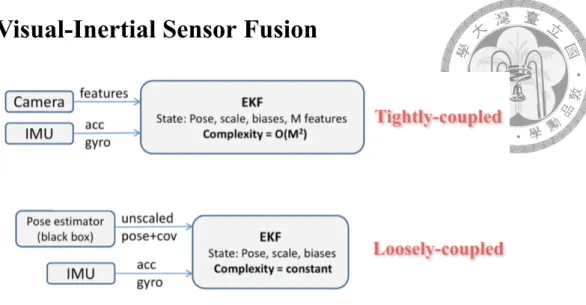
2.1 The differences between direct methods and feature-based methods. This figure is from [1]. . . 5 2.2 The differences between tightly-coupled methods and loosely-coupled meth-

ods. This figure is from [2]. . . 7

3.1 The overview of Model-Based Localization. . . 9 3.2 Overview over the complete LSD-SLAM algorithm. . . 10 3.3 Overview over the complete ORB-SLAM algorithm. This figure is from

their paper [3]. . . 12

4.1 Overview of the visual-inertial positioning framework in this paper. The blue blocks represent the measurements. . . 15 4.2 The Kalman filter steps in the sensor fusion framework. The red parts

are sensor readings (from the IMU for prediction or from another sensor for the update). The blue parts are the parts which change if the update sensor type changes. The black parts are the constant parts which stay analytically the same. . . 17

(8)

5.1 The Vicon Bonita motion capture system which offers the position ground truth in our indoor experiments. . . 18 5.2 The setup of our indoor experiments. . . 19 5.3 The visualized positioning results of the three methods in indoor experi-

ments. . . 20 5.4 The positioning results of Test 1 in outdoor experiments. On the right is

the experiment scene located in the CSIE Building in NTU. . . 21 5.5 The positioning results of Test 2 in outdoor experiments. On the right is

the experiment scene located in front of the Barry Lam Building in NTU. 21 5.6 Positioning results of LSD-SLAM and ORB-SLAM compared with the

ground truth in different movement speed. The mean errors (cm) are computed. . . 22 5.7 The relationship between different levels of blur and the positioning errors

of LSD-SLAM and ORB-SLAM. . . 23 5.8 Positioning results of LSD-SLAM and ORB-SLAM under different levels

of blur. . . 24 5.9 The performance of the three methods in different scenarios. . . 25 5.10 The framework in our experiment, where the visual result is simulated by

the Vicon measurement with noise. . . 26 5.11 The 3D visualized input measurement and the fusion result shown together. 26 5.12 The position measurements before and after sensor fusion in the three

axes. For each axis, the upper is the input measurement with σ = 0.1m Gaussian noise, and the lower is the fusion result. Both of them are compared with ground truth in red. . . 27

(9)

List of Tables

5.1 Positioning error (cm) of the three different methods in indoor experiments. 20 5.2 Positioning errors (cm) of LSD-SLAM and ORB-SLAM in different move-

ment speed. . . 23 5.3 Positioning errors (cm) before and after sensor fusion. . . 27

(10)

Chapter 1 Introduction

1.1 Motivation

With the development of technology, Micro Aerial Vehicles (MAVs) are widely used in industry and daily life. A MAV is a class of miniature Unmanned Aerial Vehicles (UAVs) that has a size restriction and is always autonomous. Development of MAV is driven by commercial, research, government, and military purposes. The small craft allows remote observation of hazardous environments inaccessible to ground vehicles. MAVs also have been built for hobby purposes, such as aerial robotics contests and aerial photography. One of the most representative MAV products in recent years is the Phantom 4 [4] developed by DJI, as shown in Figure 1.1 with other popular products. This kind of products is usually equipped with a camera and has been widely used in aerial cinematography and photography, so they can be also called flying cameras. To enable the flying cameras to navigate autonomously in different environments, accurate and robust ego-positioning is indispensable.

1.2 Positioning Techniques for Flying Cameras

Ego-positioning aims at locating an object in a coordinate system based on the sensors mounted on the object. For outdoor positioning, the Global Positioning System (GPS) is the most popular positioning technology in the past few decades. However, the precision

(11)

Figure 1.1: The state-of-the-art MAVs. (a) DJI Phantom 4. (b) 3DR Solo. (c) Parrot Bebop 2. (d) AscTec Falcon 8.

of GPS sensors is around 3 to 20 meters [5,6] and hard to meet the requirement in accurate navigation. Furthermore, existing GPS systems do not perform well in urban areas full of high rises and cannot work in indoor environments. Because of the drawbacks of existing GPS, other positioning methods more accurate and independent of external signals are needed. Laser scanners can achieve high accuracy, but the sensor suites are too bulky to be practical on flying cameras. From the trend in recent years, vision-based positioning is probably the most viable solution for flying cameras with very limited weight, since visual solutions only required to carry very lightweight, cheap cameras and are capable of running in real time.

1.3 Visual Positioning

Nowadays the vision-based positioning is well studied in the community and a variety of solutions are available, mostly known as Simultaneous Localization and Mapping (SLAM). In terms of different kinds of cameras, vision-based positioning can be divided into RGB-D, Stereo and Monocular. The RGB-D sensor consists of a RGB camera, an infrared (IR) camera and an IR projector. RGB-D cameras such as Microsoft Kinect [7]

provides both color images and dense depth maps at full video frame rate. This allows creating a new approach to visual positioning that combines the scale information of 3D

(12)

depth sensing with the strengths of visual features [8,9]. However, this kind of sensors cannot be used in outdoor environments and has great restrictions in the depth distance, so RGB-D cameras are not applicable for the positioning for flying cameras. A stereo camera is a type of camera with two or more lenses with a separate image sensor for each lens.

This allows the camera to simulate human binocular vision, and gives it the ability to per- ceive the depth in real scale from the images [10,11]. The fixed small baseline means the estimated distance will be less precise due to narrow triangulation, so the stereo cameras have bad performance in large-scale outdoor environments.

In [12,13] the authors reduced the sensor suite to one single camera, which is known as monocular visual odometry. One of the major benefits of monocular SLAM comes with the inherent scale-ambiguity, which allows to seamlessly switch between differently scaled environments, such as indoor environments and large-scale outdoor environments.

Scaled sensors on the other hand, such as depth or stereo cameras, have a limited range at which they provide reliable measurements and hence do not provide this flexibility.

Another advantage of monocular cameras is that it can be very low cost and has been widely equipped on existing MAVs. There is almost no demand to add additional sensors since most commercial MAVs are equipped with cameras as basic configuration. In recent years, many efforts have been made aiming to perform monocular visual SLAM in real time and the community launches a variety of visual positioning frameworks for different purposes [1,3,13–16]. In this paper, we evaluate the performance of the most representative state-of-the-art monocular methods and discuss on the pros and cons of them. We aim to find their most suitable application scenarios respectively and discuss the possible complementary combination in the future.

1.4 Inertial Sensor

Although monocular visual positioning is probably the most viable solution for flying cameras, there are still some limitations. Vision-only solutions rely heavily on the image quality and the number of feature points, so this kind of methods is easy to fail with serious blur or lack of features. Furthermore, the monocular solutions suffer from the lack of

(13)

(a) (b)

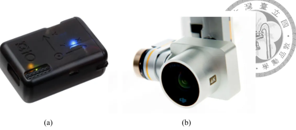
Figure 1.2: The visual and inertial sensors used in our experiments. (a) The used x-IMU.

(b) The RGB camera on Phantom 4.

metric scale. Considering these drawbacks, a well known direction is to fuse the Inertial Measurement Unit (IMU) with the vision result [2,17–19]. An inertial measurement unit (IMU) typically comprises three orthogonal accelerometers to measure the acceleration of the body, and also includes three orthogonal gyroscopes to measure the rate of change of the body’s orientation. Linear velocity and position, and angular position are obtained by integration or double integration. This is the principle behind inertial navigation systems (INS) which are used in aerospace and naval applications. An IMU is small in size, low cost and power efficient and thus is suitable for flying cameras. In this paper, we fuse the inertial data with the visual positioning result using a loosely-coupled method [20]. The used sensors are x-IMU [21] and the RGB camera mounted on the Phanthom 4, as shown in Figure 1.2.

(14)

Chapter 2 Related Works

2.1 Monocular Visual Positioning

For monocular SLAM, the early solutions are filter-based approaches [14,22,23], in which every frame is processed by the filter to jointly estimate the map points and the camera pose. It has the drawbacks of wasting computation in processing consecutive frames with little new information and the accumulation of linearization errors. The later proposed keyframe-based approaches [13] estimate the map using only selected frames, allowing to perform more costly but accurate bundle adjustment optimizations.

Figure 2.1: The differences between direct methods and feature-based methods. This figure is from [1].

(15)

Monocular SLAM approaches can be divided into two categories – direct and feature- based, as shown in Figure 2.1. Direct methods optimize the geometry directly on the image intensities, which enables using all information in the image, including e.g. edges –while feature-based approaches can only use small patches around corners. This leads to higher accuracy and more robustness in sparsely textured environments (e.g. indoors), and a much denser 3D reconstruction. In [15,24,25], accurate and fully dense depth maps are computed, which is computationally demanding and requires novel GPU to run in real time. In [26], a semi-dense depth filtering formulation was proposed which significantly reduces computational complexity, allowing real-time operation on a CPU and even on a modern smartphone [27]. In [1], the authors propose a Large-Scale Direct Monocular SLAM (LSD-SLAM) method, which not only locally tracks the motion of the camera, but also builds consistent, large-scale maps of the environment including loop-closures in real time. The benefits of direct method are higher accuracy and robustness in particular in environments with few features, and this method provides substantially more information about the geometry of the environment.

Feature-based methods performs feature extraction and matching before optimizations. The most representative feature-based SLAM system is probably Parallel Tracking and Mapping (PTAM) [13]. It was the first work to introduce the idea of splitting camera tracking and mapping in parallel threads, and demonstrated to be successful for real time augmented reality applications in small environments. PTAM has become a standard in monocular vision, and it has been adapted for MAVs navigation [28]. Recently an impres- sive real-time monocular SLAM systems called ORB-SLAM [3] that uses the efficient ORB feature has been presented. In this work, they implement a complete system that operates in real time with the capability of wide baseline loop closing and relocalization.

In addition to visual SLAM which performs mapping at the same time, there is an alternative to build the map or model previously, known as Model-Based Localization (MBL) [16]. This kind of approach applies to the ego-positioning in a known or repeatedly passed area.

(16)

2.2 Visual-Inertial Sensor Fusion

Figure 2.2: The differences between tightly-coupled methods and loosely-coupled methods. This figure is from [2].

The visual-inertial fusion approaches found in the literature can be divided into two categories: Tightly-coupled and loosely-coupled. Tightly-coupled approaches directly fuse the visual and inertial data, thus considering all correlations amongst them and achiev- ing higher precision. In [17], the authors propose an Extended Kalman Filter (EKF)- based real-time fusion using monocular vision, named Multi-state Constraint Kalman Fil- ter (MSCKF). This work performs with errors below 0.5 percent of the distance traveled.

In [29], a novel EKF-based algorithm is proposed, named MSCKF 2.0. The method described in [19] applies keyframe concept into nonlinear optimization by marginalization to achieve better accuracy.

Loosely-coupled systems in contrast process the IMU measurements and vision measurements separately, limiting computational complexity, seen as the simplest and most computationally efficient approach. Separately processing the two sources of information leads to a reduction in computational cost, and as a result loosely coupled methods are typically suited for systems with very limited resources, such as flying cameras [30]. Weiss et al. [2] propose an EKF-based algorithm that is independent of the underlying vision algorithm which estimates the camera poses. They later present a versatile framework to enable autonomous flights of a MAV in [20] by treating the visual part as a black box.

This method is suitable for us to implement on flying cameras since it is computationally efficient and can be easily used with different visual positioning algorithms.

(17)

Chapter 3 Visual Positioning for Flying Cameras

As described in the previous section, we choose three of the most representative state- of-the-art monocular solutions for experiment, which are MBL, ORB-SLAM and LSD- SLAM.

3.1 Model-Based Localization

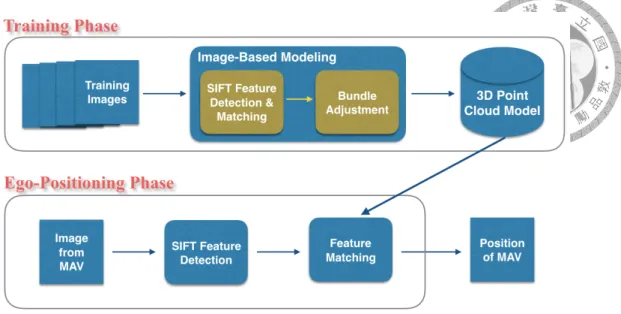
Model-based visual localization applies to the scenarios that we want to know our position in a known or repeatedly passed area. The major difference between MBL and SLAM methods is that MBL builds the global map or model previously before localization, while SLAM methods perform the localization and mapping simultaneously. The MBL method proposed by Chen et al. [16] consists of two phases – the training phase and the ego-positioning phase, as shown in Figure 3.1.

3.1.1 Training Phase

In the training phase, image-based modeling is performed, which aims to construct a 3D point cloud model from a number of input images. One of the well-known image-based modeling systems is the Photo Tourism method [1], which uses structure from motion to estimate camera poses as well as reconstruct 3D scene geometry from images simultaneously. Firstly, SIFT features are extracted upon each image in the image collection.

For every image pair, the feature point descriptors are matched with approximate nearest

(18)

Figure 3.1: The overview of Model-Based Localization.

neighbors, and the fundamental matrices of all pairs are estimated using RANSAC, sub- sequently. In the next step, an incremental Structure from Motion (SfM) method is used to avoid bad local minimal solutions and to reduce the computational load. It recovers camera parameters and 3D locations of feature points by minimizing the sum of distances between the projections of 3D feature points and their corresponding image features based on the following objective function:

mincj,Pi

∑n

i=1

∑m

j=1

v_ijd (Q(c_j, P_i), p_ij) , (3.1)

where c_jis the camera parameters of image j; m is the number of images; P_iis 3D coordi- nates of feature point i; n is the number of feature points; v_ij denotes the binary variables that equals 1 if point i is visible in image j and 0 otherwise; Q(c_j, P_i) projects the 3D point i onto the image j; p_ij is the corresponding image feature of i on j; and d(.) is the distance function. This objective function can be solved by using bundle adjustment, and a 3D point cloud model is built simultaneously. It includes the positions of 3D feature points and the corresponding SIFT feature descriptor list for each point.

(19)

3.1.2 Ego-Positioning Phase

In the ego-positioning phase, 2D-to-3D image matching and localization is performed, which aims to find the correspondences between 2D and 3D feature points and then compute the position of the 2D image in the 3D model. Given a test image, its SIFT features are firstly detected and the descriptors are computed at the same time. 2D-to-3D matching is referred to as finding the correspondence of the 2D points in the test image and the 3D points in the compressed model. Then, the camera position can be estimated based on the correspondence using the 6-point DLT algorithm with RANSAC.

3.2 LSD-SLAM

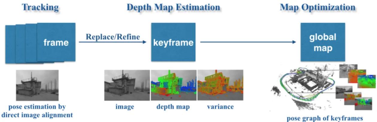
LSD-SLAM [1] is a novel, direct monocular SLAM method, which directly operates on image intensities both for tracking and mapping, instead of using feature points. The algorithm consists of three major components – tracking, depth map estimation and map optimization. The overview of the complete algorithm is shown in Figure 3.2.

Figure 3.2: Overview over the complete LSD-SLAM algorithm.

3.2.1 Tracking

The tracking component continuously tracks new frames with the current keyframe as reference. It estimates their rigid body pose ξ ∈ se(3) with respect to the current keyframe.

The pose of the previous frame is used as initialization. For pose estimation, direct image

(20)

alignment is performed using a novel method proposed in their paper, which directly uses image intensities instead of feature points.

3.2.2 Depth Map Estimation

The depth map estimation component uses tracked frames to either refine or replace the current keyframe. A frame is chosen to become a new keyframe once the camera has moved too far. Tracked frames that do not become a new keyframe are used to refine the depth map of the current keyframe. The map is refined by filtering over many per-pixel, small-baseline stereo comparisons as well as interleaved spatial regularization.

3.2.3 Map Optimization

Once a keyframe is replaced, it is incorporated into the global map which is a pose graph of keyframes by map optimization. In this component, a similarity transform ξ ∈ sim(3) to close-by existing keyframes is estimated using scale-aware, direct image align- ment to detect loop closures and scale-drift.

3.3 ORB-SLAM

ORB-SLAM [3] is the state-of-the-art feature-based SLAM method. It uses the ORB [31] (Oriented FAST and Rotated BRIEF) features which is extremely fast to compute and match. It is also invariant to rotation and scale in a certain range. Overview of the complete algorithm are shown in Figure 3.3. This feature-based SLAM system consists of three threads that run in parallel: tracking, local mapping and loop closing.

3.3.1 Tracking

The tracking thread performs image localization frame by frame and decides when to use the current frame as a new keyframe. It firstly uses a constant velocity motion model to roughly estimate the pose of a new frame and performs an initial matching with the previous frame, then it use a local map to project into the current frame and adjust the

(21)

Figure 3.3: Overview over the complete ORB-SLAM algorithm. This figure is from their paper [3].

camera pose by minimizing the reprojection error. After tracking on local map, the current frame is decided whether to be a new keyframe according to some thresholds.

3.3.2 Local Mapping

Local mapping is only performed on new keyframe K_i. At first the new keyframe is inserted into the global covisibility graph map and is used to update the nodes and edges in the covisibility graph. New map points are created by triangulating the ORB feature points. Then it performs a local bundle adjustment to optimize all the variables including the currently keyframe K_i, all the other keyframes connected to the current keyframe in the graph Kc, and all the map points that are seen by those keyframes. In order to maintain a condensed map and a compact reconstruction, redundant map points as well as keyframes are detected and culled in this thread.

(22)

3.3.3 Loop Closing

The loop closing thread uses the current keyframe K_ito detect loops and close them.

A bags of words place recognition module is embedded in the system, which consists of a visual vocabulary and a recognition database. It uses a pre-trained visual vocabulary to replace high dimensional ORB features in the loop detection for efficiency. If a loop is detected, it computes the 7-DoF similarity transformation from the current keyframe K_i to the corresponding loop keyframe K_l, which informs the accumulative error in the loop.

Then in the loop correction, the duplicated points in the map are fused and new edges are generated and inserted in the global map that attaches the loop closure. At last, a graph optimization is performed over an essential graph which is built and maintained by the system for efficiency to close the loop in real time.

(23)

Chapter 4 Visual-Inertial Sensor Fusion

4.1 Framework Overview

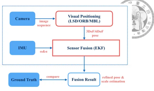
As discussed above, we advocate the EKF-based loosely-coupled sensor fusion described in [20]. Since IMU measurements and visual measurements are processed separately, we can divide the whole system into two independent modules – the visual positioning and the visual-inertial sensor fusion. Figure 4.1 shows the overview of the framework in this paper. For the visual positioning, we choose the most representative three state-of- the-art monocular solutions to evaluate and discuss on the pros and cons of each method, which are MBL, ORB-SLAM and LSD-SLAM. We aim to find their most suitable application scenarios respectively and discuss the possible complementary combination in the future. In the visual-inertial sensor fusion part, the fixed input is the IMU measurement and the changeable input is the visual measurement. The visual measurement can be the odometry result from any of the three above-mentioned methods, since we use the loosely-coupled method that treats the visual part as a black box. The output is the fusion result which can be compared with the ground truth.

4.2 Method

The loosely-coupled visual-inertial sensor fusion method proposed by Weiss et al. [20]

does not only estimate pose and velocity, but also estimate the scale of the position mea-

(24)

Figure 4.1: Overview of the visual-inertial positioning framework in this paper. The blue blocks represent the measurements.

surement and detect failures of the visual part. They verified the function of their method by fusing IMU data with PTAM visual measurement in their experiment [2]. As the visual framework is treated as a black box that has strong portability, we can use this method in our framework to fuse IMU data with the above-mentioned visual algorithms. This method uses an Extended Kalman Filter (EKF) framework, which generally consists of a prediction and an update step. Following gives an overview about the underlying structure of the EKF framework.

4.2.1 State Representation

The state of the filter is composed of the position of the IMU pⁱ_w in the inertial world frame, its velocity v_wⁱ and its attitude quaternion q_wⁱ describing a rotation from the inertial to the IMU frame. They add the gyro and acceleration biases b_ωand b_aas well as a possible measurement scale factor λ. The calibration states are the rotation from the IMU frame to the measurement sensor frame q^s_i and the distance between these two sensors p^s_i. The calibration states can be omitted and set to a calibrated constant making the filter more

(25)

robust. The state vector X:

X ={pⁱw

T vⁱ_w^T qⁱ_w^T b^T_w b^T_a λ p^s_i q_i^s} (4.1)

4.2.2 Prediction Step

IMU reading is used in the prediction step for state propagation, as the motion model in a basic Kalman Filter. The angular velocity ω and acceleration a readings from IMU are used to predict the system state by integration and double-integration. The following differential equations govern the state:

˙pⁱ_w = v_wⁱ (4.2)

˙vⁱ_w = C_(q^Ti

w)(a_m− ba− na)− g (4.3)

˙ q_wⁱ = 1

2Ω(ω_m− bω− nω)q_ωⁱ (4.4)

˙b_w = n_b_w ˙b_a = n_b_a ˙λ = 0 p˙^s_i = 0 q˙_i^s= 0 (4.5)

With g as the gravity vector in the world frame, Ω(ω) as the quaternion multiplication matrix of ω, and C_(q_wⁱ₎ as the IMU’s attitude in the world frame.

4.2.3 Update Step

Visual positioning result is used in the update step as the measurement in a basic Kalman Filter. For the position measurement z_p obtained from the visual algorithm, we have the following measurement model:

z_p = p^s_w = (pⁱ_w + C_(q^Ti

w)p^s_i)λ + n_p (4.6)

For the rotation measurement z_q obtained from the vision algorithm, we can model this as:

zq = q_w^s = q_i^s⊗ qⁱw (4.7)

(26)

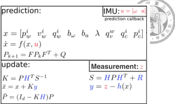
Figure 4.2: The Kalman filter steps in the sensor fusion framework. The red parts are sensor readings (from the IMU for prediction or from another sensor for the update). The blue parts are the parts which change if the update sensor type changes. The black parts are the constant parts which stay analytically the same.

Having known the measurement model, the state estimation can be updated according to the well known Kalman Filter procedure as shown in Figure 4.2. F and Q can be calculated according to [2]. In this method, the scale drift is handled by the scale estimate in real time and the failures of the vision part can be detected when there occurs an abrupt jump in the smooth drift estimation.

(27)

Chapter 5 Experiments

Figure 5.1: The Vicon Bonita motion capture system which offers the position ground truth in our indoor experiments.

In this section, we first evaluate the performance of the three chosen visual methods in five different scenarios – indoor, outdoor, rotation-only, fast-moving and blurry, aiming to find out the pros and cons of each method. In our experiments, video sequences from the onboard camera of Phantom 4 are used for test. The ground truth of each video sequence in our indoor experiments is measured using the Vicon motion capture system with four Bonita cameras [32]. In the experiments, the flying camera navigates under this system which consists of four optical capture cameras, as shown in Figure 5. The setup of the

(28)

flying camera in our indoor experiments is shown in Figure 5. Then we evaluate the sensor fusion performance by comparing the input measurement and the fusion result. In the simulation experiment，Vicon data is used to simulate the visual measurement.

Figure 5.2: The setup of our indoor experiments.

5.1 Evaluation for Different Visual Positioning Methods

To evaluate the performance of the LSD-SLAM, ORB-SLAM and MBL, several scenarios have been designed for test.

5.1.1 Indoor

To evaluate the performance for indoor positioning, we use two video sequences for test. In Test 1, the camera moves along a loop in the room facing the center of the circle, while in Test 2 it faces forward. The positioning result The visualized result is shown in Figure 5.3 where the red markers represent the positioning result at every keyframe and the blue ones represent the corresponding ground truth, the better the closer.

ORB-SLAM and MBL outperform LSD-SLAM in both Test 1 and Test 2, since we see the marker pairs match worse in the LSD-SLAM result than the other two methods.

Table 5.1 gives the quantitative comparison, which shows MBL is narrowly better than ORB-SLAM. Noticed that the performance of MBL depends on the training data. It may perform worse than ORB-SLAM with not enough training data.

(29)

Figure 5.3: The visualized positioning results of the three methods in indoor experiments.

Table 5.1: Positioning error (cm) of the three different methods in indoor experiments.

Test LSD-SLAM ORB-SLAM MBL

Mean Stdev. Mean Stdev. Mean Stdev.

#1 3.57 1.18 1.97 1.18 1.78 0.77

#2 4.46 2.13 2.23 1.06 2.09 1.14

5.1.2 Outdoor

Performance of large-scale outdoor positioning cannot be quantitatively evaluated, since we do not have Vicon as ground truth. Nevertheless, we can still evaluate the performance by analyzing a closed loop. We choose two scenes for experiment. The results are in Figure 5.4 and Figure 5.5. As shown in Figure 5.5, the flying camera takes a flight in front of the Barry Lam Building in NTU and finally stop at the starting point. The result of MBL can be approximately regarded as ground truth since this method processes each frame independently, which has no accumulative error. SLAM methods suffer from this kind of accumulative error, so in the results of LSD-SLAM and ORB-SLAM there are obvious drifts, although ORB-SLAM still outperforms LSD-SLAM. The obvious drifts occurs since there is a pure rotation movement during the flight, which will be discussed in the next paragraph.

(30)

Figure 5.4: The positioning results of Test 1 in outdoor experiments. On the right is the experiment scene located in the CSIE Building in NTU.

Figure 5.5: The positioning results of Test 2 in outdoor experiments. On the right is the experiment scene located in front of the Barry Lam Building in NTU.

(31)

5.1.3 Pure Rotation

Pure rotation means that there is only rotation and no translation between two consecu- tively tracked frames. It is especially common for flying cameras, because people usually make them hover in the air and only rotate the cameras for photography, which is uncommon for vehicles. In this case, the pose estimation between these two frames fails and the tracking is lost due to the lack of depth perception, as shown in outdoor experiment. Only MBL can survive this situation, since it does not track the current frame with respect to the previous frame but the pre-built model.

5.1.4 Fast-Moving

With the increase of the movement speed of the flying camera, the distance between two consecutive frames increases accordingly. We sample a testing video to simulate different speed, eliminating the influence of motion blur. The result is shown in Table 5.2 that the positioning error increases with the growth of speed until the tracking becomes completely lost. Noticed that the MBL is not in the experiment, because in MBL the tracking is irrelevant to other frames, the same reason with in the rotation-only situation.

Figure 5.6: Positioning results of LSD-SLAM and ORB-SLAM compared with the ground truth in different movement speed. The mean errors (cm) are computed.

(32)

Table 5.2: Positioning errors (cm) of LSD-SLAM and ORB-SLAM in different movement speed.

Speed LSD-SLAM ORB-SLAM

Mean Stdev. Mean Stdev.

x1 5.50 2.71 1.56 0.63

x2 6.74 3.04 3.21 1.49

x3 7.92 3.82 3.78 1.68

5.1.5 Blurry

Motion blur is an always existent issue for vision-based method. We design this experiment to compare the difference between direct method and feature-based method in blurry situations. In this experiment, we manually add motion blur from 5 to 35 pixels onto the test video sequence. Experiment result in Figure 5.7 shows that within certain range of blur, the feature-based method (OBR-SLAM) has much better accuracy. How- ever, when the blur becomes large (over 20 pixels in the experiment), the feature-based method suddenly turns into the non-initial mode, which means it cannot match enough features for initialization. In contrast the direct method (LSD-SLAM) is very robust with the error increasing slowly, since this kind of methods does not need to extract features and can avoid the corresponding artifacts.

Figure 5.7: The relationship between different levels of blur and the positioning errors of LSD-SLAM and ORB-SLAM.

(33)

Figure 5.8: Positioning results of LSD-SLAM and ORB-SLAM under different levels of blur.

5.1.6 Comparison

We arrange the results of the above experiments and discussions into the table in Fig- ure 5.9. According to the experiment results, LSD-SLAM and ORB-SLAM have similar pros and cons since they both are SLAM methods. LSD-SLAM is better during blurry or featureless cases while ORB-SLAM has better accuracy in common cases, which shows the difference between direct methods and feature-based methods. MBL is different from other methods since it has a pre-built model, tracking each frame independently. It has advantages of not being affected by pure rotation and accumulative error, and it provides global positioning which is useful when there are more than one flying camera.

(34)

Figure 5.9: The performance of the three methods in different scenarios.

5.2 Evaluation for Sensor Fusion Results

Sensor fusion is used to make up for the limitations of visual positioning. Noticed that the visual positioning methods mentioned above are accurate, so it is hard to achieve significantly better accuracy by loosely-coupled sensor fusion methods. However, we can still verify the function of this sensor fusion method by designing a bad case. In this experiment, we add a Gaussian noise onto the Vicon measurement to simulate bad visual positioning result, and then fuse it with IMU readings. Figure 5.10 shows the framework in our simulation experiment.

In the experiment, the used inertial sensor is x-IMU [21]. The IMU moves under the Vicon system and the angular velocity ω and acceleration a readings are used to predict the system state in the EKF-based framework. As discussed before, the visual part is considered as a black box, so it is feasible to use Vicon data in this part as measurement.

We add σ = 0.1m Gaussian noise onto Vicon measurement to simulate bad vision cases.

The mean error in 3D space is 16.01cm after adding the noise. Fusion result is shown below. The 3D visualized input measurement and the fusion result are shown together in Figure 5.11. Figure 5.12 shows the input and the output in the three axes in the sensor fusion experiment, from which we see the noise has been reduced significantly and the curve is much more smooth. Table 5.3 shows the quantitative results, from which the 3D positioning error has been reduced to 8.68cm from 16.01cm.

(35)

Figure 5.10: The framework in our experiment, where the visual result is simulated by the Vicon measurement with noise.

Figure 5.11: The 3D visualized input measurement and the fusion result shown together.

(36)

Table 5.3: Positioning errors (cm) before and after sensor fusion.

Axis Measurement Fusion Result Mean Stdev. Mean Stdev.

x 8.23 6.09 4.00 2.93

y 7.79 5.77 4.21 3.22

z 8.09 6.05 4.67 3.34

3D 16.01 6.67 8.68 3.36

Figure 5.12: The position measurements before and after sensor fusion in the three axes.

For each axis, the upper is the input measurement with σ = 0.1m Gaussian noise, and the lower is the fusion result. Both of them are compared with ground truth in red.

(37)

Chapter 6 Conclusion and Future Works

6.1 Conclusion and Future Work

In this paper, we have evaluated the three different visual positioning methods in many scenarios. LSD-SLAM is less accurate but more robust in featureless and blurry cases.

It uses the most information and its dense reconstruction is useful for other tasks than just localization. ORB-SLAM achieves impressively high precision most of the time but still has the nature defects of both SLAM methods and feature-based methods. MBL proves to be the most robust method in monocular positioning by localizing each frame independently. However, it cannot be used in unknown environment since the model need to be built previously and the positioning performance depends on the training images. To make up for the limitations of vision, we use an IMU to aid visual positioning by sensor fusion. The experiment shows that it helps reduce the positioning error in bad cases and the metric scale which is not observable in monocular positioning can be estimated.

We find that the pure rotation situation is an important issue in ego-positioning for flying cameras, which is uncommon in positioning for vehicles. While the SLAM methods all suffer from this situation, MBL shows its robustness. It is a valuable future topic to use them for complementary combination. ORB-SLAM is used for general tracking and helps update the model in unknown area. LSD-SLAM can be combined as a spare module for featureless or blurry cases. MBL is used to correct the accumulative drift and handle the pure rotation cases, and it is also used for global positioning.

(38)

Bibliography

[1] Jakob Engel, Thomas Schóps, and Daniel Cremers. Lsd-slam: Large-scale direct monocular slam. In European Conference on Computer Vision, pages 834–849.

Springer, 2014.

[2] Stephan Weiss and Roland Siegwart. Real-time metric state estimation for modular vision-inertial systems. In Robotics and Automation (ICRA), 2011 IEEE Interna- tional Conference on, pages 4531–4537. IEEE, 2011.

[3] Raul Mur-Artal, JMM Montiel, and Juan D Tardós. Orb-slam: a versatile and ac- curate monocular slam system. IEEE Transactions on Robotics, 31(5):1147–1163, 2015.

[4] DJI. Dji phantom series. http://www.dji.com/cn/products/phantom.

[5] Ted Driver. Long-term prediction of gps accuracy: Understanding the fundamentals.

In ION GNSS, 2007.

[6] Marko Modsching, Ronny Kramer, and Klaus ten Hagen. Field trial on gps accuracy in a medium size city: The influence of built-up. In 3Rd workshop on positioning, navigation and communication, pages 209–218, 2006.

[7] Microsoft. Microsoft kinect. https://developer.microsoft.com/en- us/windows/kinect.

[8] Richard A Newcombe, Shahram Izadi, Otmar Hilliges, David Molyneaux, David Kim, Andrew J Davison, Pushmeet Kohi, Jamie Shotton, Steve Hodges, and Andrew Fitzgibbon. Kinectfusion: Real-time dense surface mapping and tracking. In Mixed

(39)

and augmented reality (ISMAR), 2011 10th IEEE international symposium on, pages 127–136. IEEE, 2011.

[9] Thomas Whelan, Stefan Leutenegger, Renato F Salas-Moreno, Ben Glocker, and Andrew J Davison. Elasticfusion: Dense slam without a pose graph. Proc. Robotics:

Science and Systems, Rome, Italy, 2015.

[10] Andrew Howard. Real-time stereo visual odometry for autonomous ground vehi- cles. In 2008 IEEE/RSJ International Conference on Intelligent Robots and Systems, pages 3946–3952. IEEE, 2008.

[11] David Schleicher, Luis M Bergasa, Manuel Ocaña, Rafael Barea, and Elena López.

Real-time hierarchical stereo visual slam in large-scale environments. Robotics and Autonomous Systems, 58(8):991–1002, 2010.

[12] Andrew J Davison. Real-time simultaneous localisation and mapping with a single camera. In Computer Vision, 2003. Proceedings. Ninth IEEE International Confer- ence on, pages 1403–1410. IEEE, 2003.

[13] Georg Klein and David Murray. Parallel tracking and mapping for small ar workspaces. In Mixed and Augmented Reality, 2007. ISMAR 2007. 6th IEEE and ACM International Symposium on, pages 225–234. IEEE, 2007.

[14] Andrew J Davison, Ian D Reid, Nicholas D Molton, and Olivier Stasse. Monoslam:

Real-time single camera slam. IEEE transactions on pattern analysis and machine intelligence, 29(6):1052–1067, 2007.

[15] Richard A Newcombe, Steven J Lovegrove, and Andrew J Davison. Dtam: Dense tracking and mapping in real-time. In 2011 international conference on computer vision, pages 2320–2327. IEEE, 2011.

[16] Kuan-Wen Chen, Chun-Hsin Wang, Xiao Wei, Qiao Liang, Chu-Song Chen, Ming- Hsuan Yang, and Yi-Ping Hung. Vision-based positioning for internet-of-vehicles.

IEEE Transactions on Intelligent Transportation Systems, 2016.

(40)

[17] Anastasios I Mourikis and Stergios I Roumeliotis. A multi-state constraint kalman filter for vision-aided inertial navigation. In Proceedings 2007 IEEE International Conference on Robotics and Automation, pages 3565–3572. IEEE, 2007.

[18] Jonathan Kelly and Gaurav S Sukhatme. Visual-inertial simultaneous localization, mapping and sensor-to-sensor self-calibration. In Computational Intelligence in Robotics and Automation (CIRA), 2009 IEEE International Symposium on, pages 360–368. IEEE, 2009.

[19] Stefan Leutenegger, Simon Lynen, Michael Bosse, Roland Siegwart, and Paul Fur- gale. Keyframe-based visual–inertial odometry using nonlinear optimization. The International Journal of Robotics Research, 34(3):314–334, 2015.

[20] Stephan Weiss, Markus W Achtelik, Margarita Chli, and Roland Siegwart. Versatile distributed pose estimation and sensor self-calibration for an autonomous mav. In Robotics and Automation (ICRA), 2012 IEEE International Conference on, pages 31–38. IEEE, 2012.

[21] x-io Technologies. x-imu. http://www.x-io.co.uk/products/x-imu/.

[22] Javier Civera, Andrew J Davison, and JM Martinez Montiel. Inverse depth parametrization for monocular slam. IEEE transactions on robotics, 24(5):932–945, 2008.

[23] Ethan Eade and Tom Drummond. Scalable monocular slam. In 2006 IEEE Com- puter Society Conference on Computer Vision and Pattern Recognition (CVPR’06), volume 1, pages 469–476. IEEE, 2006.

[24] Jan Stúhmer, Stefan Gumhold, and Daniel Cremers. Real-time dense geometry from a handheld camera. In Joint Pattern Recognition Symposium, pages 11–20. Springer, 2010.

[25] Matia Pizzoli, Christian Forster, and Davide Scaramuzza. Remode: Probabilistic, monocular dense reconstruction in real time. In 2014 IEEE International Conference on Robotics and Automation (ICRA), pages 2609–2616. IEEE, 2014.

(41)

[26] Jakob Engel, Jurgen Sturm, and Daniel Cremers. Semi-dense visual odometry for a monocular camera. In Proceedings of the IEEE international conference on com- puter vision, pages 1449–1456, 2013.

[27] Thomas Schöps, Jakob Engel, and Daniel Cremers. Semi-dense visual odometry for ar on a smartphone. In Mixed and Augmented Reality (ISMAR), 2014 IEEE Interna- tional Symposium on, pages 145–150. IEEE, 2014.

[28] Jakob Engel, Júrgen Sturm, and Daniel Cremers. Scale-aware navigation of a low- cost quadrocopter with a monocular camera. Robotics and Autonomous Systems, 62(11):1646–1656, 2014.

[29] Mingyang Li and Anastasios I Mourikis. High-precision, consistent ekf-based visual–inertial odometry. The International Journal of Robotics Research, 32(6):

690–711, 2013.

[30] Roland Brockers, Sara Susca, David Zhu, and Larry Matthies. Fully self-contained vision-aided navigation and landing of a micro air vehicle independent from exter- nal sensor inputs. In SPIE Defense, Security, and Sensing, pages 83870Q–83870Q.

International Society for Optics and Photonics, 2012.

[31] Ethan Rublee, Vincent Rabaud, Kurt Konolige, and Gary Bradski. Orb: An efficient alternative to sift or surf. In 2011 International conference on computer vision, pages 2564–2571. IEEE, 2011.

[32] Vicon. Vicon bonita. http://www.vicon.com/products/camera- systems/bonita.