歐洲金融機構營運風險與名譽損失

國立臺灣大學管理學院財務金融學系 碩士論文

Department of Finance College of Management National Taiwan University

Master Thesis

歐洲金融機構營運風險與名譽損失 Operational Risk and Reputation Loss in

European Financial Industry

陳建豪 Chien-Hao Chen

指導教授：何耕宇 博士 Advisor: Keng-Yu Ho, Ph.D.

中華民國 100 年 6 月

June, 2011

i

誌謝

研究所的生活很快地就要進入尾聲了，也終於到了期盼已久的寫誌謝文這一 刻了。這兩年在台大的校園學到很多，也成長很多，大學理工科系畢業的我，起 初不是很能適應競爭如此激烈的財金所，隨著博學多聞的師長帶領以及全台灣最 優秀的同儕們之間的相互扶持，我也總算走到研究所的最後這一刻了，心裡有很 多感觸，有很多人要感謝，無奈誌謝文只能寫短短的一頁，不然我打算寫一本書 來回憶、來誌謝，可惜！可惜！我們，長話短說吧！

這篇論文的完成，首先必須要感謝我的指導教授何老師，整個撰寫論文的過 程，老師總是非常細心且有耐心地給予幫助與指教，讓我有辦法在期限內完成這 篇論文，博士班的柏欣學長在程式碼的方面給了我很大的建議與幫助，在此感謝。

非常要好的朋友同時也是同門的小慧、若懷、小奚，有妳們的一起的奮鬥以及玩 樂真的是碩班最珍貴的回憶，還有很多要好的朋友，延瑋、怡婷、容嘉、凱銘、

定庭，謝謝你們時常在我的生活上給予照顧與關懷。

我的爸爸、媽媽、姊姊，是我一生中最重要的人，有您們的陪伴與關心是我 在往後的人生繼續成長向上的最佳動力，謝謝您們給我的一切，我會好好珍惜，

謹以此篇論文獻給我最愛的家人。

建豪 100/07 筆於台大

ii

Abstract

In this paper we focus on huge operational loss events in European financial companies in the past 20 years. The reputation loss is our main focus. We collect the operational loss companies’ stock price and calculate the difference between market value loss and announced loss to represent the reputation loss when the company have operational loss event. We separate our sample into two groups by year and compare short-term and long-term performance of these two groups. We find that the companies suffer more reputation loss when they have operational loss after year 2000 in both short run and long run. We also compare the UK financial companies’ operational loss events with other European financial companies’, and we find UK financial companies suffer more reputation loss when they have operational loss.

Index Terms — Operational Risk, Reputation Loss, European Financial Industry

iii

中文摘要

在這篇論文裡，我們研究歐洲的金融機構在過去 20 年發生大筆金額的營運損 失事件。名譽損失是我們主要探討的議題。我們針對這些營運損失的事件進行事 件研究法，我們收集公司宣告營運損失當下的股價資料，進而計算出公司因為營 運損失所造成的市值減少。市值的減少與公司宣告事件損失的金額並不會相同，

這兩者的差距我們便定義為名譽損失。我們把收集到的樣本以西元 2000 年作為一 個分界，我們的結果顯示西元 2000 年以後發生營運損失的公司，承受了較大的名 譽損失。同時我們的結果也顯示出這些發生營運損失的公司在長期股價表現較差。

在我們所有研究的樣本中，英國的金融機構發生的營運損失事件占了 40%以上，因 此我們將英國的金融機構與歐洲其他的金融機構做了比較，我們發現英國的金融 機構在發生營運損失事件後所承受的名譽損失大於其他的歐洲金融機構。

關鍵字：營運風險，名譽損失，歐洲金融機構

iv

Table of Contents

口試委員會審定書 ... #

誌謝 ... i

Abstract... ii

中文摘要 ... iii

1. Introduction ...1

2. Literature Review ...3

3. Data and Event Study Methodology ...5

3.1. Sample selection and data resource ...5

3.2. Methodology...7

3.2.1. Event study methodology in the short-term ...7

3.2.2. Event study methodology in long-term ...9

3.2.3. Regression model ...10

4. Empirical Result ... 11

4.1. Descriptive results ... 11

4.2. Event study result in the short-term ...12

4.2.1. Short-term regression result ...14

4.3. Event study result in the long-term ...15

4.3.1. Long-term regression result ...16

5. Conclusion ...17

References ...19

v

List of Tables and Figures

Table 1: Events’ loss amount and the number of observations ...22

Table 2: Operational risk loss event types ...23

Table 3: The test statistic for CAR and CAR(Rep) ...24

Table 4: The test statistic for CAR and CAR(Rep) in sub-sample grouped by year ...25

Table 5: The test statistic for CAR and CAR(Rep) in sub-sample grouped by country ..26

Table 6: Regression result: Dependent variable is CAR(Rep) ...27

Table 7: Regression result: Dependent variable is CAR ...28

Table 8: The test statistic for BHAR on three different periods ...29

Table 9: The test statistic for BHAR in sub-sample grouped by year ...30

Table 10: The test statistic for BHAR in sub-sample grouped by country ...31

Table 11: Regression result: Dependent variable is BHAR% ...32

Figure 1: CAR and CAR(Rep) : All-sample: ...33

Figure 2: CAR and CAR(Rep) : Events happen before year 2000 ...34

Figure 3: CAR and CAR(Rep) : Events happen after year 2000 ...35

Figure 4: CAR and CAR(Rep) : Event firms belong to UK. ...36

Figure 5: CAR and CAR(Rep) : Event firms belong to other European countries ...37

1

1. Introduction

The operational loss events caused by financial firms attract more attention in recent years. Financial industry is an industry which is highly regulated, but the operational loss events happen frequently. From Basel Committee, 2006, it indicate that Operational risk is the risk of loss resulting from inadequate or failed internal processes, people and systems, or from external events. There are more and more studies in this field. We collect operational loss events happen in European financial companies, and use these companies’ stock price to do event study. Our result shows the performance of the operational loss firm is poor during the announcement date.

The most interesting thing we would like to know is how the market and the investor evaluate these operational loss companies’ reputation. Reputation risk is an abstract concept, and the Board of Governors of Federal Reserve System (2004) makes a definition on it: Reputation risk is the potential that negatively publicity regarding an institution’s business practices, whether true or not, will cause a decline in the customer base, costly litigation, or revenue reductions. In this paper we calculate the difference between market value loss and announced loss to represent the reputation loss when the companies have operational loss events.

Previous literature use different methodologies to describe the reputation loss. No

2

matter how they change the formula, the basic parts to evaluate the reputation are the loss value of the company and the loss amount they announced or reported by press.

Their result shows the operational loss event damage the firm’s reputation. So they start to focus on difference reputation damage between different event types, and compare the cumulative abnormal return on different event dates like settlement date, recognition date, and announcement date.

In this paper we combine their method to calculate reputation loss, and we intend to make some different analysis. When we deal with our database and these operational loss firms’ reputation loss, we find that the reputation loss have more proportion in the market value loss in recent years. So we separate our samples into two groups by the events’ announcement date. One group is the events’ announcement dates happen before year 2000, another is the events’ announcement dates happen after year 2000. Our result shows the companies suffer more reputation loss when they have operational loss after year 2000. Due to our UK-company samples are exceed 40% in our all samples, we try to find the difference between UK-company samples and other European-company samples.

Previous studies focus on event study method, and they calculate the operational loss events’ cumulate abnormal return in event period to do analysis. These event studies’ event periods are short-term like one week trading-day before or after event

3

date. In this paper we collect these companies’ stock price after the event date at least one year to do the long-term performance analysis, and we find that the operational loss companies have worse return in the long-term.

The remained of this paper is organized as follow: In Section 2 we review the recent literature. In Section 3 we describe our database and the event study methodology.

We report our statistic result and regression result in Section 4. Finally, in Section 5 we have some conclusions.

2. Literature Review

De Fontnouvelle, Jordan, Rosengren, and DeJesus-Rueff (2003) they qualify operational risk and provide guidance to managers and regulators about the magnitude of operational risk capital in the banking industry. They find that operational loss is an important source of risk for large, internationally active banks. They also find that the capital charge for operational risk often exceed the charge for market risk.

Murphy, Shrieves, and Tibbs (2004) examine the market impact of allegation of firms’ misconduct such as anti-trust violations, bribery, copyright infringements, or accounting fraud. They find that the losses in wealth associated with allegations of fraud are substantially larger than those in the other categories examined. They also find that firm size is negatively related to the percentage loss in firm market value. They explain

4

this result by economy of scale effect and reputation effect. In economy of scale effect, if acts of misconduct impose fixed costs on the company, then percentage losses is smaller for the larger company. With the reputation effect, larger company with better brand name may more easily counter the reputational damage.

Perry and de Fontnouvelle (2005) assess the market reaction to operational loss announcement. They find that market values fall one-for-one with losses caused by external events, and fall by over twice the loss percentage when the loss is due to internal fraud. They also find the market reaction to internal fraud losses is worse when the company with strong shareholder rights.

Cummins, Lewis, and Wei (2006) conduct an event study on market value of operational loss events for US banks and insurance companies. They find that the market value respond negatively to operational loss announcements especially in the insurance companies. They propose three explanations about this result: (1) Insurance companies are slow to respond to operational risk while banks have begun to consider this risk. (2) Insurance companies are less protected than banks. (3) Insurers tend to be more highly capitalized than banks. They also find a positive relationship between losses and Tobin’s Q, it means operational loss events have a large impact for forms with better growth opportunity.

Gillet, Hubner, and Plunus (2010) examine the reputation impact on market returns

5

of operational events affecting US and European financial companies. They intend to isolate the pure reputation effect of the operational loss on market value by accounting the difference between market value and the loss amount. They focus on three event date: First press cutting date, Recognition Date, Settlement Date, and find that negative CAR around both press date and the recognition date. They also find that the market overreaction to loss events when the loss amount is unknown. They interpret this phenomenon as a consequence of asymmetric information on the financial industry, leading to an adverse selection type of behavior.

In this paper, we combine pervious papers’ methodology to calculate the reputation loss caused by operational loss, and we hypothesize these European financial companies have reputation loss when they have huge operational loss.

3. Data and Event Study Methodology

3.1. Sample selection and data resource

The data analyzed in this study are from First database, a data set provides by the Fitch Group. This database provides case studies analyzing operational risk loss events and descriptive information on the events. The events on this database all have the loss exceed $1 million. We focus on European financial companies and select 7 countries:

United Kingdom, France, Germany, Italy, Spain, Switzerland, and Netherland for our

6

analysis. There are too many events in our database, so we have to set some criteria to filter the database. All the operational loss events in First database are grouped by country. Some events happen in our targeted countries, but the firms are branch of other country’s companies and we delete these samples. We set a criterion that the loss amount must exceed $3 million. The reason for focusing on the large losses is that smaller loss is less likely to have influence on the stock price and less likely to be reported. Daily stock price and index come from Thomson Financial DataStream for the use of event study. After combining these two databases, we get 101 samples for our event study. We have to collect the market value of the company on the event date and the loss amount of the events for the reason to calculate the CAR(Rep) that represent the reputation loss. There are some missing data in loss amount or market value, so we have 79 samples in our final analysis. We also intend to calculate the buy-and-hold period abnormal return (BHAR) of every event, and we set the holding period is 1-year, 2-year 3-year after the event date. We collect the monthly stock return after event date and the corresponding market index. Some events happen after year 2008, so we can’t get enough stock price information to calculate these events’ two-year and three-year BHAR. We have 101 samples in one-year BHAR, 98 samples in two-year BHAR and 87 samples in three-year BHAR.

There are some dates about one event in our database: event start date, event end

7

date, settlement date, recognition date and announcement date. We focus on the investor’s response to the press news release in this paper, so we have to collect the announcement date which is available through the source of First database. There are many press news about one operational loss event in the source column. We manually collect these announcement date of each press news and choose the first announcement date as our announcement date of each event.

First database provides some data like the event company’s employees, total assets, total equity, total deposits, and total revenue that seems we can use in our regression model, however we find these data can’t be used in our study. First database provides these data base on the scaling date, and they are useless when we intend to have analysis according to announcement date. So we collect some independent variable like price to book ratio, market value, the number of employee, and return on asset from DataStream.

These data we collect from DataStream base on announcement date which we choose from press news, and it makes sense in our study.

3.2. Methodology

3.2.1. Event study methodology in the short-term

We want to analyze the stock price reaction to operational loss announcement in the short-term. Because we intend to know the market reaction on the announced news,

8

the announcement date is exactly the event date. We set an estimated period to predict the operational loss firm’s return during event period. This estimated period is 250-trading-day and 30-trading-day before the announcement date. We collect operational loss firms’ stock price and calculate their daily return. We use the corresponding market index to represent the market return. Model 1 is estimated using OLS regression over the estimated period. We set different event windows for analysis:

(-20,20), (-10,10), (-5,5), (0,1), (0,5), (0,10), (0,20). The event window (-20,20) means 20-trading-day before announcement date and 20-trading-day after announcement date.

We also have the real stock return and the market return during these periods. By using the α and β we get from model (1) and the market return we collect, we can get the firm’s expected return during the event period as model (2). The difference between the firm’s real return and the expected return is abnormal return (AR) as model (3).

R

_i =α β_i+ _i

R

_m+ε _i (1) ˆ_i = ˆ_i+ ˆ_{i m}

R

α β

R

(2)

= − ˆ

i i i

AR R R

(3) We adjust the abnormal return by considering loss amount and market value to get the AR(Rep) as model (4). We aggregate the AR from N-trading-day before announcement date to M-trading-day after announcement date to get the cumulative abnormal return (CAR) in window (-N, +M) as model (5). The reputation effect

9

happens after the announcement, so we aggregate the AR(Rep) from announcement date to M-trading-day after announcement date to get CAR(Rep) in window (0,+M) as model (6).

AR(Re p )

_i =

AR

_i+

| Loss _ amount / Market _ value |

_{i i}

(4)

2

1 2 1

[ , ] =

∑

^t

i t t t i

CAR AR

(5)

=

∑

²

2

t

i [ 0 ,t ] 0 i

CAR(Re p ) AR(Re p )

(6)

3.2.2. Event study methodology in long-term

In the meantime, we also intend to know the long-term performance of these companies’ stock price. We collect these companies’ monthly return in one-year, two-year, and three-year after the announcement date. We compare these stocks’ return with the market index to get the buy-and-hold abnormal return (BHAR). We use model (7) to get R , n-year return of i company. ⁿ_i R_i,1 is i company’s first month return. Rⁿ_m in model (8) is the market index’s n-year return. In model (9), we can get n-year BHAR,

n=1, 2, 3.

n 1/ 12 n

i i ,1 i ,2 i ,12 n

R =[( 1+R )( 1+R )...( 1+R )] (7) R_mⁿ =[( 1 R+ _{m ,1})( 1 R+ _{m ,2})...( 1 R+ _{m ,12n})]^{1/ 12n} (8) BHAR_iⁿ =R_iⁿ−R_mⁿ (9)

10

3.2.3. Regression model

In our short-term regression model, we list 7 independent variables: UK, Year 2000, Internal, PTBV, MV, Employee, and ROA. The dependent variable is CAR(Rep)% as model (10). We also have another regression model which the dependent variable is CAR% and we add one more independent variable: Loss_amount as model (11). In the long-term regression model, we list 8 independent variables: UK, Year 2000, Internal, PTBV, MV, Employee, ROA, and Loss_amount. The dependent variable is BHAR% as model (12). UK is a dummy variable, UK=1 if the company belongs to UK, Year 2000 is a dummy variable, Year 2000=1 if the event happens after year 2000, Internal is a dummy variable, Internal =1 if the event type is internal fraud, PTBV is the price-to-book ratio of company on the announcement date, MV is the market value of company on the announcement date, Employee is the number of employees of company on the announcement date, ROA is return on asset of the company on the announcement date, Loss_amount is the operational loss amount the company announced, C is

constant.

= + ₁ + ₂ + ₃ + ₄ + ₅

CAR(Re p ) C

β

UK

β

Year2000

β

Internal

β

PTBV

β

MV

+

β

₆

Employee

+

β

₇

ROA

(10)

= + ₁ + ₂ + ₃ + ₄ + ₅

CAR C

β

UK

β

Year2000

β

Internal

β

PTBV

β

MV

+β₆

Employee

+β₇

ROA

+β₈

Loss amount _

(11)

11

= + ₁ + ₂ + ₃ + ₄ + ₅

BHAR C

β

UK

β

Year2000

β

Internal

β

PTBV

β

MV

+β₆

Employee

+β₇

ROA

+β₈

Loss amount _

(12)

4. Empirical Result

4.1. Descriptive results

Table 1 shows the events’ loss amount and the number of observations from year 1990 to year 2010 in our targeted countries and their corresponding market index. In the previous literatures, they set European firms as one group, and their corresponding index is only FTSE 100 no matter the firm belongs to United Kingdom or not. In order to have precise result we use the market index, which the firm belongs to, to do the event study. There are 101 samples in our targeted countries during year 1990 to year 2010 and concentrate on 25 financial companies. We double check these events are independent on each other. The highest loss amount is $17518 million and the event company is Lloyds Banking Group. Our samples’ operational loss amount is at least $3 million because smaller loss is less likely to have influence on the stock price.

Table 2 shows the operational risk loss event types which grouped by Basel Committee. Our samples concentrate on three event types: External fraud, Internal fraud, and Clients Products and Business Practices. In our 101 operational loss events, 20 events are caused by External fraud, 20 events are caused by Internal fraud, and 38

12

events are unintentional or negligent failure to meet a professional obligation to specific clients.

4.2. Event study result in the short-term

Figure 1 shows the development of CAR’s mean from 20-trading-day before the announcement date to 20-trading-day after the announcement date. The dashed line illustrates the reputation effect, as the values of the operational loss amount divided by the market value of the company are added at date 0. We can see clearly both the CAR and CAR(Rep) go down during the announcement date . In the all sample result, the mean of CAR goes down to -4% in 40 trading days. We use CAR(Rep) to represent the firm’s reputation loss, and our CAR(Rep) goes down to -2% from announcement date to 20-trading-day after announcement date. When we draw this figure, we delete 22 samples that have CAR but have no CAR(Rep).

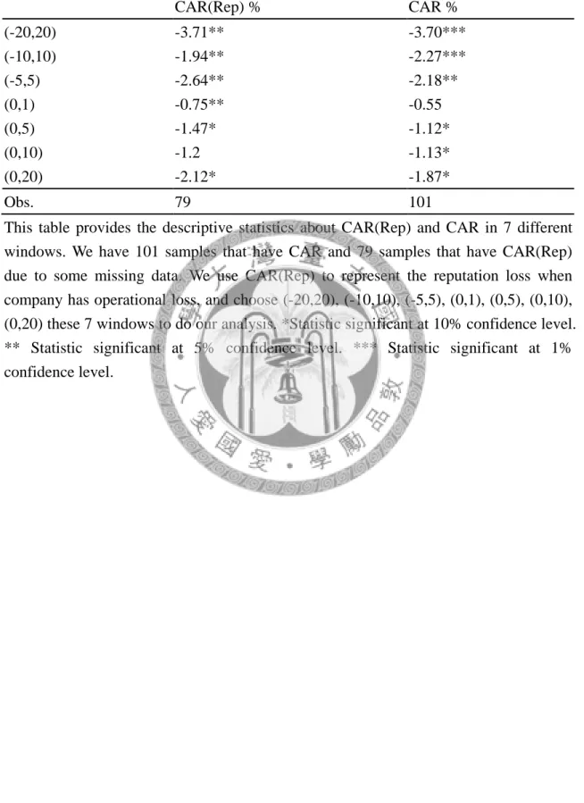
Table 3 shows the test statistic for CAR and CAR(Rep) in 7 different windows. We have 101 observations on CAR and 79 observations on CAR(Rep). Due to some missing data on loss amount and market value, we lose 22 observations on CAR(Rep).

We can see clearly both the CAR and CAR(Rep) are significant negative under different windows especially the CAR in the window (-20, 20) and (-10, 10). This result consists with our hypothesis that these European financial companies have reputation loss when

13

they have huge operational loss.

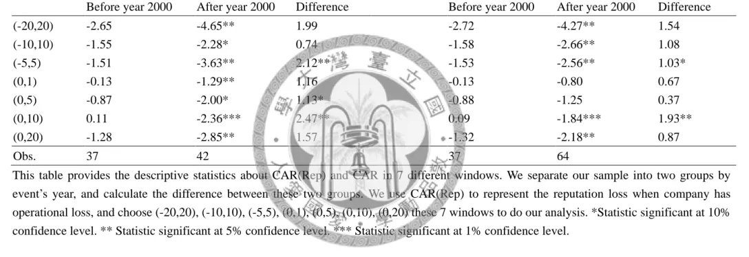
We separate our samples into two groups, one is the events happen before year 2000 another is the events happen after year 2000. We calculate the CAR(Rep) and CAR of these different windows. From Table 4 we can see the events happen after year 2000, their CAR(Rep) are significant negative. The events happen before year 2000 have negative CAR(Rep)s but the values are not significant in any window. In Figure 2 we show the short-term performance which the events happen before year 2000. There are something strange in Figure 2 that the CAR(Rep) during (8,13) is positive however it is not significant. We think that the investors in the market don’t think operational loss is a big mistake and think it is usual in the past. In Figure 3 we show the short-term performance which the events happen after year 2000. From Table 4, Figure 2, and Figure 3 we interpret that with the progress of internal control system, the investor on the market have stricter attitude toward operational loss events. We have a short conclusion that companies may loss more reputation when they get operational lose in the future.

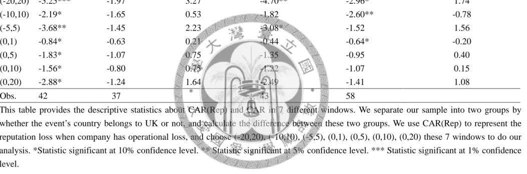
We also separate our samples by country. One is the firms belong to UK another is the firms not belong to UK. From Table 5 we can see the UK events’ CAR(Rep) is more significant negative than the non-UK events’. Especially in the window (-20, 20), the UK events have return -5.25% in CAR(Rep) and -4.70% in CAR. The CAR(Rep)’s

14

difference between UK and non-UK is all positive. From Table 5, UK companies suffer more reputation loss when they have operational loss. These UK companies in our sample adopt the AMA (Advanced Measurement Approaches) to calculate their capital requirement. The AMA approach is stricter than other ways to calculate the capital requirement. So the investors in the market have more sensitivity toward these UK companies when they have operational loss. Compare with other European financial companies, UK financial companies have stricter regulations. That’s why the UK companies suffer more reputation loss when they have operational loss.

4.2.1. Short-term regression result

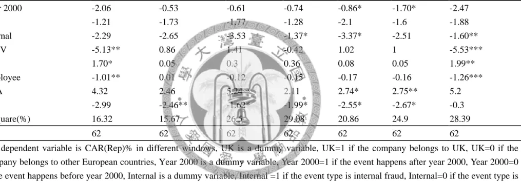
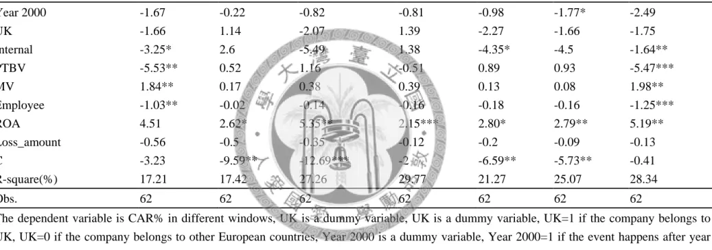
The short-term regression results are presented in Table 6 and Table 7. In Table 6, the dependent variable is CAR(Rep)% in different window. In Table 7, the dependent variable is CAR% in different window. In the CAR(Rep)’s regression result, we focus in the window (0,20). We can see the coefficient of the PTBV is -5.53, which is significant different from zero at the 1% level. It indicates that larger PTBV companies suffer more from the reputation consequences of an operational loss event. Growth firms are more fragile and sensitive to operational loss news. The coefficient of the independent variable Employee is -1.26, which is significant different from zero at the 1% level. The coefficient of the independent variable Internal is -1.60, which is significant different

15

from zero at 5% level. The result is consistent with Perry (2005). They find that market values fall over twice the loss percentage when the loss is due to internal fraud. In our regression result, the negative coefficient of Internal means if the event type is internal fraud, the reputation loss is larger than other event types. The coefficient of the independent variable MV is positive, it means the larger financial firms have less reputation loss when they have operational loss. This result consists with Murphy, Shrieves and Tibbs (2004). They find that firm size is negatively related to the percentage loss in firm market value. They explain that larger company with better brand name may more easily counter the reputational damage.

4.3. Event study result in the long-term

Table 8 shows the long-term performance. In our 101 samples, there are some samples happen after year 2008, so we can’t get the stock price to calculate the two-year BHAR and three-year BHAR. We have 98 samples in two-year BHAR and 87 samples in three-year BHAR. We separate our sample into two ways like the short-term performance: by announcement date and by the firm belongs to UK or not. The three-year BHAR in all-sample is -0.39% which is significant different from zero at the 5% level.

In Table 9, we separate our samples into two groups: the announcement date before

16

year 2000 and after year 2000. We can see clearly the events after year 2000 have worse BHAR than events before year 2000. The three-year BHAR is -1.21% and two-year BHAR is -0.82 which are both significant different from zero at the 1% level when the events happen after year 2000.

In Table 10, we separate our samples into two groups: the firms belong to UK or belong to other European countries. From this table, there is no obvious difference between these two groups. Only three-year BHAR in UK group is -0.82% which is significant different from zero at the 10% level.

4.3.1. Long-term regression result

The long-term performance regression we list in Table 11. We can see the independent variable Year 2000 is significant negative in the long-term, especially when the dependent variable is BHAR(two-year) and BHAR( three-year). It means if a company has operational loss event, the company get more abnormal loss when the event happens after year 2000. The independent variable PTBV and Employee are important in short-term but in the long-term performance seems not so critical from our result. The coefficient of independent variable Internal is negative. It means if the operational loss event type is internal fraud, the operational loss firm’s long-term stock return have worse performance compare with other event types.

17

5. Conclusion

We intend to know how much the operational loss event affects the firm’s reputation in this paper. Reputation is an abstract concept, and we calculate the difference between market value loss and announced loss amount to represent the reputation loss. We focus on European financial companies and do event studies to examine the operational loss firms’ stock price.

We separate our samples by whether the events’ date happen before year 2000 or not, and we find that operational loss companies suffer more reputation loss when the evens date happen after year 2000. Due to our UK-company samples are exceed 40% in our all samples, we try to find the difference between UK-company samples and other European-company samples. So we separate our samples by whether the events’ country belongs to UK or not. We find the UK companies get more reputation loss than other European country companies.

In our short-term regression result, we find that independent variables PTBV plays an important role when we consider the reputation loss in short-term. This independent variable have negative effect on CAR(Rep) and significant. It means higher PTBV firms which are growth firms have more reputation loss when they have operational loss. The independent variables MV has positive relationship with CAR(Rep), it means larger company have less reputation loss when they have operational loss. We explain larger

18

company with better brand name may more easily counter the reputational damage.

From our long-term performance result, we find the events happen after year 2000 have worse performance than the events happen before year 2000. We explain that with the progress of internal control system, the investor in the market have stricter attitude toward operational loss events. We also find the company with operational loss event type is internal fraud have worse performance in the long-term. We think these financial companies should devote a large share of its risk management budget to controlling internal fraud.

19

References

Allen, L., Bali, T.G., 2007. Cyclicality in catastrophic and operational risk measurement.

Journal of Banking and Finance 31, 1191-1235.

Basel Committee, 2003. Sound practices for the management and supervision of operational risk. Bank for International Settlements.

Barber, B.M., Lyon, J.D., 1997. Detecting long-run abnormal stock return: The empirical power and specification of test statistics. Journal of Financial and Economics 43, 341-372.

Chernobai, A., Jorion, P., Yu, F., 2008. The determinants of operational losses. Working paper, Syracuse University.

Cruz, M.G., 2002. Modeling, measuring and hedging operational risk. John Wiley &

Sons, Ltd., New York.

Cummins, J.D., Lewis, C.M., Wei, R., 2006. The market value impact of operational risk events for US banks and insurers. Journal of Banking and Finance 30,605-2634.

de Fontnouvelle, P., DeJesus-Rueff, V., Jordan J., Rosengren E., 2003. Using loss data to quantify operational risk. Working paper, Federal Reserve Bank of Boston .

de Fontnouvelle, P., Jordan J., Rosengren E., 2004. Implication of alternative operational risk modeling techniques. Working paper, Federal Reserve Bank of Boston.

20

de Fontnouvelle, P., DeJesus-Rueff, V., Jordan J., Rosengren E., 2005. Capital and risk:

New evidence on implications of large operational losses. Working paper, Federal Reserve Bank of Boston.

Gillet, R., Hubner G., Plunus, S., 2010. Operational risk and reputation in the financial industry. Journal of Banking and Finance 34, 224-235.

Goddard, J., Molyneux, P., Wilson, J.O.S., Tavakoli, M., 2007. European banking: An overview. Journal of Banking and Finance 20, 745-771.

Hirschey, M., Palmrose, Z.V., Scholz, S., 2005. Long-term market underreaction to accounting restatements. Working paper, University of Kansas.

MacKinlay, A.C., “Event studies in economics and finance,” Journal of Economic Literature, 1997, 35, 13-39.

Mercer Oliver Wyman, 2003. The new rules of game: Implications of the New Basel Capital Accord for the European banking industries, June.

Mitchell, M.L., Erik Stafford, E., 2000. Managerial decisions and long-term stock price performance. Working paper, University of Harvard.

Molyneux, P., Altunbas, Y., Gardener, E.P.M., 1996. Efficiency in European banking.

Journal of Banking and Finance 18, 445-459.

Moscadelli, M., 2004. The modeling of operational risk: Experience with the analysis of the data collected by the basel committee. Technical Report 517, Banca d’Italia.

21

Murphy, D., Shrieves, R.E., Tibbs, S.L., 2004. Determinants of the stock price reaction to allegations of misconduct: Earnings, risk and firm size effect. Working paper, University of Tennessee.

Perry, J., de Fontnouvelle, P., 2005. Measuring reputation risk: The market reaction to operational loss announcement. Working paper, Federal Reserve Bank of Boston.

Uhde, A., Heimeshoff, U., 2009. Consolidation in banking and financial stability in Europe: Empirical evidence. Journal of Banking and Finance 33, 1299-1311.

Williams, J., 2004. Determining management behavior in European banking. Journal of Banking and Finance 28, 2427-2460.

22

Table 1: Events’ loss amount and the number of observations

NO. of obs. NO. of firms Index Loss amount (in Million $)

Mean Min Max

United Kingdom 43 9 FTSE 100 $516.56 $3.91 $17,518.30

France 7 3 CAC 40 $1,175.52 $6.84 $7,162.34

Germany 19 2 DAX $237.97 $3.60 $841.81

Italy 7 5 MIB $229.66 $7.13 $1,188.20

Netherland 7 3 AEX $185.80 $5.19 $456.94

Spain 4 1 IBEX35 $285.91 $43.74 $831.15

Switzerland 14 2 SMI $227.86 $7.38 $922.00

Total 101 25

This table provides the events’ loss amount and the number of observations from year 1990 to year 2010 in our 7 targeted European countries and their corresponding index. The huge operational loss events concentrate in some financial companies. We double check and make sure these events are independent. The highest loss amount is $17518 million and the event company is Lloyds Banking Group. Operational loss amount is at least $3 million because smaller loss is less likely to have influence on the stock price.

23

Table 2: Operational risk loss event types

Event type Obs.

External fraud 20

Internal fraud 20

Clients Products and Business Practices 38

Business Disruption and System Failures 1

Damage to Physical Assets 1

Employment Practices and Workplace Safety 3

Execution Delivery and Process Management 8

Others (Non BIS) 10

Total 101

This table provides the operational risk loss event types which grouped by Basel Committee. External fraud: Losses due to acts of a type intended to defraud, misappropriate property or circumvent the law, by a third party. Internal fraud: Losses due to acts of a type intended to defraud, misappropriate property or circumvent regulations, the law or company policy, excluding diversity and discrimination events, which involve at least one internal party. Clients, Products & Business Practices: Losses arising from an unintentional or negligent failure to meet a professional obligation to specific clients (including fiduciary and suitability requirements), or from the nature or design of a product. Business disruption and system failures: Losses arising from disruption of business or system failures. Damage to Physical Assets: Losses arising from loss or damage to physical assets from natural disaster or other events.

Employment Practices and Workplace Safety: Losses arising from acts inconsistent with employment, health or safety laws or agreements, from payment of personal injury claims, or from diversity / discrimination events. Execution, and Delivery & Process Management: Losses arising from disruption of business or system failures.

24

Table 3: The test statistic for CAR and CAR(Rep)

CAR(Rep) % CAR %

(-20,20) -3.71** -3.70***

(-10,10) -1.94** -2.27***

(-5,5) -2.64** -2.18**

(0,1) -0.75** -0.55

(0,5) -1.47* -1.12*

(0,10) -1.2 -1.13*

(0,20) -2.12* -1.87*

Obs. 79 101

This table provides the descriptive statistics about CAR(Rep) and CAR in 7 different windows. We have 101 samples that have CAR and 79 samples that have CAR(Rep) due to some missing data. We use CAR(Rep) to represent the reputation loss when company has operational loss, and choose (-20,20), (-10,10), (-5,5), (0,1), (0,5), (0,10), (0,20) these 7 windows to do our analysis. *Statistic significant at 10% confidence level.

** Statistic significant at 5% confidence level. *** Statistic significant at 1%

confidence level.

25

Table 4: The test statistic for CAR and CAR(Rep) in sub-sample grouped by year

CAR(Rep)% CAR%

Before year 2000 After year 2000 Difference Before year 2000 After year 2000 Difference

(-20,20) -2.65 -4.65** 1.99 -2.72 -4.27** 1.54

(-10,10) -1.55 -2.28* 0.74 -1.58 -2.66** 1.08

(-5,5) -1.51 -3.63** 2.12** -1.53 -2.56** 1.03*

(0,1) -0.13 -1.29** 1.16 -0.13 -0.80 0.67

(0,5) -0.87 -2.00* 1.13* -0.88 -1.25 0.37

(0,10) 0.11 -2.36*** 2.47** 0.09 -1.84*** 1.93**

(0,20) -1.28 -2.85** 1.57 -1.32 -2.18** 0.87

Obs. 37 42 37 64

This table provides the descriptive statistics about CAR(Rep) and CAR in 7 different windows. We separate our sample into two groups by event’s year, and calculate the difference between these two groups. We use CAR(Rep) to represent the reputation loss when company has operational loss, and choose (-20,20), (-10,10), (-5,5), (0,1), (0,5), (0,10), (0,20) these 7 windows to do our analysis. *Statistic significant at 10%

confidence level. ** Statistic significant at 5% confidence level. *** Statistic significant at 1% confidence level.

26

Table 5: The test statistic for CAR and CAR(Rep) in sub-sample grouped by country

CAR(Rep) % CAR %

UK Others Difference UK Others Difference

(-20,20) -5.25*** -1.97 3.27 -4.70** -2.96* 1.74

(-10,10) -2.19* -1.65 0.53 -1.82 -2.60** -0.78

(-5,5) -3.68** -1.45 2.23 -3.08* -1.52 1.56

(0,1) -0.84* -0.63 0.21 -0.44 -0.64* -0.20

(0,5) -1.83* -1.07 0.75 -1.35 -0.95 0.40

(0,10) -1.56* -0.80 0.75 -1.22 -1.07 0.15

(0,20) -2.88* -1.24 1.64 -2.49 -1.41 1.08

Obs. 42 37 43 58

This table provides the descriptive statistics about CAR(Rep) and CAR in 7 different windows. We separate our sample into two groups by whether the event’s country belongs to UK or not, and calculate the difference between these two groups. We use CAR(Rep) to represent the reputation loss when company has operational loss, and choose (-20,20), (-10,10), (-5,5), (0,1), (0,5), (0,10), (0,20) these 7 windows to do our analysis. *Statistic significant at 10% confidence level. ** Statistic significant at 5% confidence level. *** Statistic significant at 1% confidence level.

27

Table 6: Regression result: Dependent variable is CAR(Rep)

CAR(Rep) %

Dependent variable (-20,20) (-10,10) (-5,5) (0,1) (0,5) (0,10) (0,20)

Year 2000 -2.06 -0.53 -0.61 -0.74 -0.86* -1.70* -2.47

UK -1.21 -1.73 -1.77 -1.28 -2.1 -1.6 -1.88

Internal -2.29 -2.65 -3.53 -1.37* -3.37* -2.51 -1.60**

PTBV -5.13** 0.86 1.41 -0.42 1.02 1 -5.53***

MV 1.70* 0.05 0.3 0.36 0.08 0.05 1.99**

Employee -1.01** 0.01 -0.12 -0.15 -0.17 -0.16 -1.26***

ROA 4.32 2.46 5.24** 2.11 2.74* 2.75** 5.2

C -2.99 -2.46** -1.62* -1.99* -2.55* -2.67* -0.3

R-square(%) 16.32 15.67 26.5 29.08 20.86 24.9 28.39

Obs. 62 62 62 62 62 62 62

The dependent variable is CAR(Rep)% in different windows, UK is a dummy variable, UK=1 if the company belongs to UK, UK=0 if the company belongs to other European countries, Year 2000 is a dummy variable, Year 2000=1 if the event happens after year 2000, Year 2000=0 if the event happens before year 2000, Internal is a dummy variable, Internal =1 if the event type is internal fraud, Internal=0 if the event type is not internal fraud, PTBV is the price-to-book ratio of company on the announcement date, MV is the market value of company on the announcement date, Employee is the number of employees of company on the announcement date, ROA is return on asset of the company on the announcement date, C is constant. *Statistic significant at 10% confidence level. ** Statistic significant at 5% confidence level.*** Statistic significant at 1% confidence level.

28

Table 7: Regression result: Dependent variable is CAR

CAR %

Dependent variable (-20,20) (-10,10) (-5,5) (0,1) (0,5) (0,10) (0,20)

Year 2000 -1.67 -0.22 -0.82 -0.81 -0.98 -1.77* -2.49

UK -1.66 1.14 -2.07 1.39 -2.27 -1.66 -1.75

Internal -3.25* 2.6 -5.49 1.38 -4.35* -4.5 -1.64**

PTBV -5.53** 0.52 1.16 -0.51 0.89 0.93 -5.47***

MV 1.84** 0.17 0.38 0.39 0.13 0.08 1.98**

Employee -1.03** -0.02 -0.14 -0.16 -0.18 -0.16 -1.25***

ROA 4.51 2.62* 5.35** 2.15*** 2.80* 2.79** 5.19**

Loss_amount -0.56 -0.5 -0.35 -0.12 -0.2 -0.09 -0.13

C -3.23 -9.59** -12.69*** -2 -6.59** -5.73** -0.41

R-square(%) 17.21 17.42 27.26 29.77 21.27 25.07 28.34

Obs. 62 62 62 62 62 62 62

The dependent variable is CAR% in different windows, UK is a dummy variable, UK is a dummy variable, UK=1 if the company belongs to UK, UK=0 if the company belongs to other European countries, Year 2000 is a dummy variable, Year 2000=1 if the event happens after year 2000, Year 2000=0 if the event happens before year 2000, Internal is a dummy variable, Internal =1 if the event type is internal fraud, Internal=0 if the event type is not internal fraud, PTBV is the price-to-book ratio of company on the announcement date, MV is the market value of company on the announcement date, Employee is the number of employees of company on the announcement date, ROA is return on asset of the company on the announcement date, Loss_amount is the operational loss amount the company announced, C is constant.*Statistic significant at 10% confidence level. ** Statistic significant at 5% confidence level. *** Statistic significant at 1% confidence level.

29

Table 8: The test statistic for BHAR on three different periods

All-sample Obs.

BHAR( 1Year) -0.20% 101

BHAR( 2Year) -0.25% 98

BHAR( 3Year) -0.39%** 87

This table provides the descriptive statistics about one-year, two-year, and three-year monthly buy-and-hold abnormal return (BHAR). We collect operational loss companies’

monthly return in one-year, two-year, and three-year after the announcement date and compare these stocks’ return with the market index to get the buy-and-hold abnormal return (BHAR). Some events happen after year 2008, so we can’t get enough stock price information to calculate these events’ two-year and three-year BHAR. We have 101 samples in one-year BHAR, 98 samples in two-year BHAR and 87 samples in three-year BHAR. *Statistic significant at 10% confidence level. ** Statistic significant at 5% confidence level. *** Statistic significant at 1% confidence level.

30

Table 9: The test statistic for BHAR in sub-sample grouped by year

Before 2000 Obs. After2000 Obs. Difference

BHAR( 1Year) 0.38% 48 -0.71%* 53 1.09%**

BHAR( 2Year) 0.28% 48 -0.82%*** 30 1.10%**

BHAR( 3Year) 0.21% 48 -1.21%*** 39 1.42%**

This table provides the descriptive statistics about one-year, two-year, and three-year monthly buy-and-hold abnormal return (BHAR) in sub-sample grouped by year. We collect operational loss companies’ monthly return in one-year, two-year, and three-year after the announcement date and compare these stocks’ return with the market index to get the buy-and-hold abnormal return (BHAR). Some events happen after year 2008, so we can’t get enough stock price information to calculate these events’ two-year and three-year BHAR. *Statistic significant at 10% confidence level. ** Statistic significant at 5% confidence level. *** Statistic significant at 1% confidence level.

31

Table 10: The test statistic for BHAR in sub-sample grouped by country

UK Obs. Others Obs. Difference

BHAR( 1Year) -0.44% 40 -0.04% 61 0.40%

BHAR( 2Year) -0.45% 39 -0.12% 59 0.33%

BHAR( 3Year) -0.82%* 34 -0.12% 53 0.70%

This table provides the descriptive statistics about one-year, two-year, and three-year monthly buy-and-hold abnormal return (BHAR) in sub-sample grouped by the company belongs to UK or not. We collect operational loss companies’ monthly return in one-year, two-year, and three-year after the announcement date and compare these stocks’ return with the market index to get the buy-and-hold abnormal return (BHAR).

Some events happen after year 2008, so we can’t get enough stock price information to calculate these events’ two-year and three-year BHAR. *Statistic significant at 10%

confidence level. ** Statistic significant at 5% confidence level. *** Statistic significant at 1% confidence level.

32

Table 11: Regression result: Dependent variable is BHAR%

BHAR%

Dependent variable One-year Two-year Three-year

Year 2000 -1.64* -1.52*** -1.92***

UK -1.52 -0.38 -0.79

Internal -1.04 -0.68 -0.42

PTBV -0.54 -0.32 0.23

MV 0.22** 0.09 -0.23

Employee -0.06 -0.01 0.08

ROA 0.09 0.13 -0.64

Loss_amount -0.42 -0.31 -0.02

C -0.03 1.31** -0.64

R-square(%) 27.54 45.06 49.24

Obs. 59 58 52

The dependent variable is BHAR% in different windows, UK is a dummy variable, UK=1 if the company belongs to UK, UK=0 if the company belongs to other European countries, Year 2000 is a dummy variable, Year 2000=1 if the event happens after year 2000, Year 2000=0 if the event happens before year 2000, Internal is a dummy variable, Internal =1 if the event type is internal fraud, Internal=0 if the event type is not internal fraud, PTBV is the price-to-book ratio of company on the announcement date, MV is the market value of company on the announcement date, Employee is the number of employees of company on the announcement date, ROA is return on asset of the company on the announcement date, Loss_amount is the operational loss amount the company announced, C is constant.*Statistic significant at 10% confidence level. **

Statistic significant at 5% confidence level. *** Statistic significant at 1% confidence level.

33

Figure 1: CAR and CAR(Rep) : All-sample:

This figure shows Cumulated abnormal returns from 20 trading days before the announcement date to 20 trading day after the announcement date in all-sample. The dashed line illustrates the reputation effect.

-4.5%

-4.0%

-3.5%

-3.0%

-2.5%

-2.0%

-1.5%

-1.0%

-0.5%

0.0%

-20 -19 -18 -17 -16 -15 -14 -13 -12 -11 -10 -9 -8 -7 -6 -5 -4 -3 -2 -1 0 1 2 3 4 5 6 7 8 9 10 11 12 13 14 15 16 17 18 19 20

CAR CAR(Rep)

CAR & CAR( Re p )

Days

34

Figure 2: CAR and CAR(Rep) : Events happen before year 2000

This figure shows Cumulated abnormal returns from 20 trading days before the announcement date to 20 trading day after the announcement date in sub-sample: events happen before year 2000. The dashed line illustrates the reputation effect.

-3.0%

-2.5%

-2.0%

-1.5%

-1.0%

-0.5%

0.0%

0.5%

1.0%

-20 -19 -18 -17 -16 -15 -14 -13 -12 -11 -10 -9 -8 -7 -6 -5 -4 -3 -2 -1 0 1 2 3 4 5 6 7 8 9 10 11 12 13 14 15 16 17 18 19 20

CAR CAR(Rep)

CAR & CAR( Re p )

Days

35

Figure 3: CAR and CAR(Rep) : Events happen after year 2000

This figure shows Cumulated abnormal returns from 20 trading days before the announcement date to 20 trading day after the announcement date in sub-sample: events happen after year 2000. The dashed line illustrates the reputation effect.

-6%

-5%

-4%

-3%

-2%

-1%

0%

-20 -19 -18 -17 -16 -15 -14 -13 -12 -11 -10 -9 -8 -7 -6 -5 -4 -3 -2 -1 0 1 2 3 4 5 6 7 8 9 10 11 12 13 14 15 16 17 18 19 20

CAR CAR(Rep)

CAR & CAR( Re p )

Days

36

Figure 4: CAR and CAR(Rep) : Event firms belong to UK.

This figure shows Cumulated abnormal returns from 20 trading days before the announcement date to 20 trading day after the announcement date in sub-sample: the company belongs to UK. The dashed line illustrates the reputation effect.

-6%

-5%

-4%

-3%

-2%

-1%

0%

-20 -19 -18 -17 -16 -15 -14 -13 -12 -11 -10 -9 -8 -7 -6 -5 -4 -3 -2 -1 0 1 2 3 4 5 6 7 8 9 10 11 12 13 14 15 16 17 18 19 20

CAR CAR(Rep)

CAR & CAR( Re p )

Days

37

Figure 5: CAR and CAR(Rep) : Event firms belong to other European countries

This figure shows Cumulated abnormal returns from 20 trading days before the announcement date to 20 trading day after the announcement date in sub-sample: the company belongs to other European countries. The dashed line illustrates the reputation effect.

-6%

-5%

-4%

-3%

-2%

-1%

0%

-20 -19 -18 -17 -16 -15 -14 -13 -12 -11 -10 -9 -8 -7 -6 -5 -4 -3 -2 -1 0 1 2 3 4 5 6 7 8 9 10 11 12 13 14 15 16 17 18 19 20

CAR CAR(Rep)

CAR & CAR( Re p )

Days