A Distributed Approximation for Multi-Hop Clustering Problem in Wireless Sensor Networks
Xudong Zhu∗, Jun Li∗, Xiaofeng Gao∗§, Fan Wu∗, Guihai Chen∗, Athanasios V. Vasilakos†
∗Shanghai Key Laboratory of Scalable Computing and Systems, Department of Computer Science and Engineering, Shanghai Jiao Tong University, Shanghai, 200240, China
†Dept of Computer Science, Electrical and Space Engineering, Lulea University of Technology, Lulea, 97187, Sweden
[email protected], [email protected], {gao-xf, fwu, gchen}@cs.sjtu.edu.cn, [email protected]
Abstract—In wireless sensor networks (WSNs), there is no pre- defined infrastructure. Nodes need to frequently flood messages to discover routes, which badly decreases the network performance.
To overcome such drawbacks, WSNs are often grouped into several disjointed clusters, each with a representative cluster head (CH) in charge of the routing process. In order to further improve the efficiency of WSNs, it is crucial to find a cluster partition with minimum number of clusters and the distance between each node to its corresponding CH can be bounded by a constant number of hops. Finding such a partition is defined as minimum d-hop cluster head set (d-MCHS) problem, which is proved to be NP-hard. In this paper, we propose a distributed approximation algorithm, named d2-Cluster, to address d-MCHS problem and prove that the approximation ratio of d2-Cluster under unit disk graph (UDG) is a constant factor λ which is related to d. To the best of our knowledge, it is the first constant approximation ratio for d-MDS problem in UDG.
I. INTRODUCTION
Wireless sensor networks (WSNs) is a kind of autonomous communication systems with lots of small-sized, inexpensive and battery-powered sensors. Since such sensors are cheap and can be deployed in various environments, WSNs have been widely used in many applications, such as monitoring, disaster management, battlefield surveillance, etc. [1]–[3].
Usually the most important task for a sensor is to gather its surrounding information and send its data to the nearest sink. However, in WSNs, there is no fixed or predefined in- frastructure. If a sensor wants to communicate with a specified peer, it needs to discover the route between them by flooding messages. This mechanism causes a lot of serious problems, such as traffic collision, energy consumption, etc.
In order to overcome these shortcomings, an efficient ap- proach named clustering is widely pursued by the research
§X.Gao is the corresponding author.
This work has been supported in part by the National Natural Sci- ence Foundation of China (Grant number 61202024, 61472252, 61133006, 61422208), China 973 project (2012CB316200), the Natural Science Founda- tion of Shanghai (Grant No.12ZR1445000), Shanghai Educational Develop- ment Foundation (Chenguang Grant No.12CG09), Shanghai Pujiang Program 13PJ1403900, and in part by Jiangsu Future Network Research Project No.
BY2013095-1-10 and CCF-Tencent Open Fund.
community. We can partition a given WSN into several dis- jointed clusters, each of which is a small-scale autonomous communication system. Specially, each cluster has a leader, called cluster head (CH). A CH is the interface for ordinary sensors in the corresponding cluster to contact the outsides.
With clustering technique, an ordinary sensor only needs to focus on gathering information and sending the data to its CH, and its CH will forward the data to the sink outside.
Obviously, this mechanism can save a lot of energy and reduce the number of collisions by avoiding many redundant message forwardings.
In the literature, many clustering algorithms were proposed for WSNs. In [4], Younis et al. devised a clustering algorithm to achieve equal-sized clusters to balance the work load of each cluster. In [5], Demirbas et al. presented a clustering algorithm, named FLOC, to partition a WSN into non-overlapping and approximately equal-sized clusters. Since each cluster is equal- sized, CHs take charge for a same amount of sensors. However, there still exists a serious problem. Some ordinary sensors in a cluster may be too far away from the CH, which will take a long route when transmitting data to the CH. As a consequence, it downgrades the performance of the cluster strategy. On contrast, Wang et al. studied the problem of minimizing the average hop distance from any node to its cluster head in 2D sensor networks in [6]. However, they did not consider to control the sizes of clusters when partitioning a WSN, which will causes load imbalance among cluster heads.
To solve the conflicts above, an effective approach is to set a parameter d, and for each node in a cluster, the hop distance between it to its CH is upper bounded by d. Since every sensor in a cluster is within d hops from its CH, the CH can manage this cluster efficiently. Besides, since sensors are usually deployed randomly in lots of applications, this approach can also effectively obtain approximately equal-sized cluster. Moreover, the average size of clusters can be controlled by setting different values of d.
In this paper, we focus on partitioning a WSN into the minimum number of d-hop clusters. Here, a d-hop cluster means each sensor in it is either a CH or within d hops
from the CH. Obviously, finding such a partition is to find a minimum d-hop cluster head set (d-MCHS), because a cluster is determined once the CH is determined. Moreover, for simplicity, we often use a graph to model a WSN. It is not difficult to observe that finding a d-MCHS in a WSN is to find a minimum d-hop dominating set (d-MDS) in the corresponding graph. In this paper, we propose a distributed d-hop clustering algorithm (d2-Cluster), to address d-MCHS problem. d2-Cluster is a degree-based algorithm. With local information of neighbors within 2d hops, each sensor decides whether it can be selected as a CH. Our contributions in this paper are summarized as follows.
• Since WSNs are self-organized distributed system, we de- vise an efficient distributed algorithm, named d2-Cluster, to address d-MCHS problem. Moreover, d2-Cluster is valid under any network model.
• As d2-Cluster is an approximation for d-MCHS problem, we prove that the approximation ratio of d2-Cluster under UDG model is λ, which is a constant factor given in Section IV.
• We discuss the time complexity and message complexity of d2-Cluster. From simulation results, we show that d2- Cluster is almost as fast as the previous fastest distributed algorithm.
Our paper is organized as follows. In Section II provides some preliminaries. We describe our algorithm d2-Cluster for d-MCHS problem in Section III. Section IV provides the analysis of our algorithm and illustrates the simulation. Finally, Section V concludes this paper.
II. PRELIMINARIES
To simplify our problem, we assume: (1) The networks we discuss in this paper are homogeneous networks; (2) We ignore collisions of signals during the procedure of message transmitting. With these assumptions, we have the following definitions for a given graph G = (V, E).
Definition 1 (d-IS). A subset S ⊆ V is a d-hop Independent Set (d-IS) of G if ∀u, v ∈ I, there does not exist a path within d hops between u and v.
Definition 2 (d-MIS). A d-IS is a d-hop Maximal Independent Set (d-MIS) if ∀u ∈ V \I, I ∪ {u} is no longer a d-IS.
Definition 3 (d-DS). A subset D ⊆ V is a d-hop Dominating Set (d-DS) of G if ∀u ∈ V , either u ∈ D or ∃v ∈ D such that there exists a path within d hops between u and v.
According to Definition 2 and Definition 3, it is easy to get the following Lemma.
Lemma 1. For any given graph G, a d-MIS is also a d-DS.
Next, we formalize our problem in this paper as follows.
Definition 4 (d-MCHS Problem). Given a WSN that is mod- eled as a graph G = (V, E), finding a d-hop cluster head set (d-CHS) from the WSN, namely finding a d-DS from G, with minimum size is called d-MCHS problem.
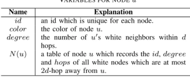
TABLE I VARIABLES FOR NODEu
Name Explanation
id an id which is unique for each node.
color the color of node u.
degree the number of u0s white neighbors within d hops.
N (u) a table of node u which records the id, degree and hops of all white nodes which are at most 2d-hop away from u.
The problem of finding a minimum dominating set (MDS) is NP-hard even in UDG [7]. Since MDS problem is a special case of d-MCHS problem, d-MCHS problem is also NP-hard.
III. d2-CLUSTER FORd-MCHSPROBLEM
Since d-MCHS problem is NP-hard, we can not find an optimal solution in polynomial time unless NP = P. With Lemma 1, we can construct a d-DS by selecting a d-MIS from G as an approximation for d-MCHS. To make this approximation more efficient, the size of the d-MIS should be as small as possible. Based on this idea, we designed our distributed algorithm, named d2-Cluster, for d-MCHS problem.
According to the definition of d-MIS, the hop distance between any two nodes in a d-MIS is more than d. Moreover, we observe that, for any d-MIS node u, if the hop distance between u to its nearest d-MIS node is larger, it shall be better to reduce the size of d-MIS. Hence, the restriction in [8] that every d-MIS node is d + 1 hops away from its nearest d-MIS node is an obstacle in terms of reducing the size of d-MIS.
Removing such restriction does help reduce the size of d-MIS.
Besides, it is not difficult to observe that any d-MIS node can be separated from its nearest d-MIS node by at most 2d+1 hops. As a consequence, it is sufficient for a node to compare itself with nodes that are at most 2d hops away from itself, to decide whether it should be selected as a CH. Based on this, we propose a degree-based distributed algorithm to construct a smaller d-MIS for a given graph.
During the process of our algorithm, each node maintains several variables which are listed in Table I. For node u, u.color reflects its current status. There are three different kinds of color, which are white, black and grey. Initially, every node is colored white. Once a node is chosen as a CH, it changes its color to black. If a node’s color is grey, it means there exist at least one CH within d hops from this node. u.degree means the number of u’s white neighbors within d hops. For N (u), each element in it is a triple (id, degree, hops) and corresponds to a white node within 2d hops from u, say v. Then, for this triple, id is the id number of node v, degree is the value of v.degree and hops is the hop distance between u and v.
d2-Cluster consists of two phases. The first phase is to initialize the variables for each node. The second phase is to color nodes black or grey according to their local information stored in N (·).
Algorithm 1: Initialization
1 u.color = white, u.degree = 0, N (u) = ∅;
2 Broadcast a HELLO(u.id, 1) message;
3 After N (u) collects all its neighbors within 2d hops,
4 foreach e ∈ N (u) do
5 if e.hops ≤ d then
6 u.degree = u.degree + 1;
7 end
8 end
9 Broadcast an NEW DEG(u.id, u.degree, 1) message;
When receiving HELLO(i, h):
10 if u.id 6= i then
11 if ∃e ∈ N (u) s.t. e.id = i then
12 if e.hops > h then
13 e.hops = h;
14 if h < 2d then
15 Broadcast HELLO(i, h + 1);
16 end
17 end
18 else
19 Push (i, 1, h) into N (u);
20 if h < 2d then
21 Broadcast HELLO(i, h + 1);
22 end
23 end
24 end
When receiving NEW_DEG(i, degree, h):
25 if degree 6= e.degree, where e ∈ N (u) and e.id = i then
26 e.degree = degree;
27 if h < 2d then
28 Broadcast NEW DEG(i, degree, h + 1);
29 end
30 end
A. Initialization
In this phase, each node initializes its variables by broad- casting messages HELLO and NEW DEG. The corresponding specifications of these messages are as follows.
• HELLO: Each node broadcasts this kind of message to inform its neighbors its presence. This kind of message contains two parameters, id and hops. id means the id number of the node from which the current HELLO message originates from. We call that node as the original node. hops means the hop distance between the receiving node and the original node.
• NEW DEG: When a node’s degree changes, it broad- casts this kind of message to inform its 2d-hop neighbors to update their local informations. This kind of message contains three parameters: id, degree and hops. id is the id number of the original node of this message. hops is the hop distance between the receiving node and the original node. degree is the new value of the original node’s degree.
Initially, each node broadcasts a HELLO(id, 1) message to show its presence and each of its 1-hop neighbors forwards this massage by broadcasting message HELLO(id, 2). Generally, when a node receives a HELLO(i, h) message, it will forward it by broadcasting a HELLO(i, h + 1) if h < 2d. In this way, after node u broadcasts HELLO(u.id, 1), every node which is at most 2d hops away from u will know u0s presence.
When each node ascertains that its variable N (·) has recorded all its neighbors within 2d hops, it updates its degree by checking the information in N (·). However, all its neighbors within 2d hops only record that its degree is 1 (Line 19). Thus, it broadcasts an NEW DEG message to inform all its neighbors within 2d hops this change. The detailed description is shown in Alg. 1.
B. d-MIS Construction
In this phase, d2-Cluster selectes a d-MIS by coloring some white nodes black, and the detailed description is shown in Alg. 2, As Alg. 2 shows, this algorithm is executed round by round. At the beginning of each round, for any node u, if u.color is white, it will check the degrees of its white neighbors within 2d hops, which are stored in N (u). When u has the lowest rank compared with any node in N (u), it will be selected as a CH and colored black. Here, for any two nodes u and v, u has a lower rank iff one of the following conditions meets:
• u.degree > v.degree,
• u.degree = v.degree and u.id < v.id.
Once u is colored black, all its white neighbors within d hops will be colored grey. These black and grey nodes are added into a set S. Then, u spreads S up to 3d hops, because nodes in that region may need to update their local information, such as degree and N (·). After that, u terminates.
Besides, at the beginning of each round, if N (u) is an empty set, u will also terminate. The time interval between two adjacent rounds is previously set to be long enough, so that all those updating works can be done in each round.
In the procedure of Alg. 2, it also involves two kinds of messages, BLACK and NEW DEG. The specification of BLACK message is similar with HELLO message.
Fig. 1 shows an example to illustrate the procedure of d2- Cluster. In this example, d = 2. d2-Cluster selects nodes 4, 11, 17 as a 2-MIS.
IV. ALGORITHMANALYSIS
In this section, we mainly analyze the approximation per- formance and the complexity of d2-Cluster under UDG model.
A. Approximation Ratio Analysis
We first introduce some notations that will be used in this subsection. For any graph G, G is a unit disk graph (UDG) if ∀u, v ∈ V , (u, v) ∈ E iff the Euclidean distance between u and v is at most 1. In a unit disk graph G = (V, E), for any node u ∈ V , let Nr(u) denote the set of nodes which are at most r hops away from u. Let diskr(u) denote the disk with center u and radius r. Let |S| denote the cardinality of set S.
Algorithm 2: Distributed d-MIS Construction (per round)
1 if N (u) = ∅ then
2 if u.color = white then
3 u.color = black;
4 Broadcast BLACK(u.id, {u}, d + 1);
5 end
6 Terminate;
7 end
8 if u.color = white and u has the lowest rank compared with any node inN (u) then
9 u.color = black;
10 S = {u};
11 foreach e0∈ N (u) do
12 if e0.hops ≤ d then
13 Push e0.id into S;
14 end
15 end
16 Broadcast BLACK(u.id, S, 1);
17 Terminate;
18 end
When receiving BLACK(i, S, h):
19 cnt = 0, f lag = 0;
20 foreach e0∈ N (u) do
21 if e0.id ∈ S then
22 if e0.hops ≤ d then
23 cnt = cnt + 1;
24 end
25 Remove e0, f lag = 1;
26 end
27 end
28 if h ≤ d and u.color = white then
29 if u.color = white then
30 u.color = grey;
31 end
32 end
33 else if h ≤ 2d then
34 u.degree = u.degree − cnt;
35 Broadcast NEW DEG(u.id, u.degree, 1);
36 end
37 if h < 3d and f lag = 1 then
38 Broadcast BLACK(i, S, h + 1);
39 end
When receiving NEW_DEG(i, degree, h):
40 if degree 6= e.degree, where e ∈ N (u) and e.id = i then
41 e.degree = degree;
42 if d < 2d then
43 Broadcast NEW DEG(i, degree, h + 1);
44 end
45 end
First, we only discuss one cluster in G = (V, E) and denote it by Cluster(o), where o is the CH of this cluster. Then, every node in Cluster(o) is within d hops away from o. Next,
we analyze how many d-hop independent nodes there are in Cluster(o). Denote that number as α. In order to prove an upper bound for α, we introduce the following Lemma.
Lemma 2. (Zassenhaus-Groemer-Oler inequality) [9]. The number of non-overlapping disks with radius 0.5 whose cen- ters can be packed into a compact convex regionC is bounded by
√2
3A(C) +1
2P (C) + 1,
where A(C) and P (C) are the area and perimeter of C, respectively.
From Lemma 2, we can immediately conclude the following corollary.
Corollary 1. diskr(o) can contain at most 2
√3πr2+ πr + 1 independent nodes.
It is easy to find that all those d-hop independent nodes in Cluster(o) are located in diskd(o). Additionally, the Euclidean distance between any two d-hop independent nodes is greater than 1. According to Corollary 1, we have
α ≤ 2
√
3πd2+ πd + 1. (1)
However, this is a rough estimation for α. Inspired by [11], we can improve it further.
When d = 1, it is easy to figure out that α ≤ 5 because a unit disk can contains at most 5 independent nodes. When d = 2, α ≤ 21 by inequality (1). Next, we only discuss the situations where d ≥ 3. Assume I is the set of d-hop independent nodes in Cluster(o). We partition I into two parts as follows:
A = Ndd/2e(o) ∩ I = {u1, u2, . . . , ut} B = Nd(o)\Ndd/2e(o) ∩ I = {v1, v2, . . . , vs} For the first part, we are to show that t ≤ 5.
Suppose t > 5. Since N1(o) contains at most 5 independent nodes, we could always find two nodes uiand uj so that their last nodes on their shortest paths to o are not independent.
Thus, there exists a path with length of at most 2(dd/2e − 1) + 1 ≤ d between ui and uj. Consequently, ui and uj are not d-hop independent, which yields a contradiction.
For the second part, denote the shortest path from vi to o as Pi, where 1 ≤ i ≤ s. Let Si= Nb(d−1)/2c(vi) ∩ Pi. Consider two nodes vi, vj ∈ B. For any two nodes w ∈ Si, z ∈ Sj, it is clear that they are not adjacent. Otherwise, there exists a path vi w→z vj with length of at most 2b(d − 1)/2c + 1 ≤ d, which yields a contradiction. Since Piis the shortest path from vi to o, any node in Pi is not adjacent to its second succes- sor and predecessor. Thus, Si contains at least d1
2bd − 1 2 ce disjointed nodes. Assume Ai ⊆ Si and any two nodes in Ai are not adjacent. Then, |Ai| ≥ d1
2bd − 1
2 ce. Besides,
(a). Initialization (b). After the first round of Alg. 2 (c). After the second round of Alg. 2
Fig. 1. An example to illustrate d2-Cluster. (a) shows the input graph of a 2-MCHS problem with 18 nodes. At the beginning of the first round in Alg. 2, each node has initialized its local variables. By checking its degree with its white neighbors within 4 hops, nodes 4 and 11 are selected as cluster heads.
Then, nodes 4 and 11 are colored black and their neighbors within 2 hops are colored grey. The state after the first round is shown in (b). At the beginning of the second round, there are only three white nodes. By checking, node 17 is selected as CH and colored black. Its white neighbors (nodes 16, 18) are colored grey. The state of all nodes is shown in (c). Since all nodes are colored black or grey, Alg. 2 teminates.
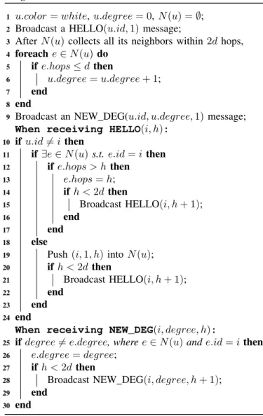
(a). Rounds for d2-Cluster and algorithm in [10] (b). Rounds of d2-Cluster for larger d (c). The output size of d-MIS.
Fig. 2. Comparison between d2-Cluster and Alg. in [10] in terms of time complexity
any two nodes in Ai∪ Aj are also not adjacent. Combining Inequality (1), we have
s ≤ α
d1 2bd − 1
2 ce
≤
√2
3πd2+ πd + 1 d1
2bd − 1 2 ce
.
Based on the analysis above, we can conclude an improved upper bound for α. We denote it by λ and
λ =
5, if d = 1,
21, if d = 2,
5 +
√2
3πd2+ πd + 1
d12bd−12 ce , if d ≥ 3.
Assume that the size of d-MCHS is opt. Then, there are no more than λopt d-hop independent nodes in graph G. Aslo d2- Cluster cannot select more than λopt black nodes. Therefore, we have the following theorem.
Theorem 1. d2-Cluster has an approximation ratio ofλ under UDG model.
B. Complexity Discussion ford2-Cluster
Since d2-Cluster is a synchronous distributed algorithm, we consider two typical kinds of complexity: message complexity and time complexity. It is easy to see that the message complexity of d2-Cluster is O(n2). As for time complexity, we will first give a loose upper bound for general graphs.
Then, we will compare d2-Cluster under UDG model with the previous best algorithm [10] in terms of time complexity.
Typically, for a distributed algorithm, we measure its time complexity by the number of rounds each node runs during its executing process. As for Alg. 1, it can be finished in only one round. Hence, the time complexity of Alg. 1 is O(1). As for Alg. 2, obviously the whole algorithm terminates when all nodes are colored black or grey. In each round, there is at least one white node that will be colored black, and all its white neighbors that are at most d hops away from it will be colored grey. In the worst case, the number of rounds in Alg. 2 is O(n). Therefore, the time complexity of d2-Cluster for general graphs is O(n).
In [10], the authors proposed a distributed algorithm for MIS problem in bounded-independence graphs. As far as we know, their algorithm is the fastest distributed algorithm. With time complexity O(log∗n). To compare d2-Cluster with that fastest algorithm, we make some related simulations in UDG model and the results are shown in Fig. 2. Since [10] only discussed finding an MIS, we compare its results when d = 1.
In our simulations here, all nodes are randomly located on a two-dimensional virtual region. The range of the region is 20 × 20. For each node, its sensing range is 1. The number of nodes are from 50 to 1000. For each data in these figures, we run the corresponding simulations 50 times and take their average value as the final data.
From Fig. 2(a), we can see that Alg. in [10] is faster than d2-Cluster. However, the difference between them is not
(a). The size of d-MIS vs. the size of networks (b). The average size of clusters (c). The overlaps between clusters Fig. 3. Simulation results for evaluating the performance of d2-Cluster
quite large. In other words, the time complexities for both algorithms are of the same order of magnitude. In this sense, d2-Cluster is almost as fast as the algorithm in [10]. From Fig. 2(b), for d2-Cluster, the number of rounds decreases with large d when the number of nodes is not large enough. These results are reasonable, because each dominator can cover more nodes when d increases. When the number of nodes keeps on increasing, the numbers of rounds for d = 2, 4, 6 are almost the same.
The curve even becomes more flat with larger size of networks. According to Fig. 2(c), we can see that d2-Cluster can select a smaller-sized MIS compared with the algorithm in [10]. In this sense, d2-Cluster is more efficient than the algorithm in [10].
C. More Numerical Experiments
We evaluate the performance of d2-Cluster for partitioning wireless sensor networks by simulations. In our simulations, sensor nodes are randomly generated in a 2D virtual space.
The number of sensors varies from 50 to 1000 at intervals of 50. All the experiments are performed 100 times and the average results are taken. First, we studied the size of d- MIS obtained by d2-Cluster. In addition, we also studied the average size of clusters and the overlapping ratio between clusters. The simulation results are as follows.
Fig. 3(a) shows the number of d-MIS obtained by d2- Cluster, where d = 2, 3, 4. From this figure, we can see that the size of d-MIS reduces with increasing d.
From Fig. 3(b), we can see that the average size of clusters tends to be stable when the size of networks increases. More- over, the stable value of the average size is nearly proportional to d2. In this sense, we can effectively control the average size of clusters by changing the value of d.
As for the overlapping ratio, we consider the nodes which are located in at least two clusters. We call those nodes as overlapping nodes. Obviously, these overlapping nodes can be of great use in lots of applications, such as routing between clusters and recovery from cluster head failure. From Fig. 3(c), we can see that the overlapping nodes are about 27%, which is appropriate for those applications.
From these simulation results, we can conclude that d2- Cluster is an effective clustering algorithm for WSNs partition.
V. CONCLUSION
In this paper, we studied the multi-hop clustering problem for a given wireless sensor network, which is defined as d- MCHS problem. We presented a distributed, approximation algorithm, named d2-Cluster, to address d-MCHS problem. d2- Cluster is a degree-based algorithm. Each node uses the local information of its neighbors within 2d hops to decide whether it can be selected as a cluster head (CH). We discussed its time complexity and message complexity. For time complexity, we compared d2-Cluster with the previous fastest algorithm under UDG model and we showed that d2-Cluster is almost as fast as the previous fastest algorithm. Moreover, we also proved the performance ratio of d2-Cluster under UDG model is λ, where λ is a constant parameter related to d. As far as we know, this is the first constant result for d-MDS problem in UDG.
Finally, the simulation results also showed the high efficiency of d2-Cluster.
REFERENCES
[1] S. Basagni, L. Boloni, P. Gjanci, C. Petrioli, C. A. Phillips, and D. Turgut, “Maximizing the value of sensed information in underwater wireless sensor networks via an autonomous underwater vehicle,” in IEEE INFOCOM. IEEE, 2014, pp. 988–996.
[2] I. Benkhelifa, N. Nouali-Taboudjemat, and S. Moussaoui, “Disaster man- agement projects using wireless sensor networks: An overview,” in Ad- vanced Information Networking and Applications Workshops (WAINA).
IEEE, 2014, pp. 605–610.
[3] B. Pannetier, J. Dezert, and G. Sella, “Multiple target tracking with wireless sensor network for ground battlefield surveillance,” in IEEE FUSION. IEEE, 2014, pp. 1–8.
[4] O. Younis and S. Fahmy, “Heed: a hybrid, energy-efficient, distributed clustering approach for ad hoc sensor networks,” IEEE Transactions on Mobile Computing, vol. 3, no. 4, pp. 366–379, 2004.
[5] M. Demirbas, A. Arora, and V. Mittal, “Floc: A fast local clustering service for wireless sensor networks,” in DIWANS/DSN, 2004.
[6] W. Wang, D. Kim, N. Sohaee, C. Ma, and W. Wu, “A PTAS for minimum d-hop underwater sink placement problem in 2d underwater sensor networks,” Discrete Mathematics, Algorithms and Applications, vol. 1, no. 2, pp. 283–289, 2009.
[7] B. N. Clark, C. J. Colbourn, and D. S. Johnson, “Unit disk graphs,”
Annals of Discrete Mathematics, vol. 48, pp. 165–177, 1991.
[8] P.-J. Wan, K. M. Alzoubi, and O. Frieder, “Distributed construction of connected dominating set in wireless ad hoc networks,” in IEEE INFOCOM 2002, vol. 3, 2002.
[9] N. Oler, “An inequality in the geometry of numbers,” Acta Mathematica, vol. 105, no. 1, pp. 19–48, 1961.
[10] J. Schneider and R. Wattenhofer, “An optimal maximal independent set algorithm for bounded-independence graphs,” Distributed Computing, vol. 22, no. 5-6, pp. 349–361, 2010.
[11] Z. Zhang, Q. Liu, and D. Li, “Two algorithms for connected r-hop k- dominating set,” Discrete Mathematics, Algorithms and Applications, vol. 1, no. 04, pp. 485–498, 2009.
![Fig. 2. Comparison between d 2 -Cluster and Alg. in [10] in terms of time complexity](https://thumb-ap.123doks.com/thumbv2/9libinfo/9654759.678116/5.918.97.820.322.490/fig-comparison-d-cluster-alg-terms-time-complexity.webp)
