國立臺灣大學電機資訊學院網路與多媒體研究所 碩士論文
Graduate Institute of Networking and Multimedia College of Electrical Engineering and Computer Science
National Taiwan University Master Thesis
學習基於異質性網路的領域感知網路表示法 Field-aware Network Embedding on Heterogeneous
Networks
陳心萍 Hsin-Ping Chen
指導教授:鄭卜壬博士 Advisor: Pu-Jen Cheng, Ph.D.
中華民國 106 年 6 月
June, 2017
誌謝
感謝在我碩士生涯中幫助我的指導教授——鄭卜壬、實驗室同學、
朋友以及陪伴我的家人。在這段時間裡,從老師身上,不只學習到如 何切入研究問題,設計模型和實驗,並且找到適合自己的研究方向。
實驗室的氣氛良好,他們是可以一起討論研究,和課業,也是一起玩 的好夥伴,真心感謝能在碩士期間能有他們的陪伴。最後感謝一直陪 伴我,給予我幫助的,像我第二顆 CPU 的男朋友,感謝有你。碩士畢 業是我人生的一個重要的里程碑,也是開啟我下一段生活的新起點。
中文摘要
學習網路表示法技術是目前很熱門的研究主題,此技術從複雜的網 路結構學習出低維度的表示法代表節點,此表示法除了保留網路結構 的關係外,讓網路中的節點能做向量的運算,對於後續的機器學習問 題提供較高的基礎,像是多分類問題、預測問題和推薦問題。但是目 前的學習網路表示法技術並不能很好的應用在異質性的網路中,因為 異質性網路包含不同類別的節點與多種類別關係,學習後的表示法來 自於不同的向量空間不能比較。基於這個原因,本篇研究將領域感知 的概念應用在學習表示法技術,希望利用這種概念改善學習網路表示 法技術在異質性網路中無法學習出可以比較的向量問題。本研究也應 用在多個生活中的資料集,實驗證明,本研究不只能保留異質性網的 關係,對於後續的機器學習問題也能有好的成果。
Abstract
Network embedding is used for extracting the feature representations of a network and benefits many machine learning tasks, such as classification, link prediction, etc. This model embeds the interactions among the vertices into the low-dimension representations, which greatly preserve the relations of the vertices. However, to simplify the learning procedure, most previous work treats all the vertices as the same type and thus ignores the interaction type of two vertices in different fields. In the light of this, we propose a field- aware network embedding model which can separately embed the distinct kinds of the interactions into the learned representations. Our experimental results show that integrating such field-aware information indeed improves the performance of the state-of-the-art network embedding algorithm.
Contents
口試委員會審定書 i
誌謝 ii
中文摘要 iii
Abstract iv
1 Introduction 1
2 Related Works 5
2.1 The idea of field-aware . . . 5
2.2 Network Embedding algorithms . . . 6
2.3 Heterogeneous Networks . . . 7
3 Methodology 8 3.1 Problem Definition . . . 8
3.2 Field-aware embedding structure . . . 9
3.3 Model Description . . . 11
3.4 Model Optimization . . . 12
4 Experiments 14 4.1 Dataset . . . 14
4.2 Compared Algorithms . . . 16
4.3 Evaluation Metrics . . . 16
4.4 Parameter Settings . . . 17
4.5 Experiment Results . . . 18
4.5.1 Network Reconstruction . . . 18
4.5.2 Multi-label Classification . . . 20
4.5.3 Link Prediction / Item Recommendations . . . 21
4.5.4 Documents Classification . . . 22
4.5.5 Experiment Results Summary . . . 22
5 Discussion 23 5.1 Parameter Sensitive . . . 23
5.1.1 Performance w.r.t. #Samples . . . 23
5.1.2 Performance w.r.t. Dimension . . . 23
5.1.3 Performance w.r.t. Network Sparsity . . . 24
5.2 Dimension of Fields . . . 25
6 Conclusion 27
Bibliography 28
List of Figures
1.1 The diagram of network embedding. . . 1
1.2 The diagram of heterogeneous network . . . 2
1.3 The goal of field-aware network embedding. . . 4
3.1 The diagram of Multi-Representation Multi-Context . . . 9
3.2 The diagram of Multi-Representation Single-Context . . . 10
4.1 The 2-dimensional representations obtained from each baseline model on Movielens-1m. . . 18
5.1 The performance of two machine learning applications w.r.t. #samples on Movielens-1m datasets. . . 24
5.2 The multi-label classification result w.r.t. Dimension on three datasets. . . 25
5.3 The multi-label classification result w.r.t. Degree of vertices on three datasets. . . 25
5.4 The performance w.r.t User-Movie dimensions on ML-1m. . . 26
List of Tables
4.1 Statistics of the real-world network datasets. . . 15 4.2 Statistics of the language networks. . . 16 4.3 The network reconstruction results in Movielens datasets (1m & 10m) . . 19 4.4 The network reconstruction results in Last.fm . . . 19 4.5 The multi-label classification results in Movielens datasets (1m & 10m). . 20 4.6 The multi-label classification results in Last.fm. . . 20 4.7 The item recommendation results in Movielens datasets (1m & 10m). . . 21 4.8 The item recommendation results in Last.fm. . . 21 4.9 The documents classification results on 20 newsgroup and DBLP datasets. 22
Chapter 1 Introduction
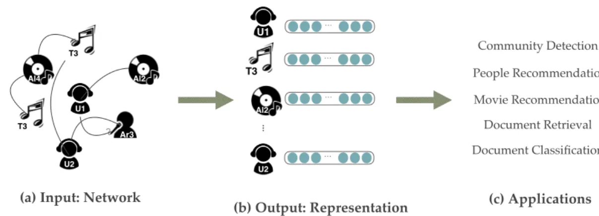
Network embedding is used to learn low dimension feature representation of the ver- tices from a information network. The low dimension vectors are useful in many machine learning applications. For instance, in a social network, the user-user relations can be com- pressed into the learned representations, so it is possible to apply the group detection or people recommendations on the obtained representations. In the movie recommendation task, the embedding model can generate the low-dimension vectors based on the given user-song network, so it is able to recommend a list of movies to a specific user according what he/she likes in before. Figure 1.1 shows the diagram of network embedding usage.
In short, given a relation network, the learned representations are beneficial to variant data prediction tasks.
Al4
U1
U2
Ar3 T3
T3
...
…
…
…
…
U1
Al2 T3
U2
(a) Input: Network
(b) Output: Representation (c) Applications
Al2
Community Detection People Recommendation Movie Recommendation
Document Classification Document Retrieval
Figure 1.1: The diagram of network embedding.
In the literature, a number of network embedding models have been proposed to learn the feature representation. Graph factorization [2, 3] uses the matrix factorization to model the interactions among the objects in a graph network so that the factorized latent vectors represents the learned representations. DeepWalk [15] exploits the random walk to sample the data relations from the network and use the skip-gram model to learn the representa- tions. LINE [20] is the first attempt to preserve both the local and global network structure in the representations. In summary, the core of building a network embedding model is to determine which vertices are considered to be similar and which vertices are considered to be dissimilar. Given a relation network, the proposed model adopts the two criteria 1) the vertices which are connected to each other are similar to each other and 2) the vertices which share the common neighbor vertices are similar to each other.
Al4
U1
U2
Al2
Ar3 T3
T3
(a) User - Music Network (Type: User, Music, Album, Artist)
(b) User - Movie Network (Type: User, Movie, Actor, Director)
M1
M2 Act6 U4
U7 U1
Figure 1.2: The diagram of heterogeneous network
In a real word dataset, the given network usually contains various types of vertices, which can be referred to figure 1.2. To cite examples, in a play-list recommendation problem [6], the dataset may contain the users, the tracks, the albums, the artists, ... etc, which can be referred to figure 1.2 (a). Figure 1.2 (b) is another example in a movie
recommendation problem, the dataset1 contains the users, the movies, the actors and the directors. The interactions in heterogeneous network are rich. For example, the user- movie relation implies the user’s interest. On the other hand, the movie-actor relation is usually a binary value that represents whether an actor plays a part in the movie or not.
However, most of the existing and aforementioned network embedding models disre- gard such interaction differences and treat the graph network in a homogeneous style. In other words, they all simplify their modeling process by treating all the edges as one type.
In addition, the weights on different types of edges in a heterogeneous network might be imbalanced. For instance, the weight of a user-movie pair might be the rating score and the movie is rated by numerous users. Since the number of users and movies are different, the weight distributions over the users and the movies are imbalanced. This problem even becomes serious in modeling a bipartite network, because the vertices are divided into two disjoint sets so the connections of one side is totally opposite to the other side.
Nevertheless, there are many works tried to tackle with heterogeneous networks. Some approaches [9] propose to re-define the edge weight between two different fields in a heterogeneous network. Some other approaches [23, 13] proposed to extract the meta-path instead of the neighbor vertices. [18, 5] use transfer learning to combine homogeneous network with imbalance heterogeneous network. In the proposed model, the unbalance issue is alleviated by the proposed field-aware training procedure, because the interactions with the variant types are trained separately.
Similar work can be found in LSHM [11] and PTE [19]. LSHM [11] uses two different projection methods to convert the heterogeneous network to one homogeneous with two kind relations. PTE [19] divides the text heterogeneous network into three sub-networks, and learned one of the relations at a time. Their idea are similar to each other, which is an attempt to convert the network structure into a special form, and tried to deal with the aforementioned imbalance learning problem. Our solution is a general solution that applies to conventional network embedding approaches.
1https://grouplens.org/datasets/hetrec-2011/
Interact to User Interact to Music
Interact to User Interact to Music
…
…
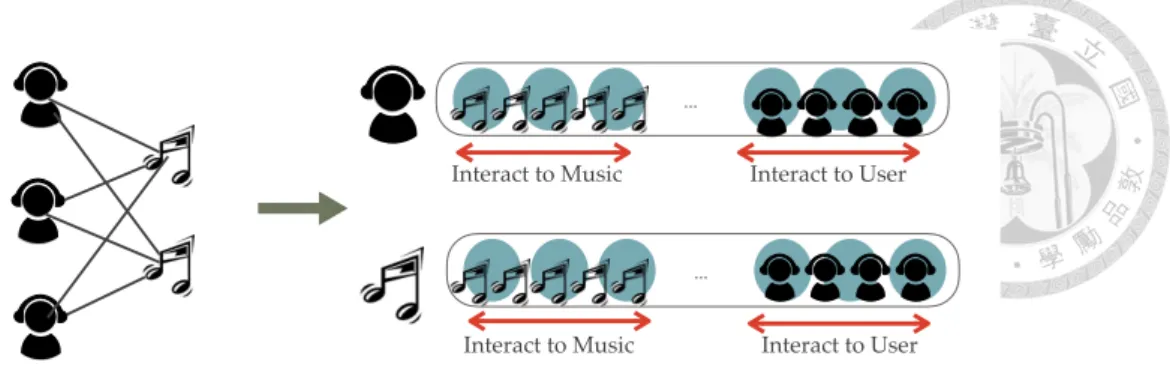
Figure 1.3: The goal of field-aware network embedding.
To address the imbalance problem, we proposed a field-aware network embedding model, which can independently learn the distinct kinds of vertex interactions based on the vertex fields. The proposed model learns multi-representation for each field, which implies the vertex position in latent space corresponding field, like the demonstration in figure 1.3. In fact, modeling the variant types interactions has been recognized as a useful method in factorization-based models [16, 12], but the presented solution is not directly applicable to the existing network embedding models. Hence, we propose the field-aware embedding providing a more suitable solutions to the network embedding models by con- sidering the similar concepts.
Our major contributions are as follows:
• A field-aware network embedding model is proposed to embed variant types of interactions into the learned representations from a heterogeneous network.
• Due to that different interaction types are modeled separately, it alleviates the im- balance training issue.
• We conduct the experiments on three public datasets. The proposed model can out- perform than general network embedding method which do not consider the inter- action types.
Chapter 2
Related Works
Our work is mainly involved with the three parts, 1) the concept of field-aware, 2) the technique of network embedding algorithms and 3) the work related to heterogeneous networks.
2.1 The idea of field-aware
FFM [12] used the field-aware concept in factorization machine, the model performs well in Click Through Rate (CTR) prediction problem. The factorization machine esti- mates the effect of feature conjunction by factorizing it into a product of two latent vec- tors. Therefore, every feature has only one latent vector to learn the latent effect with any other features. However, when it comes to 3 or more fields, the latent effect from different fields may be different. FFM tackles the problem with the idea of field-aware, makes the model learns different depending on the field of other features. In the proposed model, we use the similar concept of field-aware to deal with the incomparable problem in heterogeneous networks embedding.
2.2 Network Embedding algorithms
Network embedding becomes popular for its efficiency and effectiveness. The learned low-dimensional vector from network structure is useful for many machine learning appli- cations, such as link prediction, classification, ..., etc. One main reason is that the learned representations greatly keeps the vertices relations and the network structure in the given network. Moreover, these representations are vector-computable, which keeps the vertices similarity information.
In the literature, there are a number of network embedding models have been proposed to learn the feature representation. Graph factorization [2, 3] uses the matrix factorization to model the interactions among the objects in a graph network so that the factorized la- tent vectors represents the learned representations. GraRep [4] focus on the high-order relations and combine it with singular value decomposition (SVD) to construct multi- step learned representations. DeepWalk [15] exploits the random walk to sample the data relations from the network and use the skip-gram model to learn the representations.
Node2Vec [8] learns high-order information based on the estimate the transition prob- ability of neighborhoods. LINE [20] is the first attempt to preserve both the local and global network structure in the representations. In summary, the core of building a net- work embedding model is to determine which vertices are considered to be similar and which vertices are considered to be dissimilar. Given a relation network, the proposed model adopts the two criteria 1) the vertices which are connected to each other are similar to each other and 2) the vertices which share the common neighbor vertices are similar to each other.
In addition, some network embedding models try to going deep. SDNE [21] follows the same concepts in LINE and adopts a semi-supervised deep learning model. HNE [5]
uses transfer learning to combine the several different networks together. However, most of these models are supervised learning algorithms. They optimize the goals depending on specific task, while our work focuses on the unsupervised learning solution to an arbitrary network.
2.3 Heterogeneous Networks
Most of the real world datasets are heterogeneous networks, and they contain at least two different data types, such as the social network (user-content), the purchase networks(user- item), the citation networks (author-paper-conference), the language networks (document- word-label). Therefore, learning the relations in heterogeneous networks is an attracting research topic.
There also exists several researches using heterogeneous networks. [13] pre-defines some rules to capture the information in paper citation networks. [9] re-defines the weights among different types and finds out 16 relationships in online music streaming services (MSS). [14] tries to discover meta-path automatically in knowledge-based problem. These kinds of defined meta-path method [23, 17] are not only improving the performance in machine problem but also interpretable. However, such rule-based solutions require spe- cific background/domain knowledge to enable the learning process.
Some researches [5, 18] learn only one latent vector at a time, than to project the latent vectors into the same latent space. [1] proposes a statistical model called nCRF to combine the topic model for social media (Tweets) with geographical location. Although these kinds of method provide the representations cross networks, they ignore the relation of different types during the optimization/learning steps.
[11] reconstructs the heterogeneous network into one homogeneous network. [19]
divides the text heterogeneous network into three network, because the learned represen- tations from previous network embedding algorithms are incomparable. However, the proposed method is not suitable for general case. In this paper, we proposed the general- purpose field-aware network embedding algorithm to model different relationships in het- erogeneous network and provide multi-representations for each vertices.
Chapter 3 Methodology
3.1 Problem Definition
We define a graph G = (V, E), where V contains a set of vertices and E contains a set of edges. Each vertex represents an instance in the dataset and belongs to a certain field f . Each edge presents the relation between two certain vertices. In order to increase the information from a spare connection dataset, we consider that the vertices which can be reached within a short walk steps are all the neighborhood of the starting vertex v, denoted as N eighbor(v). This can help capture the idea that similar vertices usually share common neighbor vertices.
The task of an embedding model is to learn the mapping function Φ: V → Rd, where d represents the dimensions and d ≪ |V | which is low-dimensional. In the proposed field-aware network embedding, we model the representation from the two perspectives:
1. Φ1 for modeling the first-order relations, which means the vertices which are con- nected to each other shall be similar to each other
2. Φ2 for modeling the second-order relations, which means the vertices which share the common neighbor vertices shall be similar to each other.
The concept of the first-order and second-order relations are the same in [20]. It defines that each vertex plays two roles: the vertex “itself” and a specific “context” of other ver-
tices. In this work, Φ1 is for the representation treated as vertex itself, while Φ2 is the representation treated as a specific context.
Note that the direct learning of the second-order relations may suffer from the relation imbalance issue [5, 6]. To tackle with both the interaction types and relation imbalance issues, we further model Φ2with distinct mapping functions when the vertex interacts with different fields. That is, a vertex vi is mapped by Φ2f
vj(vi) when it interacts with a vertex vj with field fvj.
3.2 Field-aware embedding structure
Figure 3.1 (left) is an example of input network with 5 vertices. The user symbols belong to the user type, the others belong to the track type. The proposed field-aware embedding framework can be represented by a single-layer neural network, where the input and output are a vector representation, as the shown in Figure 3.1 (right). In this section, we first discuss why the solution of [12] is not applicable to the existing network embedding models, and then to present our proposed solution.
Φ U Φ ′
U2 U1
T5 T4
U3
Φ T Φ T Φ U Φ U
0 0 0 1 0
1 0 0 0 0
0 0 0 0 1
Φ T Φ U
Φ T Φ U
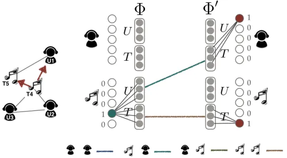
Figure 3.1: The diagram of Multi-Representation Multi-Context
Left: Example network. Right: The model input and context output for pairs in (T4, U1) and (T4, T5)
To directly use the solution of [12], it is an idea to modify the modeling structure to be a “Multi-Representation Multi-Context” form like the Figure 3.1 (right). By applying this to the second-order relation embedding, each vertex learns the latent effect from one of other features for both the vertex input and the context output. For instance, for the pairs in (T4, U1) and (T4, T5) in the example network, we estimate the conditional proba- bility p(U1|T4) and p(T5|T4) respectively. Consequently, we can observe that there are a total of 4 relationships: user(U)-user(U), user(T)-track(U), track(U)-user(T) and track(T)- track(T). The user compresses the information of user(U) and track(U), and the track com- presses the user(T) and track(T), so they are not comparable to each other. In summary, since they compress the information from different latent spaces, the structure of multi- representation multi-context is fail to tackle the incomparable problem.
Φ U Φ ′
U2 U1
T5 T4
U3
Φ T Φ T Φ U Φ U
0 0 0 1 0
1 0 0 0 0
0 0 0 0 1
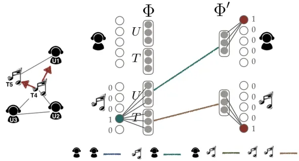
Figure 3.2: The diagram of Multi-Representation Single-Context
Left: Example network. Right: The model input and context output for pairs in (T4, U1) and (T4, T5)
To avoid learning the information from wrong space, we propose another proper mod- eling structure: “Multi-Representation Single-Context”. Figure 3.2 demonstrates the model of multi-representation single-context. We map the context output with only one out- put vector. Consequently, we can observe that the 4 relationships become: user(U)-user,
user(T)-track, track(U)-user and track(T)-track. Therefore, the user compresses the infor- mation of user and track, and the track compresses the user and track as well, so they are comparable to each other. Moreover, the information of the interaction types are sepa- rately stored in distinct representations (i.e. user/item(U) and user/item(T)).
3.3 Model Description
The embedding model is an attempt to capture the relations among the vertices in a network. Following the embedding learning criteria that the vertices which share common neighbor vertices are supposed to have similar representations, we define the demand sim- ilarity probability of an observed pair (vi, vj) by follows:
p(vj|vi) =
1 if vj ∈ Neighbors(vi) 0 otherwise
. (3.1)
To obtain the proper vertex representations in the proposed field-aware embedding model, the first-order relations are modeled the same as the previous work [20] by:
ˆ
p(vj|vi) = σ(Φ1(vi)· Φ1(vj)), (3.2)
where σ is the sigmoid function that re-scales the measured distance from 0 to 1. The directly connected are mapped with similar representations.
As to the second-order relations, we map each vertex by the mapping functions Φ2for the vertex mapping and Φ2′ for the neighbor mapping. The preceding defined relations can be modeled by measuring the representations distance:
ˆ
p(vj|vi) = σ(Φ2(vi)· Φ2′(vj)). (3.3)
Consequently, the vertices which share common neighbor vertices will receive closed rep-
resentations which fit the requirements.
To integrate the filed-aware concept with second-order relations learning, we propose to map a vertex with multiple representations based on the interaction type, called multi- representations single context. The interaction type is depended on the interaction vertex.
For a pair (vi, vj), the vertex vi is mapped according the type of the neighbor vertex vj:
ˆ
p(vj|vi) = σ(Φ2f
vj(vi)· Φ2′(vj)). (3.4)
To fit the defined requirements in Equation 3.2 and 3.4, the task becomes to minimize the gap between the ground truth p(vj|vi) and the estimation function ˆp(vj|vi). The final objective function is equivalent to minimize following distance function:
O = ∑
(vi,vj)∈S
d(p(vˆ j|vi), ˆp(vj|vi)), (3.5)
where S is the set of sampling pair.
3.4 Model Optimization
We use the KL-divergence to minimize the distance of the ground truth and the esti- mation function. By replacing ˆd(·, ·) with KL-divergence and omitting some constants, we have:
O = ∑
(vi,vj)∈S
dˆKL(p(vj|vi), ˆp(vj|vi))
≈ ∑
(vi,vj)∈Spos
− log ˆp(vj|vi) + ∑
(vi,vj)∈Sneg
log ˆp(vj|vi).
(3.6)
There are two cases in the derivative objective function. The former one is for mod- eling positive pairs in Spos and the latter one is for modeling negative pairs in Sneg. We adopt the stochastic gradient algorithm (SGD) method to optimize the objective function.
In details, it calculates the partial derivative of∂O∂⃗v when updates the representation of v in
a sampling pair. The derivation of vi in the positive case is:
∂ − log ˆp(vj|vi)
∂ ⃗vi =−(1 − σ(⃗vi · ⃗vj))· vj (3.7)
The derivation of vi in the negative case is:
∂ log ˆp(vj|vi)
∂ ⃗vi = σ(⃗vi· ⃗vj)· vj (3.8)
Note that vj is updated in a similar way. By iteratively updating the representations ac- cording to the sampling pairs in Spos and Sneg. The final obtained representations are approximated towards the demand ground truth. Algorithm 1 shows the whole learning procedure. In the following experiments, we update each Φ by the batch SGD.
Algorithm 1: Field-Aware Network Embedding (FNE)
Input: Network Graph: G(V, E) with the Field Set F , Learning Rate: α, Sampling Times: t
1 for v ∈ V do
2 Initialize the representations: Φ1(v), Φ2′(v)
3 for f ∈ F do
4 Initialize the representations: Φ2f(v)
5 for counter∈ {1, ..., t} do
6 for (vi, vj)∈ Spos do
7 Φ = Φ− α × (−(1 − σ(⃗vi· ⃗vj))· vj)
8 for (vi, vj)∈ Snegdo
9 Φ = Φ− α × σ(⃗vi· ⃗vj)· vj
Output: Vertex representations Φ1 and Φ2f for every f
Chapter 4 Experiments
We conduct the experiments on three public real-world datasets with three variant ma- chine learning applications, including network reconstruction, multi-label classification and item recommendations.
4.1 Dataset
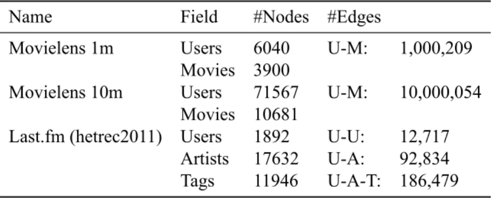
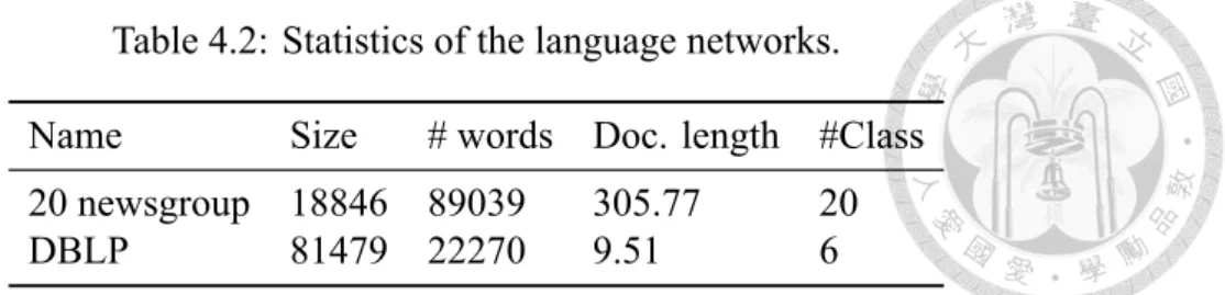
The conducted experiments include two kinds of network datasets: (1) Network datasets including movielens [10] and last.fm datasets. The statistics is shown in Table 4.1. (2) Language network datasets including 20 newsgroup and DBLP [22]. The summary of datasets in shown in Table 4.2.
• Movielens1: We use two movielens datasets 1m and 10m. Movielens datasets con- tain basic user information, such as user age, gender. There are 18 movie genres as movie information, for each movie, it belongs to at least one genre. The rating score of a user given a movie is range from 1 to 5. We only use the rating higher than 3 stars as the positive relations for the following experiment settings. Based on the rating scores, we construct a bipartite network containing the user-movie relation.
1https://grouplens.org/datasets/movielens/
• Last.fm2: Last.fm is a social music website3. The website provides a function that users are able to tag the tags to the artists. In this paper, we use the last.fm dataset provided by hetrec2011. There are three fields in this network, the user, the artist and the tag. In this dataset, there are 1,892 users, 17,632 artists and 11,946 tags. The total edges in this network is 31,470. Based on user-artist and user social datasets, we construct a network contains user-artist relation and user-user relation.
• 20 Newsgroups4: The 20 Newsgroups data set is a collection of approximately 20,000 newsgroup documents, partitioned (nearly) evenly across 20 different news- groups.
• DBLP5: Dblp, which contains titles of papers from the computer science bibliog- raphy. Follow the same setting in [19], we choose six diverse research fields for classification including “database”, “artificial intelligence”, “hardware”, “system”,
“programming languages”, and “theory”. For each field, we select representative conferences and collect the papers published in the selected conferences as the la- beled documents.
We build the user-item network based the user preference, and it is a heterogeneous net- work with two vertex types.
Table 4.1: Statistics of the real-world network datasets.
Name Field #Nodes #Edges
Movielens 1m Users 6040 U-M: 1,000,209
Movies 3900
Movielens 10m Users 71567 U-M: 10,000,054 Movies 10681
Last.fm (hetrec2011) Users 1892 U-U: 12,717 Artists 17632 U-A: 92,834 Tags 11946 U-A-T: 186,479
2https://grouplens.org/datasets/hetrec-2011/
3https://www.last.fm/
4http://qwone.com/ jason/20Newsgroups/
5http://arnetminer.org/billboard/citation
Table 4.2: Statistics of the language networks.
Name Size # words Doc. length #Class 20 newsgroup 18846 89039 305.77 20
DBLP 81479 22270 9.51 6
4.2 Compared Algorithms
We use FNE as the abbreviation of the proposed filed-aware network embedding model, and compares the FNE model with several existing graph embedding methods:
• DeepWalk [15] is a method that learns the representation of social networks using a sequence of truncated random walks. The truncated random walks, random path, contain high-order information, then using skip-gram to optimize the problem.
• LINE [20] learns vertex representations with two defined the skip-gram objective functions to capture the both local and global information. The defined loss func- tions can preserve the first-order or second-order proximity separately.
• GraRep [4] captures successive k-step information through random walk, then fac- torizing the transition matrix with SVD.
• PTE [19] proposed a framework which divide a text heterogeneous network into small networks, learns one relation at a time.
4.3 Evaluation Metrics
In this paper, we conduct 3 machine learning problem to evaluate model performance.
We use following metric to evaluate different applications.
• Recall (also known as sensitivity) is the fraction of relevant instances that have been retrieved over total relevant instances, which is computed as follow:
recall = #retrieved relevant documents
(4.1)
• MAP (mean averaged precision) for a set of queries is the mean of the average precision scores for each query. The formula is showed as follow:
M AP =
∑Q
q=1Avg Precision( q )
#Q (4.2)
• Macro-F1 is a metric which gives equal weight to each class. It is defined as fol- lows:
M acro− F 1 =
∑
A∈CF 1(A)
|C| , (4.3)
where F 1(A) is the F1-measure for the label A and C is the overall label set.
• Micro-F1 is a metric which gives equal weight to each instance. It is defined as follows:
P recision =
∑
A∈CT P (A)
∑
A∈CT P (A) + F P (A), Recall =
∑
A∈CT P (A)
∑
A∈CT P (A) + F N (A) (4.4) M icro− F 1 = 2× Precision × Recall
Precision + Recall (4.5)
4.4 Parameter Settings
Our experiments were conducted based on the same criteria. For both movielens rating networks and lastfm tagging network, the dimension is set as 200 by default. In LINE model, 100 dimensions for first-order proximity and second-order proximity. In FNE, we use same ratio for first-order and fields-aware multi-representations for each fields, that is, we set dimensions as 66 for each. Other default settings include: the number of window size win = 5, walk length t = 64, walks per vertex = 28 for DeepWalk; the number of negative samples K = 5, total number of samples T = 10 billion for LINE. Same settings in FNE: the number of negative samples K = 5 and total number of samples T = 10 billions.
As to language networks, we set minimum count as 0, window size as 5 for PTE to construct a word-word network. Then combines the word-word network, word-document
network and word-label network to compose a text heterogeneous network. As to learn- ing feature representations, we use the same settings for both FNE and PTE: number of samples(T) = 10 billion, negative samples K = 5 and vertex representation D = 200.
4.5 Experiment Results
4.5.1 Network Reconstruction
FNE
UserMovie
LINE
UserMovie
DeepWalk
UserMovie
GraRep
UserMovie
Figure 4.1: The 2-dimensional representations obtained from each baseline model on Movielens-1m.
Network reconstruction is a task to test whether the learned representations are able to reflect the connected relations of the original network. Figure 4.1 is the visualization of the movie rating network (movielens 1m). Both users and movies are mapped to the 2-D space using the t-SNE6package with learned embeddings as input. From the visualization results, the vertices in FNE is keeps together, however the others are mapped into the separated areas, because that the vertex representations from other models is learned from different latent spaces. Although bringing the information from high-order might ease up the problem, the learned representations are still affected by the imbalanced ratio of vertex types. This indicates that the existing network embedding models cannot perform well in network reconstruction for certain heterogeneous networks such as the examined user-item network.
In addition to the visualization result, we evaluate the performance of the network reconstruction task by following procedures: (1) Use 80% data as training data, 20% as
6http://scikit-learn.org/stable/modules/generated/sklearn.manifold.TSNE.html
Table 4.3: The network reconstruction results in Movielens datasets (1m & 10m)
Dataset Movielens-1M Movielens-10M
Model FNE LINE GraRep DeepWalk FNE LINE GraRep DeepWalk
TopN N = 10
Recall@10 0.2099 0.0007 0.0167 0.0068 0.1251 0.0217 - 0.0192
MAP@10 0.1081 0.0001 0.0058 0.0019 0.0674 0.0076 - 0.0066
TopN N = 20
Recall@20 0.2192 0.0008 0.017742 0.0094 0.1134 0.0216 - 0.0185
MAP@20 0.0894 0.0001 0.0043 0.0017 0.0483 0.0052 - 0.0044
TopN N=30
Recall@30 0.2407 0.0011 0.0186 0.0129 0.1116 0.0221 - 0.0186
MAP@30 0.0852 0.0001 0.0037 0.0017 0.0413 0.0042 - 0.0035
Table 4.4: The network reconstruction results in Last.fm
Model FNE LINE GraRep DeepWalk
TopN N = 10
Recall@10 0.0354 0.0357 0.0141 0.0355 MAP@10 0.0178 0.0191 0.0084 0.0176
TopN N = 20
Recall@20 0.0413 0.0397 0.0151 0.0410 MAP@20 0.0151 0.0162 0.0076 0.0153
TopN N=30
Recall@30 0.0521 0.0476 0.0169 0.0506 MAP@30 0.0159 0.0168 0.0077 0.0161
testing data. (2) Construct a network from training data and learned vertex representations.
(3) Evaluate performance by given one vertex, evaluate the recall@N and MAP@N of retrieved connected edges. We repeat the procedure 5 times and report the average result.
The performance is showed as table 4.3 and table 4.4. In movielens networks, our model outperforms all compared methods. However in lastfm network, our model obtains similar performance of LINE and DeepWalk because the dataset provides user-user connections, which alleviates the connection imbalance problem. Please note that the GraRep model is unable to run on Movielens-10M graph with limited memory, so we do not report the result.
Table 4.5: The multi-label classification results in Movielens datasets (1m & 10m).
Dataset Movielens-1M Movielens-10M
Model FNE LINE GraRep DeepWalk FNE LINE GraRep DeepWalk
Train Ratio 10%
Micro-F1 0.7513 0.7001 0.6817 0.7183 0.6661 0.6179 - 0.5578 Macro-F1 0.6589 0.5544 0.4237 0.6123 0.5435 0.4917 - 0.4277
Train Ratio 30%
Micro-F1 0.8087 0.7728 0.7363 0.7568 0.6934 0.6581 - 0.6334 Macro-F1 0.7722 0.6956 0.5639 0.7008 0.6934 0.6581 - 0.6334
Train Ratio 50%
Micro-F1 0.8268 0.7984 0.7543 0.7763 0.6934 0.6581 - 0.6334 Macro-F1 0.8126 0.7439 0.6161 0.7338 0.6934 0.6581 - 0.6334
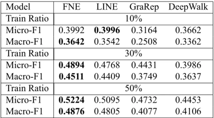
Table 4.6: The multi-label classification results in Last.fm.
Model FNE LINE GraRep DeepWalk
Train Ratio 10%
Micro-F1 0.3992 0.3996 0.3164 0.3662 Macro-F1 0.3642 0.3542 0.2508 0.3362
Train Ratio 30%
Micro-F1 0.4894 0.4768 0.4431 0.3986 Macro-F1 0.4511 0.4409 0.3749 0.3637
Train Ratio 50%
Micro-F1 0.5224 0.5095 0.4732 0.4453 Macro-F1 0.4876 0.4805 0.4077 0.4106
4.5.2 Multi-label Classification
This task is to classify the items attributes based on the learned representations. For movielens dataset, we use movie genre as the labels; for last.fm dataset, we use the top 20 artist tags as the labels. Similar to [20, 19], for each class, we train a one-vs-rest logistic regression classifier using the LibLinear package [7]. We use Macro-F1 and Micro-F1 as evaluation metrics. The results are averaged over 5 different runs by sampling different training data. The performance is shown in Table 4.5 and Table 4.6. Again, the GraRep model is unable to run on Movielens-10M graph with limited memory, so we do not report the result. As the table shows, the FNE model outperforms the other models on movielens network. As to lastfm dataset, our model is slightly to lose LINE in train ratio at 10%.
However, as the train ratio increase, our model get better results.
Table 4.7: The item recommendation results in Movielens datasets (1m & 10m).
Dataset Movielens-1M Movielens-10M
Model FNE LINE GraRep DeepWalk FNE LINE GraRep DeepWalk
TopN N = 10
Recall@10 0.2099 0.0007 0.0167 0.0068 0.1809 0.0042 - 0.0036
MAP@10 0.1081 0.0001 0.0058 0.0019 0.0954 0.0014 - 0.0011
TopN N = 20
Recall@20 0.2192 0.0008 0.0177 0.0094 0.2199 0.0047 - 0.0040
MAP@20 0.0894 0.0001 0.0043 0.0017 0.0938 0.0010 - 0.0008
TopN N=30
Recall@30 0.2407 0.0011 0.0186 0.0129 0.2549 0.0054 - 0.0045
MAP@30 0.0852 0.0001 0.0037 0.0017 0.0966 0.0008 - 0.0007
Table 4.8: The item recommendation results in Last.fm.
Model FNE LINE GraRep DeepWalk
TopN N = 10
Recall@10 0.1152 0.0398 0.0037 0.0702 MAP@10 0.0563 0.0186 0.0014 0.0373
TopN N = 20
Recall@20 0.1437 0.0448 0.0050 0.0758 MAP@20 0.0522 0.0157 0.0012 0.0314
TopN N=30
Recall@30 0.1799 0.0573 0.0064 0.0928 MAP@30 0.0565 0.0167 0.0012 0.0330
4.5.3 Link Prediction / Item Recommendations
Link prediction is also called item recommendations in these kind of bipartite net- works. Follow the similar procedure in networks reconstruction, (1) we randomly hide a portion of the existing links and train on the remain network. (2) For each user-vertex, we use the learned representation to predict the unobserved links. From the retrieved items, we evaluate the performance by recall@N and MAP@N. Table 4.7 and Table 4.8 lists the scores of the MAP and recall. The results are consistent with the network reconstruction task that the existing network embedding models cannot perform well in neighborhood predictions, while FNE solves the problem.
Table 4.9: The documents classification results on 20 newsgroup and DBLP datasets.
Dataset 20 newsgroup DBLP
Metric Macro-F1 Micro-F1 Macro-F1 Micro-F1
FNE 0.4888 0.6435 0.6849 0.7570
PTE 0.4518 0.6147 0.6760 0.7433
4.5.4 Documents Classification
The document classification task is conducted on text heterogeneous networks, which contains documents, label of documents, and words in documents. This is a special case of heterogeneous networks due to the edges between vertexs is link by people heuristic.
Follow the settings in [19], we construct a heterogeneous networks contains three fields, such as words, documents, labels. The evaluate procedure is as follows: (1) Obtain word embeddings from construct language network. (2) Take the average of the word vector rep- resentations in that document as document representations. (3) Train a one-vs-rest logistic regression classifier using package (LibLinear [7]). Table 4.9 reports the performance of document classification. From the table, FNE outperforms PTE on both datasets. The result proves that our model can learns better word embeddings without preprocessing the network form.
4.5.5 Experiment Results Summary
Our model focuses on dealing with the incomparable problem in heterogeneous net- work embedding by modeling different interaction separately. The above experiment re- sults prove the effectiveness of proposed method. Moreover, our model much improves the performance on cross-field problems, such as item recommendation, network recon- struction on bipartite network. The reason is that different type of node representations can be comparable. As to machine learning applications such as classification which only focusing on one type representations, our model can obtain the same or better results than other baseline methods.
Chapter 5 Discussion
In this chapter, we construct several experiment to examine different factor affected the model, such as model parameters and the dimension of fields.
5.1 Parameter Sensitive
In this section, we analyze the model performance respect with parameter sensitivity.
5.1.1 Performance w.r.t. #Samples
The time complexity of our model is O(tsd), where t is the number of iteration, s is the number of negative samples and d is the dimension of representations. The number of s and d are usually smaller than t, therefore, the converging performance of model is mainly affect by iterations. Figure 5.1 shows the results of two machine learning applications w.r.t. #samples on Movielens-1m datasets. We can know that our model is converge at early stages.
5.1.2 Performance w.r.t. Dimension
The field-aware network embedding algorithm provides multi-representations for each fields. As a result, the dimension can be divide into several parts, vector for first-order
0 500 1000 1500 2000 2500 3000 3500 0.065
0.070 0.075 0.080 0.085 0.090 0.095 0.100 0.105 0.110
(a) The link prediction result w.r.t. #samples.
0 500 1000 1500 2000 2500 3000 3500
0.55 0.60 0.65 0.70 0.75 0.80 0.85 0.90
(b) The multi-label classification result w.r.t.
#samples.
Figure 5.1: The performance of two machine learning applications w.r.t. #samples on Movielens-1m datasets.
used to capture direct relations in network; vector for f ield1 used to capture the latent from f ield1; f ield2 used to capture the latent from f ield2, ..., etc. As the number of field increase, the vertex representations would be divide into many small segments. If the dimension is too small, the representations is unable to represents the vertex well.
Figure 5.2 shows the performance of multi-label classification respect with the number of dimension. Although when the dimension is small, our model is fail to surpass other models, as we gradually increase the dimension of representations, our model begins to outperform other methods.
5.1.3 Performance w.r.t. Network Sparsity
We investigate how the sparsity of the networks affects the models. Figure 5.3 shows the results w.r.t. the degrees of the vertices on movielens 1m and 10m datasets. We cate- gorize the vertices into different groups according to their degrees including (0, 1], [2, 4], [5, 8], [9, 16], [17, 32], [33,∞) and then evaluate the performance of vertices in different groups. Overall, the performance of different models increases when the degrees of the
40 60 80 100 120 140 160 180 200 Dimension
0.75 0.76 0.77 0.78 0.79 0.80 0.81 0.82 0.83
Micro-F1
FNE LINE DeepWalk
(a) ML-1m
40 60 80 100 120 140 160 180 200
Dimension 0.59
0.60 0.61 0.62 0.63 0.64 0.65 0.66 0.67
Macro-F1
FNE LINE DeepWalk
(b) ML-10m
40 60 80 100 120 140 160 180 200
Dimension 0.42
0.44 0.46 0.48 0.50 0.52 0.54
Micro-F1
FNE LINE DeepWalk
(c) Last.fm Figure 5.2: The multi-label classification result w.r.t. Dimension on three datasets.
1 2 3 4 5 6
degree group 0.50
0.55 0.60 0.65 0.70 0.75 0.80 0.85
Macro-F1
FNE LINE grarep DeepWalk
(a) ML-1m
1 2 3 4 5 6
degree group 0.3
0.4 0.5 0.6 0.7 0.8
Micro-F1
FNE LINE DeepWalk
(b) ML-10m
1 2 3 4 5 6
degree group 0.0
0.1 0.2 0.3 0.4 0.5 0.6 0.7 0.8
Micro-F1
FNE LINE grarep DeepWalk
(c) Lastfm
Figure 5.3: The multi-label classification result w.r.t. Degree of vertices on three datasets.
vertices increase. The LINE outperforms FNE in the first group because that that LINE optimizes only the directly connected vertices and does not add the information from high- order. The performance in ML-10m is more stable than ML-1m, because the amount of data records. Our model obtains the same or better results than LINE in ML-10m. We can also see that our model outperforms DeepWalk and GraRep in all the groups.
5.2 Dimension of Fields
In this section, we investigate how the dimension of different fields affect the perfor- mance. We set user dimension range from 0 to 100, item dimension range from 0 to 100, then conduct two machine applications (multi-label classification and link prediction) to evaluate the performance. Figure 5.4 shows the performance of two machine applications
0 10 20 30 40 50 60 70 80 90 100 Movie Dimension
100 90 80 70 60 50 40 30 20 10 0
User Dimension
0.770 0.775 0.780 0.785 0.790 0.795 0.800 0.805 0.810 0.815 0.820
(a) Multi-label Classification (Micro-F1)
0 10 20 30 40 50 60 70 80 90 100 Movie Dimension
100 90 80 70 60 50 40 30 20 10 0
User Dimension
0.000 0.003 0.006 0.009 0.012 0.015 0.018 0.021 0.024 0.027 0.030
(b) Link Prediction (MAP) Figure 5.4: The performance w.r.t User-Movie dimensions on ML-1m.
w.r.t different User-Movie dimension pair on Movielens 1m dataset. From two figures, we find that the dimension of movies as 20∼ 30 can obtain the best result, the dimension higher than this range might overfit the training data. On the other hand, the dimension need of user is range 40 ∼ 70 in multi-label classification task and 35 ∼ 80 in link pre- diction task. The most interesting is that we only use the learned movie representations to train a classifier in multi-label classification task, the model without user information get the worst performance. In link prediction task which needs both user-representations and movie-representations, the model without any information get the worst performance.
Chapter 6 Conclusion
In this paper, we propose a field-aware network embedding that models the rich it- eration information from heterogeneous network. The proposed model use the “Multi- Representation Single Context” structure which models the different types of interactions separately and generates low dimension vertices representations for each field. Our model not only can learns iteration from different type without pre-process network but also deal- ing with the incomparable problem of different type of nodes. Also, the structure of our model makes us able to set different field dimension which provides more flexibility and explanation of data.
The experimental results on various networks show that it is able to improve the rep- resentation capability of machine learning applications such as network reconstruction, multi-label classification and link prediction. Moreover, our model have much improve the performance of cross-field problem such as recommendation than other network em- bedding methods.
Bibliography
[1] A. Ahmed, L. Hong, and A. J. Smola. Hierarchical geographical modeling of user locations from social media posts. In Proceedings of the 22Nd International Con- ference on World Wide Web, WWW ’13, pages 25–36, New York, NY, USA, 2013.
ACM.
[2] A. Ahmed, N. Shervashidze, S. Narayanamurthy, V. Josifovski, and A. J. Smola.
Distributed large-scale natural graph factorization. In Proceedings of the 22Nd In- ternational Conference on World Wide Web, WWW ’13, pages 37–48, New York, NY, USA, 2013. ACM.
[3] M. Belkin and P. Niyogi. Laplacian eigenmaps for dimensionality reduction and data representation. Neural Comput., 15(6):1373–1396, June 2003.
[4] S. Cao, W. Lu, and Q. Xu. Grarep: Learning graph representations with global structural information. In Proceedings of the 24th ACM International on Conference on Information and Knowledge Management, CIKM ’15, pages 891–900, New York, NY, USA, 2015. ACM.
[5] S. Chang, W. Han, J. Tang, G.-J. Qi, C. C. Aggarwal, and T. S. Huang. Hetero- geneous network embedding via deep architectures. In Proceedings of the 21th ACM SIGKDD International Conference on Knowledge Discovery and Data Min- ing, KDD ’15, pages 119–128, New York, NY, USA, 2015. ACM.
[6] C.-M. Chen, M.-F. Tsai, Y.-C. Lin, and Y.-H. Yang. Query-based music recommen- dations via preference embedding. In Proceedings of the 10th ACM Conference
on Recommender Systems, RecSys ’16, pages 79–82, New York, NY, USA, 2016.
ACM.
[7] R.-E. Fan, K.-W. Chang, C.-J. Hsieh, X.-R. Wang, and C.-J. Lin. LIBLINEAR:
A library for large linear classification. Journal of Machine Learning Research, 9:1871–1874, 2008.
[8] A. Grover and J. Leskovec. Node2vec: Scalable feature learning for networks. In Proceedings of the 22Nd ACM SIGKDD International Conference on Knowledge Discovery and Data Mining, KDD ’16, pages 855–864, New York, NY, USA, 2016.
ACM.
[9] C. Guo and X. Liu. Automatic feature generation on heterogeneous graph for music recommendation. In Proceedings of the 38th International ACM SIGIR Conference on Research and Development in Information Retrieval, SIGIR ’15, pages 807–810, New York, NY, USA, 2015. ACM.
[10] F. M. Harper and J. A. Konstan. The movielens datasets: History and context. ACM Trans. Interact. Intell. Syst., 5(4):19:1–19:19, Dec. 2015.
[11] Y. Jacob, L. Denoyer, and P. Gallinari. Learning latent representations of nodes for classifying in heterogeneous social networks. In Proceedings of the 7th ACM International Conference on Web Search and Data Mining, WSDM ’14, pages 373–
382, New York, NY, USA, 2014. ACM.
[12] Y. Juan, Y. Zhuang, W.-S. Chin, and C.-J. Lin. Field-aware factorization machines for ctr prediction. In Proceedings of the 10th ACM Conference on Recommender Systems, RecSys ’16, pages 43–50, New York, NY, USA, 2016. ACM.
[13] X. Liu, Y. Yu, C. Guo, and Y. Sun. Meta-path-based ranking with pseudo relevance feedback on heterogeneous graph for citation recommendation. In Proceedings of the 23rd ACM International Conference on Conference on Information and Knowledge Management, CIKM ’14, pages 121–130, New York, NY, USA, 2014. ACM.
[14] C. Meng, R. Cheng, S. Maniu, P. Senellart, and W. Zhang. Discovering meta-paths in large heterogeneous information networks. In Proceedings of the 24th International Conference on World Wide Web, WWW ’15, pages 754–764, Republic and Canton of Geneva, Switzerland, 2015. International World Wide Web Conferences Steering Committee.
[15] B. Perozzi, R. Al-Rfou, and S. Skiena. Deepwalk: Online learning of social repre- sentations. In Proceedings of the 20th ACM SIGKDD International Conference on Knowledge Discovery and Data Mining, KDD ’14, pages 701–710, New York, NY, USA, 2014. ACM.
[16] S. Rendle and L. Schmidt-Thieme. Pairwise interaction tensor factorization for per- sonalized tag recommendation. In Proceedings of the Third ACM International Con- ference on Web Search and Data Mining, WSDM ’10, pages 81–90, New York, NY, USA, 2010. ACM.
[17] Y. Sun, J. Han, C. C. Aggarwal, and N. V. Chawla. When will it happen?: Relation- ship prediction in heterogeneous information networks. In Proceedings of the Fifth ACM International Conference on Web Search and Data Mining, WSDM ’12, pages 663–672, New York, NY, USA, 2012. ACM.
[18] J. Tang, T. Lou, J. Kleinberg, and S. Wu. Transfer learning to infer social ties across heterogeneous networks. ACM Trans. Inf. Syst., 34(2):7:1–7:43, Apr. 2016.
[19] J. Tang, M. Qu, and Q. Mei. Pte: Predictive text embedding through large-scale het- erogeneous text networks. In Proceedings of the 21th ACM SIGKDD International Conference on Knowledge Discovery and Data Mining, KDD ’15, pages 1165–1174, New York, NY, USA, 2015. ACM.
[20] J. Tang, M. Qu, M. Wang, M. Zhang, J. Yan, and Q. Mei. Line: Large-scale infor- mation network embedding. In Proceedings of the 24th International Conference
on World Wide Web, WWW ’15, pages 1067–1077, Republic and Canton of Geneva, Switzerland, 2015. International World Wide Web Conferences Steering Committee.
[21] D. Wang, P. Cui, and W. Zhu. Structural deep network embedding. In Proceedings of the 22Nd ACM SIGKDD International Conference on Knowledge Discovery and Data Mining, KDD ’16, pages 1225–1234, New York, NY, USA, 2016. ACM.
[22] J. Yang and J. Leskovec. Defining and evaluating network communities based on ground-truth. In Proceedings of the ACM SIGKDD Workshop on Mining Data Se- mantics, MDS ’12, pages 3:1–3:8, New York, NY, USA, 2012. ACM.
[23] X. Yu, X. Ren, Y. Sun, Q. Gu, B. Sturt, U. Khandelwal, B. Norick, and J. Han. Per- sonalized entity recommendation: A heterogeneous information network approach.
In Proceedings of the 7th ACM International Conference on Web Search and Data Mining, WSDM ’14, pages 283–292, New York, NY, USA, 2014. ACM.