張量網路演算法對Thirring 模型在一維無限長格點之研究

國立臺灣大學理學院物理學系 碩士論文

Department of Physics College of Science

National Taiwan University Master Thesis

張量網路演算法對 Thirring 模型在一維無限長格點之研究 Tensor Network Studies of Thirring Model on a One-dimensional

Infinite-size Lattice

洪浩迪 Hao-Ti Hung

指導教授：高英哲博士 Advisor: Ying-Jer Kao, Ph.D.

中華民國 107 年 6 月

June, 2018

致謝

碩士班兩年，回想起來真的很快。首先我要感謝我的指導教授高英 哲老師兩年來的指導，想當初進來時我說我想要做演算法應用在物理 模型上，果然真的讓我做了演算法，很幸運的，雖然一路上碰到一大 堆的問題，許許多多問題在我們討論之後都被一一解決了，幾乎可以 說是很順利的完成演算法。模型的部分，非常感謝林及仁教授在場論 模型這方面的指導。實驗室的許多學長姊都非常的熱心，我要感謝林 育平學長，在我剛進來時我幾乎全部的問題都問他，他都抽空幫我解 決，如果不是他的話我學習應該沒那麼順利。再來是周昀萱學長也常 常在程式方面教我許多技巧，讓我可以加速完成我的演算法，李致遠 學長、吳愷訢和趙凱文也常常幫我解決許多程式方面的問題，易德學 長也在我剛進來的時候給了不少的幫助，以及博士後 Adam 在英文方 面的幫助，博士後 Adil 也會給我一些研究方面的建議，還要感謝實驗 室許許多多的夥伴包含曾郁欽學長、高文瀚學長、鄭君筑學姊、鍾瑞 輝和顏敬哲在平常的閒聊，除了我們的團隊外我也要也感謝譚道璘以 及羅中佑學長給我許許多多的幫助，當然還有爸媽一路上的支持。最 後一定要感謝我的大學老師孫士傑老師的引薦。很開心可以來到這個 研究室做研究，讓我在數值方面的技巧更進一步。

doi:10.6342/NTU201802766

中文摘要

我們利用張量網路演算法研究 Thirring 模型。我們將模型離散化 後，找出 Thirring 模型哈密頓的自旋算符表示法並用矩陣作用算符表 示。

利用均勻矩陣乘積態的變分優化演算法去找出模型的基態解並調 查其相圖。然後利用時間相依變分原理來研究 Thirring 模型的動態演 化，特別是對於跨相變的動態演化特別有興趣。

關鍵字: 張量網路、矩陣乘積態、均勻矩陣乘積態的變分優化演算法、

時間相依變分原理、Tirring 模型、量子演化、動態相變

Abstract

We use tensor networks to study the Thirring model. We discretize the model onto the lattice, find the spin representation for the Hamilto- nian of the Thirring model and use the matrix product operator (MPO) to represent it.

Using the variational optimization algorithms for uniform Matrix Product State (VUMPS), we find the ground state of the model and investigate the phase diagram. Then, we use the time-dependent varia- tional principle algorithm (TDVP) to study the quench dynamics for the Thirring model, especially for what happens when quenching different phases.

Keywords: Tensor network (TN), matrix product state (MPS), varia- tional optimization algorithm for uniform matrix product state (VUMPS), time-dependent variational principle (TDVP), Thirring model, quantum quench, dynamical phase transition (DPT)

doi:10.6342/NTU201802766

Contents

口試委員會審定書 i

致謝 ii

中文摘要 iii

Abstract iv

1 Introduction 1

1.1 Overview . . . 1

2 Thirring Model 3 2.1 Spin Representation of the Thirring Model . . . 3

2.2 Chiral Condensate . . . 5

2.3 Mapping to the Classical 2D XY Model . . . 5

3 Tensor Network and Matrix Product state 6 3.1 Tensor Network and Tensor Diagram . . . 6

3.2 Matrix Product States . . . 7

3.3 Uniform Matrix Product States . . . 10

3.4 Expectation Values . . . 11

3.5 Gauge Degrees of Freedom, Canonical Form and Symmetric gauge . . 12

3.6 Geometric Series for Transfer Matrix . . . 16

3.7 Matrix Product Operator . . . 18

4 Variational Optimization Method for uniform Matrix Product State 20 4.1 Effective Hamiltonian . . . 20

4.2 VUMPS algorithm . . . 24

5 Time-Dependent Variational Principle Applied to Matrix Product State 27 5.1 Tangent Vector Space . . . 27

5.2 Gauge Fixing for Tangent Vector . . . 28

5.3 Projection Operator . . . 29

5.4 TDVP algorithm . . . 32

6 Result and Conclusion 34 6.1 Ground State of the Thirring Model . . . 34

6.2 TDVP Result . . . 40

7 Summary 43

Bibliography 44

Appendix

More Numerical Results 46

doi:10.6342/NTU201802766

List of Figures

3.1 Tensor network diagrams (a) a scalar, (b) a vector, (c) a matrix and

(d) a rank-3 tensor. . . 7

3.2 Tensor network diagram for Eqs. (3.1) and (3.2). . . 7

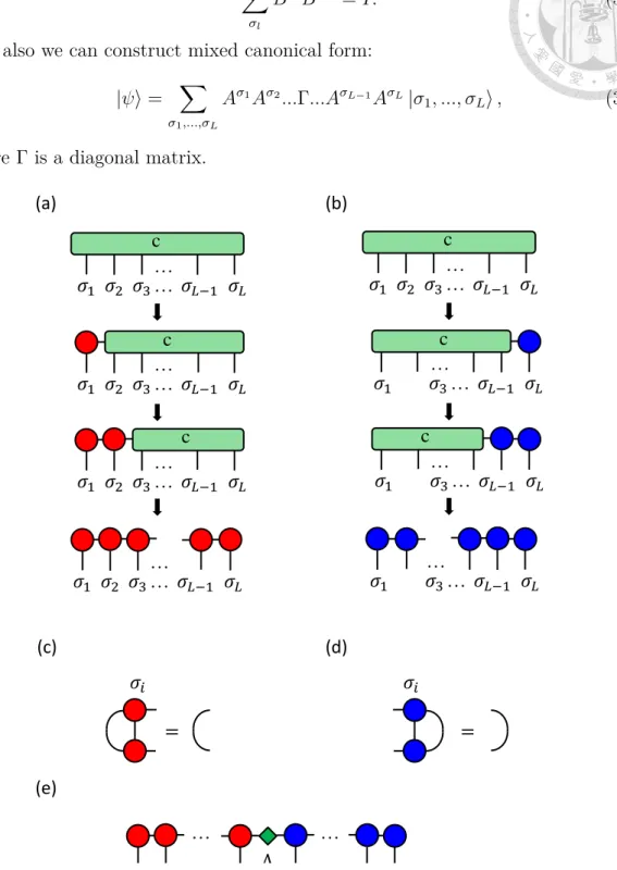
3.3 (a) Graphical representation of an iterative construction of left-canonical MPS from arbitrary quantum state by SVD. (b) Graphical repre- sentation of an iterative construction of right-canonical MPS from arbitrary quantum state by SVD. (c) The property of left canonical form. (d) The property of right canonical form. (e) Tensor network diagram of mixed canonical form. . . 9

3.4 Expectation value represented as a tensor network diagram. . . 11

3.5 (a) Use SVD to decompose tensor A. (b) (Λ,Γ) notation for uMPS. . 12

3.6 Check the property of the left canonical form. . . 14

4.1 (a) One-site effective Hamiltonian, (b) zero-site effective Hamiltonian (c) acting with tensor A_C on one-site effective Hamiltonian (d) acting with tensor C on zero-site effective Hamiltonian. . . . 21

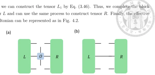
4.2 (a)one-site effective Hamiltonian (b)zero-site effective Hamiltonian . 24 4.3 Flow chart of VUMPS algorithm. . . 26

5.1 An illustration of the uMPS manifold and tangent space. The black dot represents the uMPS, ψ(A), and the tangent vector Φ(B; A) is a vector line on the tangent plane. . . 28

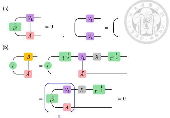
5.2 (a) The properties of V_L (b) The properties of tensor B . . . 29

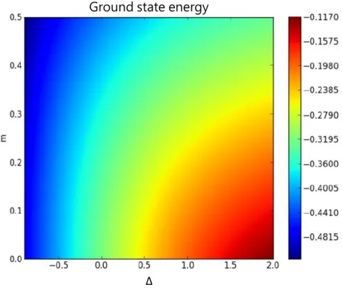
6.1 Energy density of the Thirring model. . . 34

6.2 Entanglement entropy of the Thirring model. . . 35

6.3 Chiral Condensate of the Thirring model. . . 35

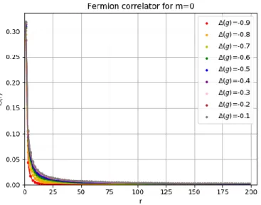
6.4 Fermion correlator for the massless case on a linear scale. . . 36

6.5 Fermion correlator for the massless case with a semi-log scale. . . 37

6.6 Fermion correlator for the massless case on a log-log scale. . . 37

6.7 Fermion correlator for the massive case on a linear scale for m=0.2. . 38

6.8 Fermion correlator for the massive case with a semi-log scale for m=0.2. 38 6.9 Fermion correlator for the massive case on a log-log scale for m=0.2. 39 6.10 ∆(g) near the transition. . . 39 6.11 The Thirring model evolving from (∆,m)=(-0.8, 0.2) to (∆,m)=(0.5,

0.2). . . 41 6.12 The Thirring model evolving from (∆,m)=(0.5, 0.2) to (∆,m)=(-0.8,

0.2). . . 41 A.1 The Thirring model evolving from (∆,m)=(0, 0) to (∆,m)=(0, 0.2). . 46 A.2 The Thirring model evolving from (∆,m)=(0.5, 0) to (∆,m)=(0.5, 0.2). 46 A.3 The Thirring model evolving from (∆,m)=(0, 0.2) to (∆,m)=(0, 0). . 47 A.4 The Thirring model evolving from (∆,m)=(0.5, 0.2) to (∆,m)=(0.5,

0). . . 47 A.5 The Thirring model evolving from (∆,m)=(-0.5, 0) to (∆,m)=(-0.5,

0.5). . . 48 A.6 The Thirring model evolving from (∆,m)=(0, 0) to (∆,m)=(0, 0.5). . 48 A.7 The Thirring model evolving from (∆,m)=(0.5, 0) to (∆,m)=(0.5, 0.5). 48 A.8 The Thirring model evolving from (∆,m)=(-0.5, 0.5) to (∆,m)=(-0.5,

0). . . 49 A.9 The Thirring model evolving from (∆,m)=(0, 0.5) to (∆,m)=(0, 0). . 49 A.10 The Thirring model evolving from (∆,m)=(0.5, 0.5) to (∆,m)=(0.5,

0). . . 50 A.11 The Thirring model evolving from (∆,m)=(0.5, 0.5) to (∆,m)=(0.5,

0.1). . . 50 A.12 The Thirring model evolving from (∆,m)=(-0.5, 0) to (∆,m)=(0.5, 0). 50 A.13 The Thirring model evolving from (∆,m)=(-0.8, 0) to (∆,m)=(0.5, 0). 51 A.14 The Thirring model evolving from (∆,m)=(0.5, 0.2) to (∆,m)=(0.2,

0.2). . . 51 A.15 The Thirring model evolving from (∆,m)=(0.5, 0.2) to (∆,m)=(0, 0.2). 51 A.16 The Thirring model evolving from (∆,m)=(0.5, 0.2) to (∆,m)=(-0.5,

0.2). . . 52 A.17 The Thirring model evolving from (∆,m)=(0.2, 0.2) to (∆,m)=(0.5,

0.2). . . 52 A.18 The Thirring model evolving from (∆,m)=(0, 0.2) to (∆,m)=(0.5, 0.2). 52 A.19 The Thirring model evolving from (∆,m)=(0, 0.2) to (∆,m)=(-0.8,

0.2). . . 53 A.20 The Thirring model evolving from (∆,m)=(-0.8, 0.2) to (∆,m)=(0,

0.2). . . 53

doi:10.6342/NTU201802766

Chapter 1 Introduction

1.1 Overview

Tensor network methods are taking a central role in modern quantum physics, especially in quantum many-body systems [1, 2]. In these methods, the quantum state is represented as a tensor network, which we call a tensor network state. There are several forms of tensor network states such as the matrix product state (MPS), which is a good representation of quantum states in 1D lattice systems, and the projected entangled pair state (PEPS), which is a representation of quantum states in 2D lattice systems. In this thesis, we will introduce the Thirring model on 1D infinite lattice in Chapter 2, and we use the so-called uniform matrix product state (uMPS) (or infinite MPS (iMPS)), which we will introduce in Chapter 3, to represent our quantum states.

There are several algorithms based on the tensor network methods for finding the ground state of system, such as density matrix renormalization group (DMRG) [3]

and infinite time-evolving block decimation (iTEBD) [4]. In this thesis, we use the variational optimization algorithm for uniform matrix product states (VUMPS) [5], which will be discussed in Chapter 4, to find the ground state of the Thirring model.

There are tensor network algorithms for simulating real-time evolution for many- body system on 1D lattices such as iTEBD or the time-dependent variational prin- ciple (TDVP) [6]. We extend the original TDVP algorithm using the idea of the infinite boundary conditions for MPS [7], and then we can use the matrix product operator (MPO) to do TDVP simulations (see Chapter 5).

A quantum quench is a protocol in which one prepares an eigenstate of one Hamiltonian, H₀, and then evolves dynamically in time under a different Hamilto- nian, H₁. We want to ask whether the Thirring model exists the dynamical phase transition [8]. We use the VUMPS algorithm to prepare the ground state of the

Thirring model with a given coupling constant (∆) and mass (m), which is also the eigenstate of Hamiltonian H₀, and do real-time evolution by using another parame- ters (∆^′,m^′) to investigate the quench dynamics of the Thirring model. We discuss our results in Chapter 6.

doi:10.6342/NTU201802766

Chapter 2

Thirring Model

2.1 Spin Representation of the Thirring Model

We want to discretize the massive Thirring model onto a 1D lattice¹. The massive Thirring model is a theory of Dirac fields in the (1+1)-dimensional spacetime with a current-current interaction; it is described by the action

S(ψ, ¯ψ) =

∫ d²x

[ψiγ¯ ^µ∂_µψ− m ¯ψψ− g

2( ¯ψγ^µψ)² ]

, (2.1)

where m denotes the mass and g is the coupling constant of the current-current interaction term ( ¯ψγ^µψ)². The canonical momentum is

Π = ∂L

∂ ˙ψ = ¯ψiγ₀ = iψ^†. (2.2) Thus, the Hamiltonian of the Thirring model becomes

H =

∫

dx (Π∂0ψ− L)

=

∫ dx

[ψiγ¯ ₀∂₀ψ− ¯ψiγ^µ∂_µψ + m ¯ψψ +g

2( ¯ψγ^µψ)² ]

=

∫ dx

[− ¯ψiγ¹∂₁ψ + m ¯ψψ +g

2( ¯ψγ^µψ)² ]

.

(2.3)

We choose the γ matrices as

γ₀ = σ₃, γ₁ = iσ₂, (2.4)

where σ_i are the Pauli matrices. We can see that the γ matrices will satisfy the Colifford algebra as{γµ, γ_ν} = 2gµν, where g_µν is the metric of the Minkowski space chosen as (1,-1).

1The part of the discussuin is based on Ref. [9].

In addition, we will use ϕ_u and ϕ_d to denote the up and down components of the field. Namely,

ψ = (ϕ_u

ϕ_d )

. (2.5)

Then, Eq. (2.3) becomes H =

∫

dx [−i(ψ^∗d∂₁ψ_u+ ψ_u^∗∂₁ψ_d) + m(ψ^∗_uψ_u− ψ^∗dψ_d) + 2g(ψ^∗_uψ_uψ^∗_dψ_d)] . (2.6) We want to discretize the Hamiltonian on a 1D infinite lattice with the lattice constant a and use “Kogut-Susskind fermions” [10], which put the up component ψ_u on the even sites and the down component ψ_d on the odd sites. Hence,

ψ_u → 1

√ac_2n, ψ_d→ 1

√ac_2n+1 (2.7)

and the differentials in space dimension are

∂₁ψ_u(x) =

√1

a(c_2n+1− c2n−1)

2a , ∂₁ψ_d(x) =

√1

a(c_2n+2− c2n)

2a . (2.8)

Then Eq. (2.6) becomes Hlattice =− i

2a

∑

n

(

c^†_ncn+1− c^†n+1cn

)

+ m∑

n

(−1)ⁿc^†_ncn

+2g a

∑

n

c^†_2nc2nc^†_2n+1c2n+1.

(2.9)

We use Jordan-Wigner transformation, which maps spin operators onto fermionic creation and annihilation operators, to transform the Hamiltonian of the Thirring model to the spin representation. Jordan-Wigner transformation can be represented as

c_n= exp (

πi

n−1

∑

j=1

S_j^z )

S_n⁻, c^†_n= S_n⁺exp (

−πi

n−1

∑

j=1

S_j^z )

. (2.10)

Substituting Eq. (2.10) into (2.9), then we get Hspin =− 1

2a

∑

n

(S_n⁺S_n+1⁻ + S_n⁻S_n+1⁺ ) + m∑

n

(−1)ⁿ (

S_n^z+1 2

)

+2g a

∑

n

(

S_2n^z + 1 2

) (

S_2n+1^z +1 2

) .

(2.11)

Finally, we have the spin representation of the Thirring model. There is a prob- lem here: this spin representation of the Thirring model breaks the lattice shift symmetry. So, we need to complete the staggered term in the Hamiltonian.

Hspin =− 1 2a

∑

n

(S_n⁺S_n+1⁻ + S_n⁻S_n+1⁺ ) + m∑

n

(−1)ⁿ (

S_n^z+1 2

)

+∆ a

∑(

S_n^z +1 2

) (

S_n+1^z +1 2

) ,

(2.12)

doi:10.6342/NTU201802766 where ∆(g) = cos(π− g)

2 ; this mapping is based on Bethe ansatz [11]. In order to find the ground states with the constraint ⟨Sz⟩ = ⟨Starget⟩, we add a penalty term [12] to the spin Hamiltonian:

H_spin^penalty = H_spin+ λ∑

n

(S_n^z − Starget)² (2.13)

In practice, this works very well when λ > 1. For this thesis, we set S_target = 0.

2.2 Chiral Condensate

The chiral condensate can be defined as ∫

dx ¯ψψ

. (2.14)

We can use same technique as previous section. We can use “Kogut-Susskind fermions” and Jordan-Wigner transformation:

∫

dx ¯ψψ  =

∫

dxψ^†γ0ψ  =

∫

dxψ^∗_uψu− ψ^∗dψd

→ lim

N→∞

1 N

∑

n

(−1)ⁿc^∗_nc 

= lim

N→∞

1 N

∑

n

(−1)ⁿ (

S_n^z +1 2

).

(2.15)

Here N is the number of sites, which we add by hand. For infinite systems, we cannot measure the entire condensate, only the condensate at each site can be measured.

2.3 Mapping to the Classical 2D XY Model

There exists a mapping [9] between the coupling constant (g) of the Thirring model and the temperature (T ) in the 2D classical XY model:

HXY =−K ∑

<i,j>

cos(θi− θj). (2.16)

The relation is

g = T

K − π. (2.17)

The classical 2D XY model undergoes a Berezinskii–Kosterlitz–Thouless transition (BKT transition) [13, 14] at T = Kπ2 , the corresponding ∆ is − 1√

2 ≈ −0.707. For

∆ <−0.707, the quantum state is in the KT phase.

Chapter 3

Tensor Network and Matrix Product state

3.1 Tensor Network and Tensor Diagram

Tensors can be classified by their rank. For example, a rank-0 tensor is a scalar, a rank-1 tensor is a vector and a rank-2 tensor is a matrix. We can also define tensors for higher ranks. The index contraction is the sum over all the possible values of the repeated indices of a set of tensors. A tensor can also be constructed by index contraction. For instance, the matrix product

C_αγ =∑

β

A_αβB_{β γ} (3.1)

is the contraction of index β, which amounts to the sum over its possible values.

One can also have more complicated contractions, such as : Θ_{af eg} =∑

bcd

A_bacB_dceH_{bdf g} (3.2)

From these examples, we see that we can construct a tensor by contracting combination of other tensors and we call these combinations “tensor networks.”

It is too tedious to write every index when the network is very complicated; for convenience, we introduce “tensor network diagrams”which can represent tensor networks more clearly (see Fig. 3.1). Tensor network diagrams allow to handle complicated expressions in a visual way. For instance, the contractions in Eqs. (3.1) and (3.2) can be represented by the diagrams in Fig. 3.2. Hereafter, we will primarily use tensor network diagrams to represent tensors and tensor networks.

doi:10.6342/NTU201802766

(a)

scalar

(b)

vector

(c)

matrix

(d)

rank-3 tensor

Figure 3.1: Tensor network diagrams (a) a scalar, (b) a vector, (c) a matrix and (d) a rank-3 tensor.

=

α γ α β γ

A B

C

=

A B

H c

b d

a e

f g

a Θ e

f g

(a)

(b)

Figure 3.2: Tensor network diagram for Eqs. (3.1) and (3.2).

3.2 Matrix Product States

Tensor network states have emerged as a very useful conceptual and numerical framework for studying quantum many-body systems [2]. For example, if we consider a 1D lattice system with d-dimensional local state space{σi} on sites i = 1, 2, ..., L, we can write the quantum state as:

|ϕ⟩ = ∑

σ1,...,σL

cσ1,...,σ_L| σ1, ..., σL⟩ (3.3) For the tensor c_σ1,...,σL, we can use the singular-value decomposition (SVD) to de- compose it into

c_σ1,...,σL =

r1

∑

a1

U_σ1,a1S_a1,a1V_a^†

1,σ2,...,σL

=

r1

∑

a1

U_σ1,a1c_{a1,σ2,...,σL} =

r1

∑

a1

A^a_σ¹₁c_{a1,σ2,...,σL},

(3.4)

where r₁ ≤ d, ca1,σ2,...,σL ≡ Sa1,a1V_a^†

1,σ2,...,σL and A^a_σ¹

1 ≡ Uσ1,a1. We can repeat this

process for the tensor c_{a1,σ2...,σL}, then

r1

∑

a1

A^a_σ¹₁c_{a1,σ2,...,σL}

=

r1

∑

a1

r2

∑

a2

A^a_σ¹

1U_(a1,σ2),a2S_a2,a2V_a^†

2,σ3,...,σL

≡

r1

∑

a1

r2

∑

a2

A^a_σ¹₁U_(a1,σ2),a2c_{a2,(σ3,...,σL)}

≡

r1

∑

a1

r2

∑

a2

A^a_σ¹

1A^σ_a²

1,a2c_{a2,(σ3,...,σL)}

(3.5)

Here, r₂ < r₁ × d. If we perform this process iteratively, we will observe that rn

increases exponentially, so we set a maximum bond dimension D such that

r_n =

{ dⁿ, if dⁿ< D

D, if dⁿ≥ D (3.6)

and truncate the bond dimension by SVD, which avoids the bond dimension D exponential growth. Finally we can decompose the original tensor c_σ,...,σL as:

c_σ1,...,σL = ∑

a1,...,aL−1

A^σ_a¹

1A^σ_a²

1,a2...A^σ_a^L−1

L−2,aL−1A^σ_a^L

L−1. (3.7)

Or more compactly,

c_σ1,...,σL = A^σ1A^σ2...A^σL−1A^σL. (3.8) Here A^σi is a set of matrices with r_i−1× ri elements. We can represent the quantum state using A^σi:

|ψ⟩ = ∑

σ1,...,σL

A^σ1A^σ2...A^σL−1A^σL|σ1, ..., σL⟩ (3.9) and it is just a set of matrix product with each other, so we call the quantum state in this form as matrix product state (MPS). Because at each SVD, M = U SV^†, U^†U = I holds, we have the following properties of this kind of MPS as we construct above.

∑

σl

A^σl†A^σl = I (3.10)

We call this kind of MPS as “left canonical form”(See Fig. 3.3). Similarly, we can do the same process from the other side as in Fig. 3.3(b) and we call it “right canonical form”

|ψ⟩ = ∑

σ1,...,σL

B^σ1B^σ2...B^σL−1B^σL|σ1, ..., σL⟩ , (3.11)

doi:10.6342/NTU201802766 which will satisfy:

∑

σl

B^σlB^σl†= I. (3.12)

And also we can construct mixed canonical form:

|ψ⟩ = ∑

σ1,...,σL

A^σ1A^σ2...Γ...A^σL−1A^σL|σ1, ..., σ_L⟩ , (3.13)

where Γ is a diagonal matrix.

(b)

c

𝜎₁ 𝜎₂ 𝜎₃… … 𝜎_𝐿−1 𝜎_𝐿

c

𝜎₁ 𝜎… ₃… 𝜎_𝐿−1 𝜎_𝐿

c

𝜎₁ … 𝜎₃… 𝜎_𝐿−1 𝜎_𝐿

𝜎₁ 𝜎… ₃… 𝜎_𝐿−1 𝜎_𝐿 (a)

c

𝜎₁ 𝜎₂ 𝜎₃… … 𝜎_𝐿−1 𝜎_𝐿

c

𝜎₁ 𝜎₂ 𝜎₃… … 𝜎_𝐿−1 𝜎_𝐿

c 𝜎₁ 𝜎₂ 𝜎₃… … 𝜎_𝐿−1 𝜎_𝐿

𝜎₁ 𝜎₂ 𝜎₃… … 𝜎_𝐿−1 𝜎_𝐿

(c)

𝜎_𝑖

=

𝜎_𝑖

= (d)

𝜎_𝑖 𝜎_𝑖+1

𝜎₁ 𝜎₂ … 𝜎_𝐿−1 𝜎_𝐿

… …

Λ … (e)

Figure 3.3: (a) Graphical representation of an iterative construction of left-canonical MPS from arbitrary quantum state by SVD. (b) Graphical representation of an iterative construction of right-canonical MPS from arbitrary quantum state by SVD.

(c) The property of left canonical form. (d) The property of right canonical form.

(e) Tensor network diagram of mixed canonical form.

3.3 Uniform Matrix Product States

When we consider 1D quantum lattices in the thermodynamic limit, we need to impose translation symmetry. Hence, we can represent our quantum state in MPS with bond dimension D as

|ψ(A)⟩ =∑

s

· · · A^sn−1A^snA^sn+1· · · |s⟩ , (3.14)

where A^s ∈C^D×D and s = 1, ..., d and can be represented diagrammatically as

A A A A

⋯

⋯

. ^(3.15)

The MPS in Eq. 3.14 is called “uniform matrix product states (uMPS).” For a given uMPS|ψ(A)⟩, we can define the transfer matrix E =∑

sA^s⊗ ¯A^s, or graphically, A

A ,

(3.16)

which is an operator acting on the space of D× D matrices. This kind of matrix has the property that the leading eigenvalue η (the eigenvalue with maximum norm) will be positive, and can be scaled to 1 by rescaling the uMPS tensor as A→ A√

η. We denote the corresponding left and right eigenvectors as l and r and they satisfy the eigenvalue equations:

A

A

l

=

A

A

=

r

, .

(3.17)

And we can normalize the leading eigenvectors l and r such that Tr(rl) = 1, or diagrammatically,

l r

=

.

doi:10.6342/NTU201802766

3.4 Expectation Values

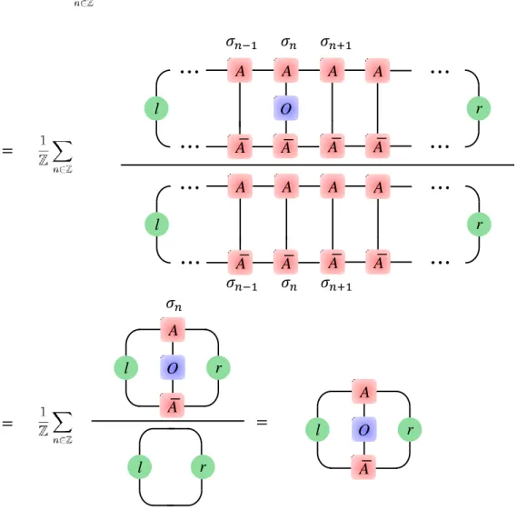
Suppose we want to compute the expectation value ⟨O⟩ with operator

⟨O⟩ =∑

n∈Z

1

ZOn, (3.19)

whereZ represents the number of sites. Since translation invariance, so ⟨O⟩ can be represented as in Fig. 3.4.

A

A O

l r

𝜎_𝑛

A

A O A

A A

A A

l

⋯

⋯

⋯

⋯

A

r 𝜎_𝑛

𝜎_𝑛−1 𝜎_𝑛+1

A

A O

l r

=

= =

l r

A

A A

A A

A A

l

⋯

⋯

⋯

⋯

A

r

𝜎_𝑛

𝜎_𝑛−1 𝜎_𝑛+1

Figure 3.4: Expectation value represented as a tensor network diagram.

3.5 Gauge Degrees of Freedom, Canonical Form and Symmetric gauge

There is no unique way to write down a uMPS to represent a given quantum state on a 1D infinite lattice. For a given uMPS |ψ(A)⟩, we can use a local gauge transformation A^s → XA^sX⁻¹, with invertible X ∈ ^CD×D to represent the same quantum state. Namely,|ψ(A)⟩ = |ψ(XAX⁻¹)⟩, since

⋯

|𝜓(𝑋𝐴𝑋⁻¹)

A A A

⋯

⋯

=

⋯

A 𝑋⁻¹

X X A 𝑋⁻¹ X A 𝑋⁻¹

I I I I

=

= |𝜓(𝐴) . ^(3.20)

We introduce Γ, Λ notation to represent uMPS. For a given uMPS|ψ(A)⟩ , we can use SVD to decompose the uMPS as in Fig. 3.5, denoting the diagonal term as Λ and the other term as Γ. In other words, we can use (Λ,Γ) to represent uMPS.

⋯

Г Г

Λ Λ Λ

A

→

(a)

A

A A

⋯ ⋯

→

→ ⋯

⋯

(b)

Figure 3.5: (a) Use SVD to decompose tensor A. (b) (Λ,Γ) notation for uMPS.

Furthermore, we say (Λ,Γ) is canonical if

doi:10.6342/NTU201802766 Г

Г

=

Г

Г

=

,

Λ

Λ

Λ

Λ

.

(3.21)

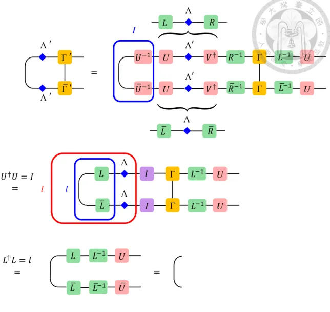
An arbitrary uMPS (Λ,Γ) is not generically canonical, but it can be changed to the canonical form using a gauge transformation [15]. We will show the step by step process to change an arbitrary uMPS (Λ,Γ) to the canonical form (Λ^′,Γ^′). First, we need to find the eigentensors l and r by solving the following eigenvalue equations,

r Г

Г

=

Г

Г

=

,

l l r

Λ

Λ Λ

Λ

.

Notice that tensor l and r are Hermitian after simple resized. Then we find the matrices L and R such that L^†L = l and RR^† = r, so we can choose L = l¹² and R = r¹². Finally, we insert these matrices and do SVD as following step:

Λ

Г

Λ

⋯ ⋯

↓ ↓

↓

↓

𝐼 𝐼

𝐼 𝐼

𝐿⁻¹ 𝐿 𝑅 Г 𝐿⁻¹ 𝐿 𝑅⁻¹ 𝑅

⋯ ⋯

↓

↓

U 𝑉^†

Λ^′

U 𝑉^†

Λ^′

𝐿⁻¹ Г 𝐿⁻¹ 𝑅

⋯

⋯

′

U 𝑉^†

Λ^′ Г^′

Λ^′

Г^′

Λ^′

⋯ ⋯

=

=

=

𝑅⁻¹

𝑅⁻¹

. ^(3.23)

Г ^′

= Λ ^′

Λ ^′ Г ^′

l

Г Λ

U

Г Λ

U 𝐼

𝐼 𝐿

𝐿

𝐿⁻¹

𝐿⁻¹ l

𝐿 𝑅

Λ

𝑈⁻¹

𝑈⁻¹

𝑉^† Г Λ^′

U

𝑉^† Г Λ^′

U U

U

𝐿 𝑅

Λ

𝑅⁻¹ 𝐿⁻¹

𝑅⁻¹ 𝐿⁻¹

I

𝑈^†𝑈 = 𝐼

𝐿^†𝐿 = 𝑙

=

𝐿⁻¹ U

𝐿⁻¹ U 𝐿

𝐿

= =

Figure 3.6: Check the property of the left canonical form.

Then we get the canonical form (Λ^′,Γ^′) and we can easily check the left-canonical form property (as in Fig. 3.6) and also for the right canonical form property. Now we can construct a unit tensor again by using canonical (Λ,Γ) as

A Г

Λ

= A Г

Λ

=

(a) left canonical form (b) right canonical form

(3.24)

Another special gauge we shall introduce here is symmetric gauge, which can be constructed by canonical (Λ,Γ) as

A Г

Λ¹²

=

Λ¹² .

(3.25)

doi:10.6342/NTU201802766 We can observe that the left and right eigenvectors of this kind of transfer matrix

are Λ, since

Λ

,

Г

Г

= Λ¹² Λ¹²

Λ¹² Λ¹² Λ

Г

Г

= Λ¹²

Λ¹² Λ

𝐼

Λ

Λ Г

Г

= Λ¹²

Λ¹²

Λ¹² Λ¹²

Λ

Г

Г

= Λ¹²

Λ¹²

Λ

𝐼

Λ

.

(3.26)

(3.27)

Finally, we will introduce the mixed canonical form for uMPS. For a given canon- ical (Λ,Γ), we can construct mixed-canonical form:

⋯

𝐴_𝑅 𝐴_𝐿 𝐴_𝐿 𝐴_𝐿

⋯

⋯

𝐴_𝑅

𝐴_𝐿 𝐴_𝐿 𝐴_𝐶

⋯

=

(3.28)

Here, AL is left-canonical tensor and AR is right-canonical tensor that can be con- structed as above, and we define new tensors A_C and C which can be constructed by

𝐴_𝐶 Г

Λ

=

Λ

,

C =

Λ

.

(3.29)

The tensors A_L, A_R, A_C ,C in mixed-canonical form need to satisfy the condition

A^s_LC = A_C = CA^s_R, (3.30)

or diagrammatically,

𝐴_𝐿 C = 𝐴_𝐶 = C 𝐴_𝐿

. ^(3.31)

3.6 Geometric Series for Transfer Matrix

At Chapter 4 and 5, we will introduce two algorithms (time-dependent varia- tional principle and variational optimization method for uMPS) and both of them are needed to simulate the geometric series of the transfer matrix. We know that for a given uMPS|ψ(A)⟩, which the corresponding unit tensor A has been normalized, we can define the transfer matrix E =∑

sA^s⊗ ¯A^s and its leading eigenvalue is one.

If we want to calculate the geometric series of E, we can use the formula:

∑∞ i=0

Eⁱ = I + E + E²+ E³ +· · · = (I − E)⁻¹. (3.32) First, we diagonalize the transfer matrix

D = P⁻¹EP =









1 0 0 0

0 λ₁ 0 0 0 0 λ₂ 0 0 0 0 . ..









, (3.33)

where 1 > λ1 > λ2 >· · · are the eigenvalues of the transfer matrix E. Then,

P⁻¹(I− E) P = I − P⁻¹EP =









0 0 0 0

0 1− λ1 0 0 0 0 1− λ2 0

0 0 0 . ..









=









0 0 0 0

0 λ˜₁ 0 0 0 0 λ˜₂ 0 0 0 0 . ..







 ,

(3.34)

where ˜λ_i = 1− λ, for all i = 1, 2, 3 · · ·. Define ˜D = P⁻¹(I− E) P = I − P⁻¹EP , then I−E = P ˜DP⁻¹. We can clearly see that the determinant of matrix I−E is 0, which implies the matrix I− E is not invertible. So we define the pseudo-inverse¹

(I− E)^P = P









0 0 0 0

0 λ˜1

−1 0 0

0 0 λ˜₂⁻¹ 0

0 0 0 . ..









P⁻¹. (3.35)

1We can see the idea of pseudo-inverse from Ref. [6].

doi:10.6342/NTU201802766 If {⟨˜li|} and {|˜ri⟩} are the set of eigenvectors of matrix I − E, and ⟨l| and |r⟩ are

the leading eigenvectors of transfer matrix E. Then,

(I− E) = ˜λ0|˜r0⟩⟨˜l0| + ˜λ1|˜r1⟩⟨˜l1| + ˜λ2|˜r2⟩⟨˜l2| + · · · + ˜λn−1|˜rn−1⟩⟨˜ln−1|, (3.36) where n = D× D and λ0 = 0. We can rewrite the pseudo-inverse as

(I− E)^P = ˜λ⁻¹₁ |˜r1⟩⟨˜l1| + ˜λ₂|˜r2⟩⟨˜l2 +· · · + ˜λ⁻¹_n−1|˜rn−1⟩⟨˜ln−1| (3.37) and Eq. (3.36) implies that

I− (E − |r⟩⟨l|) = |r⟩⟨l| + ˜λ1|˜r1⟩⟨˜l1| + ˜λ2|˜r2⟩⟨˜l2| + · · · + ˜λn−1|˜rn−1⟩⟨˜ln−1| (3.38) If we inverse the Eq. (3.38), then we get

[I− (E − |r⟩⟨l|)]⁻¹

=|r⟩⟨l| + ˜λ⁻¹1 |˜r1⟩⟨˜l1| + ˜λ₂⁻¹|˜r2⟩⟨˜l2| + · · · + ˜λ⁻¹n−1|.˜rn−1⟩⟨˜ln−1|. (3.39) Compare the Eq. (3.37) and Eq. (3.39), we can rewrite the pseudo-inverse of I− E as

(I− E)^P = [I− (E − |r⟩⟨l|)]⁻¹− |r⟩⟨l|. (3.40) In many cases, we need to operate a given left tensor or right tensor with (I− E)^P. For instance, given a tensor hl, we want to calculate tensor K:

𝐼 − 𝐸 ^𝑃 =

ℎ_𝑙 K (3.41)

and we can denote it as

⟨K| = ⟨hl|(I − E)^P. (3.42)

According to Eq. (3.40), we have:

⟨K| = ⟨hl| [I − (E − |r⟩⟨l|)]⁻¹− ⟨hl|r⟩⟨l| (3.43) Then,

[⟨K| + ⟨hl|r⟩⟨l|] [I − (E − |r⟩⟨l|)] = ⟨hl|

⇒⟨K| [I − (E − |r⟩⟨l|)] + ⟨hl|r⟩⟨l| − ⟨hl|r⟩⟨l|E + ⟨hl|r⟩⟨l|r⟩⟨l| = ⟨hl| (3.44) Since⟨l|E = ⟨l| and ⟨l|r⟩ = 1, the Eq. (3.44) becomes

⟨K| [I − (E − |r⟩⟨l|)] + ⟨hl|r⟩⟨l| − ⟨hl|r⟩⟨l| + ⟨hl|r⟩⟨l| = ⟨hl|, (3.45)

which implies

⟨K| [I − (E − |r⟩⟨l|)] = ⟨hl| − ⟨hl|r⟩⟨l|. (3.46) Tensor h_lis given, so we can solve the linear equation to obtain the tensor K. Rather than invert the matrix I−E+|r⟩⟨l| directly, we can use biconjugate gradient stabilized method (BiCGSTAB) [16], which is a Krylov subspace method, to solve the linear equation. Its computational complexity is just O(D³). And we can follow the same procedure to contract right tensor with (I− E)^P.

3.7 Matrix Product Operator

In many cases, we can write the Hamiltonian in matrix product operator (MPO) form; for instance, the Hamiltonian of Heisenberg model is:

H = J 2

∑

n

(S_n⁺S_n+1⁻ + S_n⁻S_n+1⁺ )

+ J_zS_n^z (3.47) If we define an operator

   

































I S J S J S J S S S I O

z z z

i

ˆ ˆ 2 ˆ

ˆ / 2 / 0

0 0 0

ˆ 0

0 0 0

ˆ 0

0 0 0

ˆ 0

0 0 0

ˆ 0

ˆ^[] O ^(3.48)

Then we can make the Heisenberg model as a product of these operators H =∏

n

O^[i] (3.49)

or graphically as:

O O O O

⋯ ⋯ ^(3.50)

For the Thirring model [Eqs. (2.12) and (2.13)] (with Starget = 0), we can write

doi:10.6342/NTU201802766 down the MPO as

O^[n] =















I 0 0 0 0 0

S⁻ 0 0 0 0 0

S⁺ 0 0 0 0 0

S^z 0 0 I 0 0

S^z 0 0 0 0 0

β_nS^z + γI −_2a¹S⁺ −_2a¹S⁻ 2λS^{z ∆}_aS^z I















, (3.51)

where

β_n = ∆

a + (−1)ⁿm γ = λ

4 + ∆ 4a.

Since this MPO acts on local pairs of sites can be represented as a tensor network diagram

⋯ 𝑂₁ 𝑂₂ 𝑂₁ 𝑂₂ ⋯

.

(3.52)

This kind of MPO form is not invariant under single-site translation, so we merge two MPO to one by:

𝑂₁ 𝑂₂ = 𝑂

2 2 4

(3.53)

In this thesis, we choose physical bond dimension d = 4 for uMPS.

We have already found the MPO form for the Thirring model, so we can use tensor network method to find the ground state of the Thirring model and do real- time evolution for it. We are going to introduce the time-dependent variational principle (TDVP) algorithm and variational uMPS algorithm (VUMPS) at next two chapter.

Chapter 4

Variational Optimization Method for uniform Matrix Product State

The variational optimization method for uniform matrix product state (VUMPS) [5] algorithm is a variational tensor network algorithm for determining the ground state of many-body systems on 1D lattices.

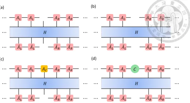
4.1 Effective Hamiltonian

In most many-body systems, it is impossible to directly determine the ground state, even for simple nearest neighbour Hamiltonians. Instead, we will introduce an effective Hamiltonian. For a given mixed canonical uMPS (A_L, A_R, C), we can define the one-site effective Hamiltonian and zero-site effective Hamiltonian as in Fig. 4.1. It is much easier to find the ground state of the effective Hamiltonian.

If we use MPO to represent the effective Hamiltonian, it can be represented as:

𝐴_𝐿 𝐴_𝐿 𝐴_𝑅 𝐴_𝑅

𝐴 _𝐿 𝐴 _𝐿 𝐴 _𝑅 𝐴 _𝑅

⋯

⋯

⋯

⋯

⋯

⋯

𝑂 𝑂 𝑂 𝑂 𝑂

(a) single–site effective hamiltonian:

𝐴_𝐿 𝐴_𝐿 𝐴_𝑅 𝐴_𝑅

𝐴 _𝐿 𝐴 _𝐿 𝐴 _𝑅 𝐴 _𝑅

⋯

⋯

⋯

⋯

⋯

⋯

𝑂 𝑂 𝑂 𝑂

(b) zero–site effective hamiltonian:

(4.1)

(4.2)

doi:10.6342/NTU201802766

𝐻

𝐴_𝐿 𝐴_𝐿 𝐴_𝑅 𝐴_𝑅

𝐴 _𝐿 𝐴 _𝐿 𝐴 _𝑅 𝐴 _𝑅

⋯

⋯

⋯

⋯

⋯

⋯

𝐻

𝐴_𝐿 𝐴_𝐿 𝐴_𝑅 𝐴_𝑅

𝐴 _𝐿 𝐴 _𝐿 𝐴 _𝑅 𝐴 _𝑅

⋯

⋯

⋯

⋯

⋯

⋯

𝐻

𝐴_𝐿 𝐴_𝐿 𝐴_𝑅 𝐴_𝑅

𝐴 _𝐿 𝐴 _𝐿 𝐴 _𝑅 𝐴 _𝑅

⋯

⋯

⋯

⋯

⋯

⋯

𝐴_𝐶

𝐻

𝐴_𝐿 𝐴_𝐿 𝐴_𝑅 𝐴_𝑅

𝐴 _𝐿 𝐴 _𝐿 𝐴 _𝑅 𝐴 _𝑅

⋯

⋯

⋯

⋯

⋯

⋯

𝐶

(a) (b)

(c) (d)

Figure 4.1: (a) One-site effective Hamiltonian, (b) zero-site effective Hamiltonian (c) acting with tensor A_C on one-site effective Hamiltonian (d) acting with tensor C on zero-site effective Hamiltonian.

In practice, we need to find a block tensor L such that

𝐿 =

𝐴_𝐿 𝐴_𝐿

𝐴 _𝐿 𝐴 _𝐿

⋯

⋯

⋯

𝑂 𝑂 𝑅 =

𝐴_𝑅 𝐴_𝑅

𝐴 _𝑅 𝐴 _𝑅

⋯

⋯

⋯

𝑂 𝑂

, .

(4.3)

For instance, the MPO of the Thirring model with penalty term can be represented by the following form

𝛼 𝛽 1 2 3 4 5 6 1

2 3 4 5 6 𝛼 𝑂 𝛽

= . ^(4.4)

And we can see that tensor L will satisfy

𝐿 𝐿 =

𝐴_𝐿

𝐴 _𝐿 𝛼 𝑂 𝛽

𝛽 . (4.5)

We can represent the tensor L as a set of tensors:

𝐿 = 𝐿₁ 𝐿₂ 𝐿₃ 𝐿₄ 𝐿₅ 𝐿₆

, , , , ,

𝛽 . ^(4.6)

Then, construct the tensor L order by order. For β = 6,

𝐿₆ 𝐿₆

𝐴_𝐿

𝐴 _𝐿

= 𝐼 𝐿₆ = . ^(4.7)

For β = 2, 3, 5,

𝐿_𝑖 𝐿₆

𝐴_𝐿

𝐴 _𝐿 𝑌_𝑖

= =

𝐴_𝐿

𝐴 _𝐿

𝑌_𝑖 , 𝑖 = 2,3,5 . _(4.8)

For β = 4,

𝐿₄ 𝐿₁

𝐴_𝐿

𝐴 _𝐿 𝑌₄

= + 𝐿₄

𝐴_𝐿

𝐴 _𝐿

𝐼 . (4.9)

Or we can denote it as

L₄(n + 1) = T_L(L₄(n)) + C₁, (4.10)