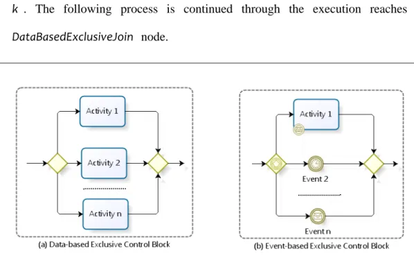
運用一具Hierarchy 特性的Timed CPNets 技術來分析BPMN 工作流程

(1)

國

立

交

通

大

學

資訊科學與工程研究所

博

士

論

文

運用一具 Hierarchy 特性的 Timed CPNets 技

術來分析 BPMN 工作流程

Applying Timed CPNets with Hierarchy to Analyze a

Workflow in BPMN

研究生：王靜慧

指導教授：王豐堅教授

中華民國九十八年七月

(2)

運用一具 Hierarchy 特性的 Timed CPNets 技術來分析

BPMN 工作流程

Applying Timed CPNets with Hierarchy to Analyze a

Workflow in BPMN

研究生：王靜慧 Student：Ching-Huey Wang

指導教授：王豐堅 Advisor：Feng-Jian Wang

國立交通大學

資訊科學與工程研究所

博士論文

A Thesis

Submitted to Institute of Computer Science and Engineering College of Computer Science

National Chiao Tung University in partial Fulfillment of the Requirements

for the Degree of Doctor

in Computer Science

July 2009

Hsinchu, Taiwan, Republic of China

(3)

運用一具 Hierarchy 特性的 Time CPNets 技術來分析

BPMN 工作流程

學生：王靜慧指導教授：王豐堅博士

國立交通大學資訊工程與科學研究所博士班

摘要

相對於 BPMN 而言，現存的商業流程之研究或商業軟體大多只提供或使用其中的部分。BPMN 主要的組成元素包括:控制流程、訊息流程、資料流程以及角色分配。它也提供多實體 activity、事件觸發 activity 及進階控制機制。雖然這些元素讓 BPMN 具更大的流程表達能力，但也增加了設計階段其所表達之流程的分析困難度。本論文提出一個正規流程模型來協助根據 BPMN 四種組成元素所描述的商業流程。同時，也提供一具階層特質之時間顏色派翠網模型。並建立一套流程與此網的轉換規則，以便將上述 BPMN 商業流程轉換成相對之時間顏色派翠網，來運用既有之分析方法做靜態分析—如 deadlock 檢查。在本論文中，我們更進一步探討 well-formed 和 unstructured 相當普遍的流程之分析。此外，我們將以一個實際的例子做示範，利用時間顏色派翠網 deadlock 分析方法，再根據其結果推斷可能會影響流程執行的異常 artifact 之使用。最後，我們也將比較刻下技術與我們之研究成果。關鍵字: 商業流程模型符號，工作流程，商業流程，分析，控制流程，資料流程，訊息流程、顏色派翠網、時間顏色派翠網、階層式派翠網

(4)

Applying Timed CPNets with Hierarchy to Analyze a

Workflow in BPMN

Student：Ching-Huey Wang Advisor：Dr. Feng-Jian Wang

Institute of Computer Science and Engineering

National Chiao Tung University

Abstract

Although many business process models have been proposed, most of them do not apply all the following arguments: control, message and data flows and role

assignments, defined completely in BPMN. Besides, they do not provide the

multi-instance activity, event-triggered activity or the control node with complex mechanisms as in BPMN. On the other hand, these features allow a process to be defined with richer semantics but increase the difficulty of correcting an error or inaccurate process in workflow design.

This thesis proposes a formal process model to help describing a BPMN-based process. To simplify the analysis, we also provided Hierarchical Timed Coloured Petri Nets (H PNets), which is extended from Time Coloured Petri Nets with _CT

hierarchy and allows some analysis with existing techniques. Once a workflow based on our BPMN model is specified, a series of mapping rules can be used to transform the workflow into a H PNets for analysis. An example is applied to demonstrate the T_C

transformation and the corresponding deadlock detection. Furthermore, the artifact usage anomaly detection mechanisms within either a well-formed or unstructured

(5)

process are discussed. Finally, a comparison among related works and ours and the future works are presented.

Keyword: BPMN, workflow, business process, analysis, control flow, data flow, message flow, CPNets, Time CPNets and hierarchical PNets.

(6)

誌謝

本篇論文的完成，首先要萬分感謝指導教授王豐堅博士，王教授在我求學期間持續不斷的指導與鼓勵，讓我不僅在論文研究方面學習到相當寶貴的經驗，在做人處事方面也獲益良多。如今學生若有些微的成就，王教授的指導實在功不可沒。其次要感謝吳毅成教授，陳耀宗教授，朱治平教授，黃冠寰教授，焦惠津教授，梅興教授，與楊鎮華教授，在百忙之中首肯擔任我博士論文的口試委員，並且提供了許多寶貴的意見，補足我論文裡不足的部分。其中吳、陳兩位教授亦是我的論文計畫書口試委員，在論文報告的方式上也給了我相當多的指導。此外，對於一起研究討論與互相鼓勵的實驗室學長與學弟們，包括楊基載、黃國展、王建偉、許嘉麟、許懷中、黃培書等等，在此一併加以感謝。最後，我要與我的家人、同學、朋友共同分享完成論文的喜悅，由於有您們的支持與關懷，陪伴我走過這漫長的求學過程。僅將此論文獻給我最敬愛的父母親與支持我的親友們。

(7)

List of Figures and Tables

FIGURE 2.1 AN EXAMPLE OF A PNET. ... 4

FIGURE 2.2 AN EXAMPLE OF CPNET. ... 13

FIGURE 2.3 THE RESULT NET OF FIRING STEP Y₁. ... 18

FIGURE 2.4 INTRODUCING TIME CONSTRAINTS INTO THE CPNET SHOWN IN FIGURE 2.1. ... 21

FIGURE 2.5 THE RESULT NET OF FIRING STEP Y₁. ... 24

FIGURE 2.6 AN EXAMPLE OF H_CTPNET. ... 26

FIGURE 3.1 THE CORE MODELING ELEMENTS IN BPMN. ... 31

FIGURE 3.2 E‐MAIL VOTING PROCESS ... 32

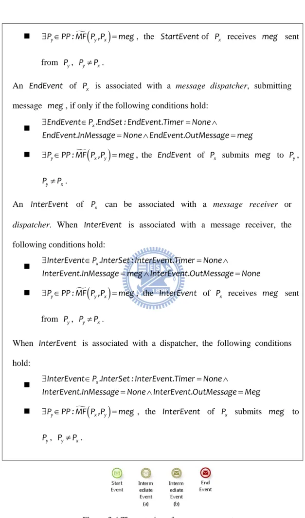
FIGURE 3.3 THE NOTATIONS FOR NONE EVENTS. ... 38 FIGURE 3.4 THE NOTATIONS FOR MESSAGE EVENTS. ... 39 FIGURE 3.5 THE NOTATIONS FOR THE TIMING EVENTS. ... 40 FIGURE 3.6 THE CASES OF SUPPLEMENT ARCS. ... 45 FIGURE 3.7 AN ACTIVITY WITH A MESSAGE DISPATCHER. ... 45 FIGURE 3.8 NOTATIONS FOR LOOP ACTIVITIES. ... 50 FIGURE 3.9 SAMPLES OF EXCLUSIVE CONTROL BLOCK. ... 54 FIGURE 3.10 A SAMPLE OF INCLUSIVE CONTROL BLOCK. ... 55 FIGURE 3.11 A SAMPLE OF PARALLEL CONTROL BLOCK. ... 55 FIGURE 3.12 SAMPLES OF LOOP CONTROL BLOCK. ... 57 FIGURE 3.13 THE SAMPLES OF COMPLEX BLOCKS. ... 58 FIGURE 3.14 THE CONTROL FLOW OF THE BUSINESS PROCESS FOR RESOLVING ISSUES. ... 60

FIGURE 3.15 THE EXPANSION OF COLLECT VOTE SUB‐PROCESS. ... 61

FIGURE 3.16 THE STATE TRANSITION DIAGRAM OF AN ARTIFACT. ... 63

FIGURE 3.17 THREE CASES OF INCOMING DATA FLOWS. ... 66

FIGURE 3.18 THE FOUR CASES OF INTERMEDIATE DATA FLOWS. ... 67

FIGURE 3.19 THE CONTROL AND DATA FLOWS OF BPVOTE. ... 68

FIGURE 3.20 THE EXPANSION OF “COLLECT VOTES” SUB‐PROCESS. ... 70

FIGURE 4.1 AN EXAMPLE OF OVERLAPPED STRUCTURE. ... 75

(10)

FIGURE 5.1 TWO DIFFERENT PRESENTATIONS OF THE STATE TRANSITIONS OF A PROCESS INSTANCE. ... 77

FIGURE 5.2 THE MAPPING OF THE ELEMENTS ADDRESSED IN [29]. ... 81

FIGURE 5.3 COMBINING THE EXPANSION OF A SUB‐PROCESS AND PARENT NET. ... 81

FIGURE 5.4 THE MAPPING OF THE CONTROL NODES ADDRESSED IN [29]. ... 82

FIGURE 5.5 TWO DIFFERENT H_CTPNETS MODULES OF A TASK WITH LOOP STRUCTURE. ... 85

FIGURE 5.6 FOUR DIFFERENT HT_CPNETS MODULES OF A TASK WITH MULTI‐INSTANCE LOOP STRUCTURE. ... 87

FIGURE 5.7 THE H_CTPNETS MODULE OF INTERMEDIATE EVENT. ... 87

FIGURE 5.8 TWO DIFFERENT PRESENTATIONS OF MESSAGE START EVENT. ... 89

FIGURE 5.9 TWO DIFFERENT PRESENTATIONS OF INTERMEDIATE MESSAGE DISPATCHER. ... 90

FIGURE 5.10 TWO DIFFERENT PRESENTATIONS OF A TASK INVOLVING A TIMING EVENT. ... 90

FIGURE 5.11 TWO DIFFERENT PRESENTATIONS OF A TASK INVOLVING A MESSAGE RECEIVER. ... 91

FIGURE 5.12 TWO DIFFERENT PRESENTATIONS OF A SUB‐PROCESS INVOLVING A MESSAGE RECEIVER. ... 91

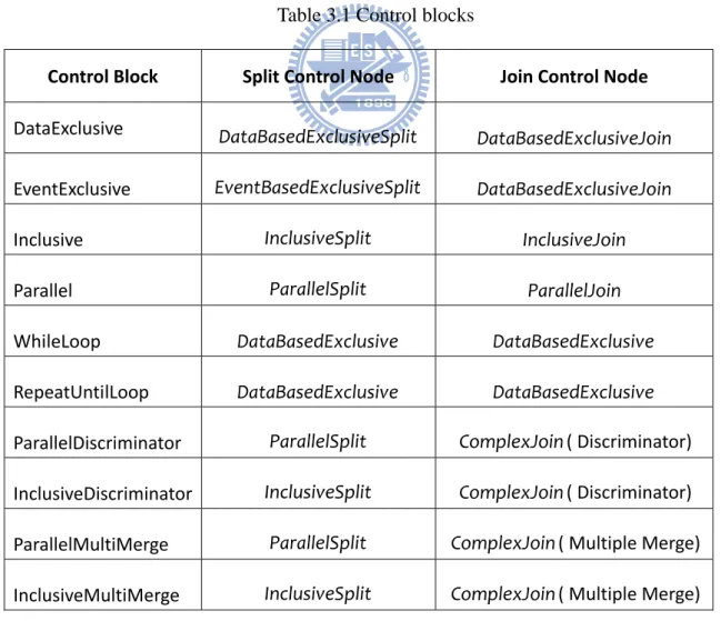
FIGURE 5.13 TWO DIFFERENT PRESENTATIONS OF A TASK INVOLVING A MESSAGE DISPATCHER. ... 92 FIGURE 5.14 DIFFERENT PRESENTATIONS OF A COMPLEX CONTROL NODE IMPLEMENTED WITH DIFFERENT MECHANISMS. . 93 FIGURE 5.15 TWO DIFFERENT PRESENTATIONS OF A MESSAGE FLOW BETWEEN TWO TASKS. ... 94 FIGURE 5.16 TWO DIFFERENT PRESENTATIONS OF A MESSAGE FLOW BETWEEN A TASK AND A START EVENT. ... 95 FIGURE 5.17 TWO DIFFERENT PRESENTATIONS OF A MESSAGE FLOW BETWEEN A TASK AND AN INTERMEDIATE EVENT. ... 96 FIGURE 5.18 A MESSAGE FLOW BETWEEN AN INTERMEDIATE EVENT AND A TASK. ... 96 FIGURE 5.19 A MESSAGE FLOW BETWEEN INTERMEDIATE AND START EVENTS. ... 97 FIGURE 5.20 A MESSAGE FLOW BETWEEN TWO INTERMEDIATE EVENTS. ... 97 FIGURE 5.21 TWO DIFFERENT PRESENTATIONS OF A MESSAGE FLOW BETWEEN AN END EVENT AND A TASK. ... 98 FIGURE 5.22 TWO DIFFERENT PRESENTATIONS OF A MESSAGE FLOW BETWEEN AN END EVENT AND A START EVENT. ... 99 FIGURE 5.23 TWO DIFFERENT PRESENTATIONS OF THE STATE TRANSITION OF AN ARTIFACT. ... 101 FIGURE 5.24 A HT_CPNETS MODULE OF INCOMING DATA FLOWS. ... 101 FIGURE 5.25 A HT_CPNETS MODULE OF INTERMEDIATE DATA FLOWS... 103 FIGURE 5.26 A HT_CPNETS MODULE OF INTERMEDIATE DATA FLOWS. ... 105 FIGURE 6.1 TWO PRESENTATIONS OF THE EMAIL VOTING EXAMPLE. ... 111 TABLE 3.1 CONTROL BLOCKS ... 58

TABLE 3.2 ARTIFACTS IN THE E‐MAIL VOTING PROCESS ... 68

(11)

TABLE 5.1 THE NOTATIONS AVAILABLE IN PROCESS MODEL [29]. ... 83

TABLE 6.1 THE FIRING SEQUENCE OF PROCESS BP_vote ... 110

TABLE 7.1 THE MAPPINGS OF THE ELEMENTS IN MESSAGE FLOW ADDRESSED. ... 112

TABLE 7.2 THE MAPPINGS OF THE ELEMENTS OF CONTROL FLOW ADDRESSED. ... 113

TABLE 7.3 THE MAPPING OF THE ELEMENTS OF DATA FLOW ADDRESSED. ... 114

(12)

Chapter 1. Introduction

Workflow can be viewed as a set of interrelated tasks that are systematized to achieve certain business goals by completing the tasks in a particular order under automatic control [1]. The Business Process Modeling Notation (BPMN) [2] is a standard for capturing workflow in the early phases of system development. Existing researches focus on 1) parts of the concepts included in BPMN only, e.g., control flow analysis[3][48] or 2) how to transform from control and message flow in BPMN into BPEL code [4][5][6].

A BPMN-based workflow is described with four entities: 1) role: describing the performers of task instantiated, 2): control flow: defining what, when and how tasks a workflow performs, 3) data flow: specifying what information entities are produced/manipulated/passed in corresponding activities and 4) message flow: representing the interaction between processes through messages. An analysis based on the correlations among these four entities can help check or maintain consistency between execution order and data transition [7][8][9][10], as well as prevents exceptions due to contradiction between data flow, control and message interaction.

There are five additional features introduced in BPMN, but not included in traditional process modeling languages. These features allow defining: 1) an interaction between participants, 2) a multi-instance (loop) activity 3) an event-triggered (supplement) process, 4) a join node designed by one of the three advanced join mechanisms, discriminator, multiple merge and N out of M join, and 5) a data flow described with explicit channel. In addition, time event-triggered behaviors can be described in a BPMN-based workflow, i.e., time constrains are embedded. These features allow defining a process with richer semantics, but increase

(13)

the difficulty of identifying the problems such as inaccuracy in a process specification at design time.

Here, we provide an easier way to extract knowledge from the four entities of a workflow. Based on our previous work [11], a method for describing a BPMN-based process is proposed. Then, we propose a model, Hierarchical Timed Coloured Petri Nets (H PNets), extended from Timed Coloured Petri Nets (TCPNets) with hierarchy T_C

[13][14] for analysis. There are a series of mapping rules defined to transform a BPMN-based process into H PNets, in which a set of analysis techniques works T_C [14].

With our methodology, the artifact usage anomalies in our previous work are refined. An analysis method of control, data, and message flow is derived. An example is used to indicate our contribution of process development and anomaly detections. Finally, a comparison among ours and related works is presented.

The remainder of this paper is organized as follows. Chapter 2 introduces the Petri Nets and its extensions, Coloured Petri Nets (CPNets), and TCPNets. It also compares existing flow specification model and BPMN. Besides, H PNets is T_C

proposed for the problems identified. Chapter 3 presents our business process model, including the control flow, data flow and message flow. In Chapter 4, we present a set of rules transforming a process in BPMN into H PNets. In Chapter 5, the T_C

well-behaved unstructured processes are identified and formulated. In Chapter 6, we present a case to demonstrate our methodologies including development and analysis. A comparison between our approach and related works on BPMN is given in Chapter 7. Finally, a conclusion and some recommendations of future works are given in Chapter 8.

(14)

Chapter 2. Petri Nets – PNets

PNets, Petri Nets, is a formal model with graphical representations. The original PNets was developed by Petri [27], and various extensions have been developed with their own constructs. Some of these extensions are associated with easier modeling mechanism and keep the same expressiveness as classical PNets [28] and some provide more expressional power [22][23]. PNets has been applied to many areas, including workflow applications [29][30][31]. In this chapter, we discuss the problems rising when applying PNets or its extensions, Coloured Petri Nets and Time

Petri Nets, to analyze business processes represented with BPMN. Before the

discussion, definitions of PNets and the two extensions are given. 2.1. Definition of Classical Petri Nets

A PNet, defined in Definition 2.1, is a directed graph with two kinds of nodes, named place and transition. In general, a place is presented with a circle while a transition is presented with a rectangle. There are no arcs connecting two places or two transitions. An example of PNet is shown in Figure 2.1 where there are three places, two transitions and one token.

Definition 2.1 (Classical Petri Nets – PNets) A Petri net is a 4-tuple PNet=

(

P,T ,F ,m₀

)

where 1. P is a finite set of places,

2. T is a finite set of transitions such that P∩ =T φ,

(15)

(

)

(

)

φ

∩ × = ∩ × =

F P P F T T ,

4. m is the initial marking function, ₀ m : P0 → where = , ,...

{

1 2

}

.

Figure 2.1 An example of a PNet.

Definition 2.2 (Marking)

1. A marking M of a set of places P is a mapping m : P→ where

{

0 1 2, , ,...

}

= .

2. A marking M of a Petri net PNet=

(

P,T ,F ,m0

)

is a marking of P . Initial

marking M of PNet is generated by function 0 m . 0

In Definition 2.2, function m is defined from a place to a nonnegative integer

which means the number of tokens on the place. A PNet is also equipped with an

initial marking M , i.e., an initial state of the PNet is associated with one or more ₀

token in some place(s). All the states of this net succeed to M , generated by function ₀

0

m . Marking M of an example PNet shown in Figure 2.1 can be expressed as an 0

array based on the order

(

p ,p ,p₀ ₁ ₂

)

with nonnegative integers

(

1 0 0, ,

)

. Definition 2.3 (Input/Output Set)

Let PNet=

(

P,T ,F ,m₀

)

be a Petri net, for an element x P∈ ∪T

(16)

1. _{its input set} •x is defined as •x= ∈ ∪

{

y P T | y,x

( )

∈F and

}

2. _{its output set} x is defined as • x•= ∈ ∪

{

y P T | x,y

( )

∈F .

}

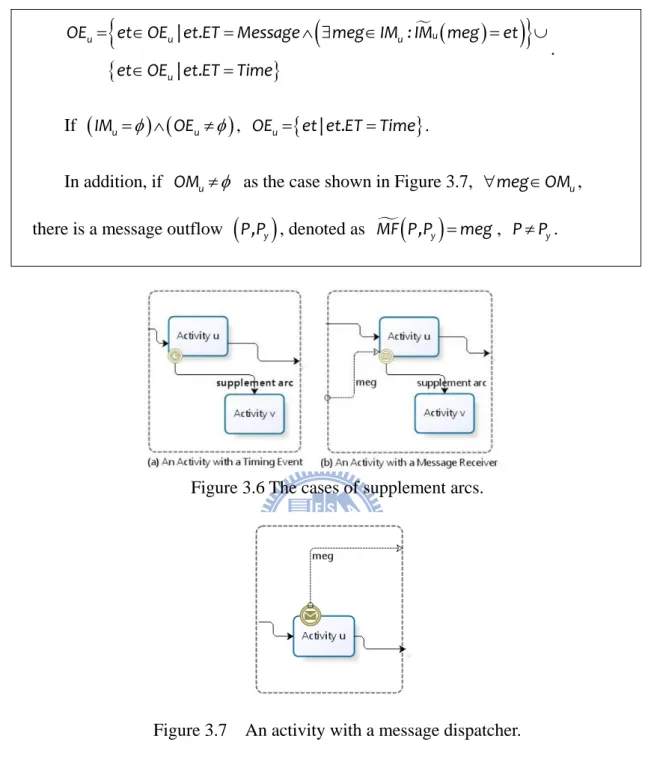
Definition 2.3 defines the notations about the input and output sets of a node (place or transition) in a PNet. Note that both sets of a place contain transitions only and both sets of a transition contain places only.

Definition 2.4 (Fire a Transition Enabled)

A transition _{t is able to be fired (named as enabled) if} ∀ ∈p •t , m p

( )

≥1. Firing t transforms marking M into marking M' and the transformation can be

defined from place _{p by function m and m' as}

( )

1 1 − ∈ − ⎧ ⎪ =_⎨ + ∈ − ⎪ ⎩ • • • • m p if p t t , m' p m p if p t t, m(p) otherwise.

When t is enabled in M , t may fire to change marking M to another

marking _{M' . The new marking M' is obtained by removing one token from each of} its input places •t and by putting one token to each of its output places •

t . M' is

also called directly reachable from M with firing of t , denoted as M t M'

[

.

A finite occurrence (of firing) sequence is M t1⎣⎡ 1 M t2⎡⎣ 2 M ...M3 n−1

[

tn−1 M n

where M t_i[_i M_i₊₁ , 1≤ ≤ . Marking i n M is called start marking of the occurrence 1

sequence, while M is called the end marking. The non-negative integer _n n−1_is called the number of steps in the occurrence sequence.

(17)

Definition 2.5 (Reachable)

A marking M is reachable from a marking _n M iff there is a finite ₁

occurrence sequence whose start/end markings are M /₁ M correspondingly _n

[

1⎡⎣ 1 2⎡⎣ 2 3 n−1 n−1 n

M t M t M ...M t M

n

M is reachable from M₁ in n−1_{steps. The set of markings which are reachable} from M is denoted by ₁

[

M1 .

2.1.1. Advantages of PNets Adoption

Many researches [29][30][31][32][33][34][39]proposed workflow modeling and analysis paradigms based on PNets, e.g., control/data flow modeling [31][32][33], workflow pattern composition [35][36][37][46], and automatic control of workflow process [38]. Aalst and ter Hofstede [39] proposed a WorkFlow net (WF-net) based on PNets to model a workflow: Transitions represent activities, places represent conditions, tokens represent cases (process instances), and directed arcs connecting transitions and places. Concluding by Aalst [40], the advantages of adopting PNets to analyze process are : (1) presenting a process with formal expression keeps the verifiability of PNets, (2) utilizing its own state-based modeling power to present process state transitions is straight forward and (3) the abundance of analysis techniques associated with PNets are available. Furthermore, Advantage (1) indicates that a process specification presented mathematically holds the explicitness and generality, i.e., the process can be verified by but not depends on particular tools. Advantage (2) means that with PNets, the state transitions of the elements, task and sub-process, within workflow are expressible. In other words, PNets allows to (a) identify tasks which are enable or executing, (b) present resource competition during

(18)

an execution and (c) present a cancellation of process instance by removing tokens. Advantage (3) the available analysis techniques in control flow dimension are focused on correctness issues of control structure in a workflow. The techniques of detecting common control-flow anomalies, including deadlock, livelock (infinite loop), lack of synchronization, and dangling reference [28], are available.

Although, the three advantages reduce the difficulty of modeling and analyzing workflow application, PNets is not good enough to handle a business process presented by BPMN [34]. The expression limitations of PNets are discussed in Chapter 2. Moreover, these problems were seldom addressed in the past and were not concerned in the designs of commercial tools, e.g., Microsoft office visio [25] and BPM Virtual Modeling Tool [26].

2.1.2. Business Process Modeling Notation – BPMN

In this thesis, our process model is designed based on the core elements set specified in BPMN specification v1.2 [2], released in 2009. A business process diagram, composed of the BPMN elements, is referred to as a BPD in the following sections.

The core elements are classified into four categories, flow objects, connecting

objects, artifacts and swimlanes, where

Flow Objects: are the elements used to define the behaviour of a business process. There are three flow objects: events, activities, and gateways. This thesis, extended our previous work [11], presents a process model for describing the processes presented with BPMN. The term “Control node” is adopted in our previous work to present gateways. In order to keep the consistency of terminology, “gateway” is called “control node” in this thesis also.

(19)

Connecting Objects: define the ways of connecting flow objects. There are three connecting objects: sequence flow, message flow and association. The execution of a BPMN-based process is controlled not only by sequence flow, the order of activities, but also by message flow, e.g., a message arriving to trigger the execution of the target flow object, as well as by the resources required to enable activities. Upon the same reason mentioned above, the term “sequence flow” is called “control flow” and artifact “association relationship” is denoted with “data flow” here.

Artifacts: depict the information involved in a process. Within a process, what artifact is required/generated before/after an execution of activity are depicted in data flow.

Swimlanes: The specific processes designed for a participating business role (e.g., a buyer, seller, or manufacturer) or entity (e.g., a company) can be grouped with swimlane. The process contained in a swimlane is called private process.

2.1.3. Problems of Modeling Processes with PNets

A workflow management system (WfMS) does not execute tasks but merely coordinates the execution of these tasks by participants or involved software systems. In a process instance, each task needs to be enabled before execution, but an enabled task does not have to execute. The execution of a task is triggered by the participants or the software systems and not by the WfMS. In the other word, a WfMS does not control the environment but reacts to events generated from the environment, e.g., instantiate a process or terminate a scheduled task, by creating certain effects, such as “a process is instantiated” or “a scheduled task is terminated”. A reactive system is usually modeled using event-condition-action rules, stating the actions with which the system responds to events. A reactive system must respond to events in the

(20)

environment with the actions specified in its rules.

Unfortunately, PNets and its higher-level extensions can model a closed active system under token-game semantics well only, but a WfMS, a reactive system, is actually open [40]. In other word, the information about the interactions between participants and their WfMS is not transformed into PNets. The omissions are summarized in Problem 1.

Problem 1. (Interaction Omission)

The interaction between a workflow management system and involved participants or systems is not captured by PNets.

1-1. The behavior of WfMS is not modeled by PNets.

1-2. An event generated from participants to enable a transition of WfMS must be fired immediately; otherwise, the system fails to respond the event.

1-3. The tasks enabled by WfMS are executed by participants or systems. But, these executions are not necessary.

When a process is modeled with a PNet, the behavior of the WfMS, on which the process executes, may not be included. Thus, the behavior simulated upon the PNet could be different from the corresponding executed at run time. The analysis results gained upon the net might be unavailable. Besides, a reactive net [41] has been proposed by extending PNets with reactive semantics; however, the indirect data presentation problem, discussed in the next two paragraphs, inherited from PNets was not addressed.

Modeling a complex business process with a PNet, holding identical tokens, could generate a large-sized PNet. During modeling, a large net could increase the difficulty of handling its complexity as well as analyzing its net structure [29][32].

(21)

these parts must be represented by disjoint subnets of a nearly identical structure. The total PNet becomes very large. Besides, a property such as the similarities among the subnets would be very difficult to find.

All the places in a PNet are identifiable. Distinguishing the tokens based on the places cannot present data types directly, especially for an application such as workflow whose data flow is modeled with explicit channels. Comparing with Colourd Petri Nets [22], a PNet can only use more places and transitions to present data transmissions or variations. In order to indicate what and how typed data are handled in a process without complicating the net structure, there are many researches

[42]using CPNets to model workflow application.

Based on our previous work [11], the artifacts involved in a process are defined to be operated by a set of legal operations, initialize, read, update and destroy. After an operation, an artifact state is transformed among the followings: UnInitialized,

Initialized, Updated and Read. The correlations, existing between the operations and

state transitions, can be constructed by guard and arc expressions and maintained during execution within CPNets. However, when the number of data types increases, the possible operations and their correlative state transitions are added correspondingly. Thus, constructing and maintaining the correlations with CPNets is more difficult. For example, let a process involve many different data types. Using CPNets, the correlations between the possible operations and the state transitions of all typed data need to be described in guard and arc expressions. These expressions are distributed over the CPNet. For a data type, the corresponding state transitions of its instance(s) are hard to extract. Therefore, verifying the correctness of the state transitions is difficult.

(22)

Problem 2. (High Difficulty of Maintaining Correlations)

The correlations between the artifact state transitions and legal operations within a process are not easy to be described with PNets or CPNets, because the restrictions of artifact state transitions listed in the followings are difficult to express with the two nets.

3-1. A legal operation definitely triggers an artifact state transition; even the former and latter states are identical.

3-2. Except UnInitialized state, for each state, there is one or more sequence of operations to transform the artifact from UnInitialized state to the state.

3-3. No matter which state an artifact is at, the artifact can be transformed into UnInitialized state with one operation.

In addition, when a process is modeled with BPMN, there are four different cases to introduce time conditions into the process. The four cases are: (1) inserting a timing start event to indicate the belonging process is started when a specific time condition occurs, (2) inserting a timing intermediate event into a sequential control flow to create a delay, (3) attaching a timing intermediate event to the boundary of an activity to create a deadline or time-out condition and (4) using a timing intermediate event as part of an event-based gateway. These time conditions could denote a specific or recurring time. Unfortunately, PNets and CPNets can model a process without taking time condition into account only. In other word, the information about the time conditions of a process with BPMN cannot transformed into PNets or CPNets. The omissions are summarized in Problem 3.

Problem 3. (Time Condition Omission)

(23)

captured by PNets or CPNets.

3-1. Case (1) and (2) indicate that their implementations start to execute/continue when their corresponding time conditions are satisfied.

3-2. Case (3) indicates that the activity involved a timing intermediate event needs to accomplish before the time condition denoted.

3-3. Case (4) indicates that the outflow of an event-based exclusive gateway, started with a timing intermediate event, is selected to run when the event occurs first.

The activities in a process modeled with BPMN are either atomic or compound. A compound activity, is known as a sub-process, can be broken down into a finer level. BPMN can be used to create a process with different degrees of details. However, the Petri Nets do not provide a function of structuring a complex net by replacing an element (place or transition) at a higher-level of abstraction with a lower-level, more detailed, subnet.

Problem 4. (Un-introduce element refinement mechanism)

The PNets and CPNets weakly support representing a process with BPMN constructed with a sub-process which is associated with a lower-level net, especially for Standardand MultiInstance loop sub-processes.

2.2. Coloured Petri Nets — CPNets

A CPNet[22][23] allows modeling the identity of individual tokens by attaching values (or colour) to tokens. The data value may be of a primitive or a complex type as a record in PASCAL. The coloured tokens enable the modeling complicated of objects in the net. The number of the coloured token operated by a transition is assignable. The value of token(s) and its numbers in a place may be changed upon the design when one of its preceding and succeeding transition(s) is fired, i.e., the

(24)

transition is defined with more elaborate operation.

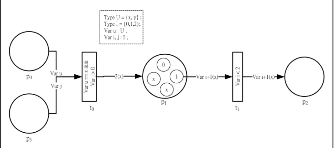
This section applies the CPNet (named as net and shown in Figure 2.2 ),

designed with four places, two transitions and four tokens, to explain how a CPNet works. The value of a U-type token located in place p is ₀ x and the value of I-type

tokens located in place p is ₁ 0 and 1 and in place p is 1 . The value fields of U ₃

and I data type are

{ }

x y, and

{

0,1, 2 , respectively.

}

Figure 2.2 An example of CPNet.

Definition 2.6 (Coloured Petri Nets – CPNets)

A Coloured Petri Net is a 9‐tuple CNet=( , , , , , , , ,P T F Σ C V A G m0) where

1. _{P is a finite set of places,} 2. _{T is a finite set of transitions,}

3. F is a finite set of directed arcs, F⊆

(

P∪ × ∪T

) (

P T

)

, satisfying

(

)

(

)

F∩ × = ∩ ×P P F T T =φ,

4. ∑ is a finite set of non-empty types, called color sets,

5. C is a color function, C P: →2∑, defined from _{P into the power set of} ∑ ,

6. V is a finite set of variables declared by the types in ∑ ,

7. A is an arc expression function, A F →: exp such that

(25)

( )

(

)

(

( )

)

(

)

: ( )

f F ⎡Var A f Type Var A f C p f ⎤

∀ ∈ _⎣ ⊆ ∑∧ ⊆ _⎦ 1

. 8. G is a guard function, G T →: exp such that ∀ ∈t T

(1) Type G t

(

( )

)

=Boolean 2 , (2) Var G t ⊆ ∑ ,

(

( )

)

(3)

(

( )

)

(

( )

,

)

p t Var G t Var A p t • ∈ =

_∪

and (4) p p1, 2 t Var A p t,

(

1,

)

Var A p t

(

2,

)

φ • ∀ ∈ ∩ = .

9. m is an initialization function, ₀ m P →0: exp, i.e., ∀ ∈ , p P m p0

( )

can

be represented with a multi-set3 over VE , defined below. By taking a _p

type c C p∈

( )

, a value element associated with p is a pair

(

c,val

)

where val is one of the colors in color set c. The set of all value elements of p is denoted by VEp=

{

(

c,val | c C p

)

∈

( )

∧val c∈ .

}

The data types associated with a place p are defined as a place color domain,

denoted as C p

( )

. The place color domains of net are C p

( ) { }

0 = U , C p

( ) { }

1 = U I, ,

( ) { }

2 ,

C p = U I and C p

( ) {}

₃ = I . All place color domains of a CPNet are included in ∑ . The tokens defined with given types included in C p

( )

are the tokens allowing to access p only. A transition t in a CPNet is considered as a procedure with a

1

The place connected by arc _f is denoted as _{p f}( ).

2

The data type of the value returned by evaluating an expression _exp is denoted as _Type(_exp). The set of

variables in _exp is denoted by _Var(_exp). The set of variable types used in the expression is denoted by

( )

(

exp

)

Type Var .

3

A multi-set m, over a non-empty set S, is a function _{m : S →} . The integer _{m s ∈}( ) is the number of

(26)

pre-condition, declared by a guard expression, denoted as G t

( )

. The variables associated with the expression of t are defined in its transition variable domain,

denoted as Var G t . In net , the transition variable domains of

(

( )

)

t0 and t1 are

{ }

u j, and

{}

i , respectively. In addition, each variable in Var G t is adopted once

(

( )

)

in one of t ’s input arc expressions, e.g., in net , the variable u is used in t ’s input ₀

arc expression, A p t

(

₀, ₀

)

=var u , only. For a variable v adopted in an arc

expression A p t

( )

, , Type v

( )

needs to include in C p

( )

.

Assigning the variables of a transition _{t with values is called transition binding,} defined in Definition 2.7. All bindings satisfying t ’s guard expression are stored in

( )

B t . The form of binding b can be represented as

1 1 2 2 n n

b= v =val ,v =val ,...,v =val where v is assigned with value _i val , _i

( )

(

)

{

_i|1

}

Var G t = v ≤ ≤i n . In net , there are two bindings b1= =i 3 and

2 5

b = =i in B t

( )

₁ .

Definition 2.7 (Transition Binding)

A binding of a transition _{t is a function}b Var G t:

(

( )

)

→ , M is defined M

in Definition 2.8, where ∀ ∈v Var G t

(

( )

)

1. b v

( )

=1

(

p c val, ,

(

)

, i.e., the value val of the c-typed token in p is

assigned to variable v in A p,t

( )

and replaces v of G t

( )

, and

2. Type v

( )

=c, i.e., the type of variable v is the same as that of the selected

(27)

A token element is a pair

(

p, c,val where p P

(

)

∈ and

(

c,val

)

∈VE_p, while a

binding element is a pair

( )

t,b where t T∈ and b B t∈

( )

. The set of all token elements of a CPNet is denoted by TE while the set of all binding elements is

denoted by BE . In net , the color sets associated with p and 1 p are U and I 2

while p and ₀ p are associated with U and I , respectively. The 3 TE of net is

composed of the token elements in the two sets,

( )

(

)

(

( )

)

(

)

{

p, U,x , p, U,y | p= p | p | p0 1 2

}

and

( )

(

)

(

( )

)

(

( )

)

(

)

{

p, I,0 , p, I,1 , p, I,2 | p= p | p | p1 2 3

}

.

The BE are

(

t ,b0 0

)

,

(

t ,b1 1

)

and

(

t ,b1 2

)

where b0= =u x,j=1 , b1= =i 0

and b₂= =i 1 .

Definition 2.8 (Marking)

A marking _{M is a multi-set over TE while a step Y is a non-empty and} finite multi-set over BE . The initial marking M is obtained by initialization 0

function m : 0

(

)

(

p, c,val

)

TE : M p, c,val0

(

)

(

m p0

( )

)

(

c,val .

)

∀ ∈ =

The set of all markings and steps are denoted by _{M and Y , respectively.}

Definition 2.9 (Step Enabled)

A step Y is enabled in a marking M , obtained by a marking function m , if and only if the following property is satisfied:

( )

( )t ,b Y

( )

p P : A p,t b m p

∈

(28)

Let

( )

t,b ∈Y. The tokens in A p,t b

( )

, a multi-set over VE yielded by the _p

arc expression A p,t

( )

upon b, are removed from p when t is fired with

binding b. By taking all binding elements

( )

t,b ∈Y, the tokens in the union of multi-sets generated by these binding elements are removed from the input places concurrently when _{Y occurs. Each binding element}

( )

t,b in _{Y must be able to get} the tokens specified by A p,t b

( )

, without having to share these tokens with other binding elements of Y .

Let step _{Y be enabled in the marking M . When}

( )

t,b ∈Y, _{t is enabled in M} with the binding b. If

(

t ,b , t ,b₁ ₁

) (

₂ ₂

)

∈Y and

(

t₁≠t₂

) (

∧ b₁≠b₂

)

,

(

t ,b₁ ₁

)

and

(

t ,b2 2

)

are enabled concurrently in marking M . If Y t ≥

( )

2 , i.e., ∃ i,j

( )

t,b , t,bi

( )

j ∈ and i may be j , t is enabled more than one time concurrently. Y

Definition 2.10 (Fire a Step)

When a step Y is enabled in a marking M , generated by marking function 1 1

m , marking function m generating the next marking 2 M from 2 M can be 1

defined as:

( )

( ) ( )

( )

2 1 t ,b Y t ,b Y p P : m p m p A p,t b A t,p b ∈ ∈ ⎞ ⎛ ∀ ∈ =_⎜⎜ − ⎟_⎟+ ⎝

∑

⎠

∑

Multi-set

( )

( )t ,b Y A p,t b ∈

∑

represents the tokens removed from p , while

( )

( )t ,b Y

A t,p b

∈

∑

denotes the tokens added to p . M is directly reachable from 2 1

(29)

The initial marking M₀ , generated by m₀ , of net is

( )

(

0

)

(

1

( )

)

(

1

( )

)

(

3

( )

)

1' p , U,x +1' p , I,0 +1' p , I,1 +1' p , I,1 . Let two sequential steps Y and ₁

2

Y be

{

(

t ,b0 0

)

}

and

{

(

t ,b , t ,b1 1

) (

1 2

)

}

. Before executing Y , the values of the tokens, 1

( )

(

0

)

1' p , U,x and 1' p , I,

(

3

( )

1

)

, are assigned to variable u and j upon

0 1

b = =u x,j= for evaluation, i.e., u is assigned with x of the token in place p , 0

while j is assigned with value 1 of the token in place p . In this case, the 3

evaluation result is true, hence Y is enabled in ₁ M and it may be fired. When 0 Y is 1

fired, one U-type token with value x and one I-type token with value 1 are

removed from p and ₀ p , respectively, and two U-type tokens with value 3 x are

added into p . The result is shown in Figure 2.3. ₁

In Y , transition ₂ t is enabled twice concurrently by binding 1 b1= =i 0 and

2 1

b = =i , i.e., the two binding elements in Y are able to remove the ₂

corresponding tokens, expressed as 1' p , U,x

(

₁

( )

)

+1' p , I,

(

₁

( )

0

)

and

( )

(

1

)

(

1

( )

)

1' p , U,x +1' p , I,1 respectively, from p at the same time. ₁

Figure 2.3 The result net of firing step Y . ₁

Var u _2(x)

Var i+1(x) Var i+1(x)

p0 p1 p2 t0 t1 Type U = {x, y} ; Type I = {0,1,2}; Var u : U ; Var i, j : I ; x 0 1 p3 Var j x

(30)

The definition of occurrence sequence of CPNets, omitted here, is similar to that of PNets, given in Definition 2.5.

2.3. Time Coloured Petri Nets — TCPNets

CPNets with timing constraints can be classified according to the ways of specifying timing constraints, a timing interval [16][17][23] or a specific time [18], or the elements of the net, place [19] , transition [16][18] and arc [15][20], these constraints are associated with. When timing constraints are associated with a transition, the constraint can be interpreted as (1) a delay time [18] [23], i.e., when the transition is fired, its input tokens are removed, but the output tokens is created until the delay time associated with the transition has elapsed, (2) a holding duration [21], i.e., when the transition is fired, its input and output tokens are removed and added concurrently, but the succeeding transition is enabled when the token created time within the holding duration denoted and (3) an firing interval [16][23], i.e., the transition can be fired in its firing interval only. For such transition, the mechanism of removing and adding tokens is the same as that of a transition associated with a delay time.

A common approach [23] is to associate a time stamp, denoted as @r , r∈ ,

with token, and attach a restricted firing interval, denoted as

[

min,max ,

]

min,max∈ , with transition. The transition output arc(s) can associate with a time requirement Δt to denote how many time units an execution of the transition takes. When a token is associated with a time stamp, the token is timed. If the time stamp is @r , the token is available to consume after r , i.e., r is the earliest time at

which the token can be used. Otherwise, the token is untimed and always ready to be used. For a timed transition t , there is a restricted firing interval

[

min,max

]

(31)

maximum firing time, respectively, i.e., t can be fired between min and max

only. In addition, an execution of t takes Δt time units which is equal to or more than 0. Δt is specified in t ’s output arc expression(s). An untimed transition,

defined without restricted firing interval, can be fired when it is enabled. The firing mechanism of untimed transition is the same as that defined in CPNets.

In a TCPNet, timed CPNet, a global clock is introduced. Let an activity, associated with a restricted firing interval

[

min,max , be presented with a transition

]

t in the net and t be fired at τ , min≤ ≤τ max. An execution of t takes Δt time units. The value of the time stamp(s) associated with the token(s), which will be removed from t ’s input place(s) when t is fired, needs to be less than τ . When t

is fired,

t creates a time stamp τ+Δt for its output token(s). Definition 2.11 (Timed Coloured Petri Nets)

A Timed Coloured Petri Net is a 5-tuple TNet=

(

CNet,I ,I ,R,r_INT _R ₀

)

where 1. CNet=( , , , , , , , ,P T F ΣV C G A m₀) is a CPNet where

(1) Σ = Σ ∪ Σ , i.e., the colour sets (types) in Σ can be divided into two _U _T disjoint sets, Σ and _U Σ . The elements in _T Σ are untimed and the _U elements in Σ are timed, i.e., a token typed with _T c ∈Σ is associated _T

with a time stamp,

(2) ∀ ∈ , the variables f F Var A f

(

( )

)

used in arc f are timed/untimed over

the timed/untimed subset of C p f and

(

( )

)

(3) ∀ ∈ , p P m p0

( )

generates a timed/untimed multi-set over the

timed/untimed subset of C p

( )

. The details are given in Definition 2.12. 2. I is an interval function _INT IINT:T→INT where INT=

{

[ , ]x y ∈ × |x y≤

}

.

(32)

For a transition t , t T∈ , the function assigns a firing interval

[

min,max .

]

3. I is a time function _R I FR: → where R R= Δ ∈

{

t |Δ ≥t 0

}

. For an arc

( )

t,p ,

( )

t,p ∈F, the function assigns the time units consumed by executing

t on

( )

t,p .

4. R , R ⊂ , is a set of time values, called time stamps. 5. r , ₀ r0∈ , is the start time. R

The definitions of the set of transition bindings B t

( )

, token elements TE ,

binding elements BE and step Y are the same as those of CPNets.

This section applies the TCPNet net (shown in Figure 2.4), designed with four

timed tokens and two timed transitions, to explain how a TCPNet works. We declare that R includes time stamps 100, 200 and 220. There are four tokens typed with the

colour sets in Σ , Σ = Σ . The U -typed token, which is assigned with value x and _T located in place p , is available after time 100. The three I -typed tokens, which are ₀

assigned with value 0, 1, 1 and located in place p , ₁ p , 1 p , are available at 100, 3

respectively. Transition t and ₀ t are associated with restricted firing intervals 1

[

180 220,

]

and

[

200 250,

]

, respectively. An execution of t /₀ t takes 20/30 time units. 1

Figure 2.4 Introducing time constraints into the CPNet shown in Figure 2.1.

(33)

Definition 2.12 (Timed Multi-set)

A timed multi-set tm , over VE of a place p p in CNet , is a function

p tm : VE × → , such that R 1. ₍_{c ,val}₎

(

)

r R tm tm c,val ,r ∈

=

∑

, an non-negative integer, denotes the number of

c-typed tokens associated with val in p ,

2. the time stamps associated with these c-typed tokens are listed in

(

)

1 2 i tm₍_{c ,val}₎

tm c,val⎡_⎣ ⎤_{⎦ ⎣}=⎡r ,r ,...,r ,...,r ⎤_⎦

where the time value r for _i tm c,val ,r ≠ ,

(

)

_i

)

0 1≤ ≤i tm₍_{c ,val}₎, are listed. r_i

appears tm c,val ,r times in the list and

(

)

_i

)

tm c,val⎡_⎣

(

)

⎤_{⎦ is sorted, i.e.,}

1 i i r r≤ + , 1≤ ≤i tm₍c ,val₎. A formal presentation of tm of p is ₍ ₎

(

)

( ) p

(

)

c ,val c ,val VE tm ' c,val @tm c,val ∈ ⎡ ⎤ ⎣ ⎦

∑

.

In net , formal presentations of the tokens located in place p , 0 p , 1 p are 3

( )

[ ]

1' U,x @100 , 1' I, @

( )

0

[ ] ( ) [ ]

100 +1' I, @1 100 and 1' I, @

( )

1

[ ]

100 , respectively.

Definition 2.13 (Timed Marking)

Given a Timed CPNet TNet=

(

)

, a timed marking (state) of

TNet can be denoted by a pair

(

M,r

)

, the untimed marking M is a multi-set

over TE of CNet and generated by marking function m at time r such that

(

)

(

p, c,val

)

TE : M p, c,val

(

)

_r

(

m p

( )

_r

)

(

c,val

)

∀ ∈ = .

The initial timed marking can be denoted by a pair

(

M ,r₀ ₀

)

. The sets of all untimed and timed markings are denoted by MU and MT, respectively.

(34)

Upon Definition 2.13, the initial timed marking

(

M ,r₀ ₀

)

of net is

( )

(

)

(

( )

)

(

( )

)

(

( )

)

(

1' p , U,x0 +1' p , I,1 0 +1' p , I,1 1 +1' p , I,3 1 ,@100

)

where

( )

(

)

(

( )

)

(

( )

)

(

( )

)

0 1 0 1 1 0 1 1 1 1 3 1 M = ' p , U,x + ' p , I, + ' p , I, + ' p , I, and r =₀ 100.

Definition 2.14 (Step Enabled)

Given a Timed CPNet TNet=

(

)

, a step Y of TNet is enabled in a timed marking

(

M ,r₁ ₁

)

at time r if and only if the following ₂

properties are satisfied:

(1)

( )

( ) r2 1

( )

t ,b Y p P : A p,t b m p ∈ ∀ ∈

∑

⊆ , (2) r₁≤ , r₂

(3) r is the smallest value of R which satisfies (1) and (2). 2

Let step Y of TNet be enabled in

(

M ,r1 1

)

at the smallest time r in R , 2 1 2

r ≤ . For each binding element r

( )

t,b ∈Y, the tokens in A p,t b

( )

, a multi-set over

p

VE yielded by the arc expression A p,t

( )

upon b at time r , are associated with ₂

time stamps whose values are equal to or smaller than r . ₁

The set of time stamps of net , marked with

(

M ,r0 0

)

where r =0 100, is

{

100 200 220

}

R= , , . Let two sequential steps Y and ₁ Y of net be 2

{

(

t ,b0 0

)

}

and

(

) (

)

{

t ,b , t ,b1 1 1 2

}

. The two steps are enabled at r and 1 r , respectively. The restricted 2

firing intervals of transition t and ₀ t are 1

[

180 220,

]

and

[

200 250,

]

. In Section 0,

the two sequential steps can be fired sequentially without concerning time constrains. Here, we concern the firing intervals of transition t and ₀ t . 1

(35)

For the case of Y , ₁ Y is enabled when 1 r =1 200 only, because ‘200’ is the only

time stamp in R between firing boundary 180 and 220 of t . If 0 Y is fired at 1 τ1,

1

200≤ ≤τ 220, one U-type token with value x and one I-type token with value 1

are removed from p and ₀ p , respectively, and two U-type tokens with value 3 x

are added into p . A time stamp ₁ @τ1+20 is created for the two added tokens. The

timed marking of the result net, shown in Figure 2.5, is

( )

(

1

)

(

1

( )

)

(

1

( )

)

1

1' p , I,0 @100 1+ ' p , I,1 @100 2+ ' p , U,x @τ +20. After firing _{Y ,}₁ Y can ₂

be enabled at r =₂ 220, if τ₁+20 220≤ . For the case of Y , ₂ Y can be enabled 2

when τ1=200 only. If Y is fired at 2 τ2=220, the two binding elements

(

t ,b1 1

)

and

(

t ,b1 2

)

in Y are able to remove the corresponding tokens, expressed as 2

( )

(

1

)

(

1

( )

)

1' p , U,x @220 1+ ' p , I,0 @100 and 1' p , U,x @

(

1

( )

)

220 1+ ' p , I,

(

1

( )

1

)

@100

respectively, from p at the same time. A time stamp ₁ @220 30+ is created for the four tokens generated by t and added into ₁ p . 2

Figure 2.5 The result net of firing step Y . ₁

(36)

Definition 2.15 (Fire a Step)

When a step Y is enabled in a timed marking

(

M ,r1 1

)

at time r , generated 2

by marking function m , marking function 1 m generating the next marking 2

(

M ,r2 2

)

from

(

M ,r1 1

)

can be defined as:

( )

( ) 2 ( )

( )

2 2 1 _r _r t ,b Y t ,b Y p P : m p m p A p,t b A t,p b ∈ ∈ ⎞ ⎛ ∀ ∈ =_⎜⎜ − ⎟_⎟+ ⎝

∑

⎠

∑

Multi-set

( )

( ) r2 t ,b Y A p,t b ∈

∑

represents the tokens removed from p , while

( )

( ) r2

t ,b Y

A t,p b

∈

∑

denotes the tokens added to p .

(

M ,r2 2

)

is directly reachable

from

(

M ,r₁ ₁

)

by the occurrence of the step Y , denoted as

(

M ,r1 1

)

⎡⎣Y,r2>

(

M ,r2 2

)

.

2.4. Timed CPNets with Hierarchy –H PNets T_C

A H PNet defined in Definition 2.16 is a Timed CPNet with hierarchy, which is _CT

defined as the followings:

1. Hierarchical Transition: A transition _{t in a}H PNet can denote a collapsed T_C

sub-process whose expansion is another H PNet. The pre-condition associated _CT

with _{t has to be met before the execution of t ’s corresponding net.}

2. Hierarchical Token: Each token in a H PNet is typed with a Petri net PNet , T_C

called PNet type, accompanied an initiation marking M . The set of markings ₀

0

(37)

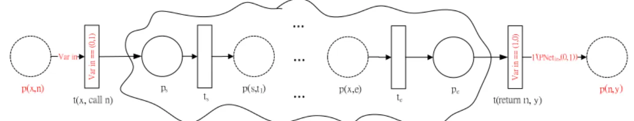
V ar in == ( 1,0) Var in 1'(0,1) @+20 p0 p1 t0[0,30]

Type PNet = {(0,1),(1,0)} timed; Var in : PNet ;

Global clock : 100 time units/cycle

(1,0) 1'(0,1) 1'(0,1)

p2

t1[50,100]

((PNet,(1,0))@10)

(a) An example of H PNet. _CT

(b) The design of PNet . (c) The H PNet T_C net' of compound transitiont .₀

Figure 2.6 An example of H PNet.T_C

This section applies the H PNet _CT net , shown in Figure 2.6 (a), designed with

three places and two transitions, to explain how a H PNet works. Let the initial T_C

marking of net be 1' p , PNet,

(

0

(

( )

1,0

)

@

[ ]

10 and transition t be compound. A 0

PNet -type token is putted in place p of net at time 10. The token is marked with 0

( )

1,0 while the place array of PNet is

(

p ,pa b

)

. The compound transition t can 0

be expanded to net', shown in Figure 2.6 (c).

Definition 2.16 (Hierarchical Timed Petri Nets – H PNets) T_C

(38)

(

)

HNet= TNet,TrSet,TkSet,TrFun,TkFun where

1. TNet=

(

)

is a Timed CPNet, where the set of transitions T in

0

( , , , , , , , , )

CNet= P T F Σ C V A G m can be divided into two disjoint sets, T and _A

C

T . The transitions in T are atomic and the transitions in A T are C

compound.

2. TrSet is a finite set of T C

H PNets each of which represents the expansion of a

compound transition in T . _C

3. TkSet is a finite set of PNets each of which represents the design of a data

type in ∑ .

4. TrFun is a compound transition mapping function, TrFun T: C →TrSet ,

defined from T to TrSet , TNet TrSet_C ∉ . The number of nets in set TrSet

is equal to the number of compound transitions in set T , i.e., _C TrSet = TC

and T ≥_C 0. Each compound transition in T is mapped into one of the _C

T C

H PNets in TrSet . Function TrFun is 1-1 and onto.

5. TkFun is a type mapping function, TkFun:∑ →TkSet, defined from ∑

into TkSet. The number of nets in set TkSet is equal to the number of types in ∑ , i.e., TkSet = ∑ and ∑ ≥0. Each type (color set) in ∑ is mapped into one of the PNets in TkSet. Function TkFun is 1-1 and onto.

Definition 2.17 (Weakly Connected Net)

A net, PNet or its extension, is called weakly connected if and only if replacing all of its directed arcs with undirected ones produces a connected net, i.e., there is a path between any pair of distinct nodes in the net at least.

(39)

Definition 2.18 (H PNet of Compound Transition) T_C

Given two weakly connected H PNets, HNet and _CT HNet', HNet HNet'≠ , a compound transition t of HNet is associated with HNet', TrFun t

( )

=HNet', if and only if the following conditions hold. Let CNet' of HNet' be composed of

0 '

( ', ', ', ', ', ', ', ',P T F Σ V C G A m ).

1. The input and output places of t are transferred into P' ,

( )

(

In t ∪Out t

)

⊂ , i.e., P' HNet' is started from the places in In t

( )

and terminated at the places in Out t

( )

. There is a path between any pair of start and terminated nodes at least,

2. T >' 1, the number of transitions in T' is more than 1,

3.

( )

( ) ( ) ' p In t Out t C p ∈ ∪ ⊆ ∑

∪

, the types (color sets) associated with the places in

( )

In t ∪Out t are included in ∑ and '

4. ∀ ∈p

(

In t

( )

∪Out t

( )

)

, C p'

( ) ( )

=C p , i.e., the types associated with p in HNet are the same as that in HNet'.

Definition 2.19 (PNet of Color Set)

Given a H PNet HNet and a weekly connected Petri Net _CT PNet=

(

P,T ,F ,m0

)

,

a type (color set) tp involved in HNet is designed with PNet , i.e.,

( )

TkFun tp =PNet, if and only if the following conditions hold:

(40)

2. ∀ ∈t T, 1|•t| |= t•|= , i.e., t has exact one input and output places, 3. The initial marking function m : P0 →

{ }

0 1, and 0

( )

1

p P

m p

∈

=

∑

, i.e., an initial marking M of PNet , generated by function 0 m , includes one token only. 0

From M₀ , all reachable markings include one token also,

[

0

( )

1 i i p P M M : m p ∈ ∀ ∈

∑

= , 0< ≤i n and n=

[

M₀

The number of colors in color set tp is less than or equal to the number of

places in PNet . These colors are presented with the states in

[

M0 .

For simplicity, and without losing generality, we assume that each H PNet has T_C

two levels in its hierarchy only. When a H PNet is designed with more than two _CT

levels, the compound transitions located in higher levels, 2 or more than 2, can be recursively replaced by its finer nets. In addition, any H PNet, restricted to start and T_C

end with places, is weakly connected, i.e., there is a path between any pair of distinct nodes (places and transitions) in the net at least.

(41)

Chapter 3. Business Process Modeling

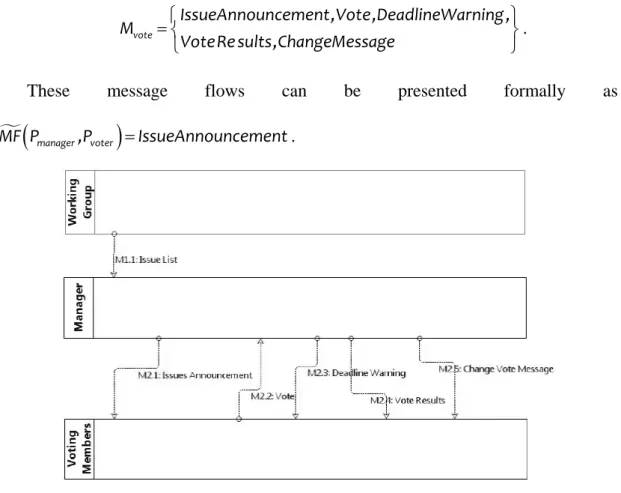
In general, a business process is implemented with one or more private processes (also called “process” in this thesis for short) for a business purpose. Each process is designed for a distinct business role (e.g., a buyer, seller, or manufacturer) or entity (e.g., a rule checking machine or banking system) involved. The participants acting the appointed roles cooperate according to the processes assigned to produce a product or service for a particular customer or market. Message sending is the only way to create a communication between processes. We define messaging as the (usually asynchronous) sending of a data item from a business role(s)/entity to other role/entity(ies). A message flow is used to present the transmission of messages. A business process specification, in Definition 3.1, defines the interactions between processes with message flow while the details of these processes are specified in their own specifications. The core modeling elements in BPMN are adopted and shown in Figure 3.1.

Definition 3.1. (Business Process Specification)

A business process specification is a 7-tuple BP (PP,A,M,MF ,MF ,PF ,P) , where =

1. PP is a set of private processes, as defined in Definition 3.2,

2. A denotes the set of artifacts used in BP ,

3. M denotes the set of messages used in BP ,

4. MF⊆

(

PP PP×

)

is a set of directed edges, called message flow, indicating the

(42)

5. MF : MF→M is a message function that maps each message flow into one of the messages in M ,

6. PF defines the set of resources that perform or are responsible for BP

7. P : PP→PF is a resource (onto) function that maps each process into one of

the resources in PF .

Figure 3.1 The core modeling elements in BPMN.

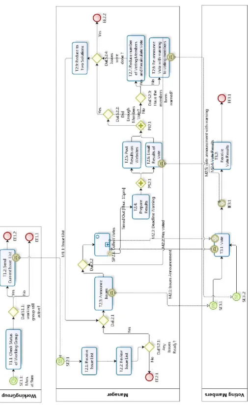
A business process for resolving problem through e-mail votes is applied in this thesis for demonstrating the usage of our formal model. The example is illustrated from broad to narrow.

There are three roles, working group, manager and voter, responsible for the voting business process, BP_vote. The assignments of the three roles, process P_workingG,

manager

P and P_voter, are described within their own swimlanes. The control and data flows of the three processes are introduced in Section 3.2.4 and 3.3.4, respectively. The participants acting working group, manager or voter execute P_workingG, P_manager or

運用一具Hierarchy 特性的Timed CPNets 技術來分析BPMN 工作流程

國

立

交

通

大

學

資訊科學與工程研究所

博

士

論

文