財政政策與景氣波動：不完全競爭總體模型之分析

1

國立臺灣大學社會科學院經濟學系 博士論文

Department of Economics College of Social Sciences

National Taiwan University Doctoral Dissertation

財政政策與景氣波動：不完全競爭總體模型之分析 Fiscal Policy and Business Cycles: An Analysis of

Imperfectly Competitive Macroeconomic Model

張振維

Cheng-Wei Chang

指導教授﹕賴景昌 博士 Advisor: Ching-Chong Lai, Ph.D.

中華民國 101 年 7 月

July, 2012

ii

謝辭

自 2006 年 9 月進入台大經濟研究所迄今，時光匆匆的過了六個寒暑春秋。

在這六年的歲月裡，儘管忙碌地埋首研究，日子卻過得相當充實，並且順利地完 成了博士論文。回憶這六年來的點點滴滴，雖然過程是如此崎嶇難行，沒有半點 燈光，但卻在蛻變後才發現，人生的挫折是讓自己茁壯的試金石，所以要化悲憤 為力量，這樣方能從經驗與教訓中吸取成長的養分。

首先，我要感謝指導教授 賴景昌老師願意指導我這個資質駑鈍的學生，讓 我領略到學術的浩瀚與嚴謹。對我而言，老師就像一盞明燈，以循循善誘的教導 方式，教導我如何在漫無邊際的學術範疇中找到定位，並在論文無解之處，巧妙 的銜接可能找到答案的地方，使得論文得以完成；在日常生活中，一方面，關心 學生的經濟狀況，讓我得以專心於學術研究，另一方面，教導學生待人處事的原 則，勉勵我懷著同理心學習對待人事物，以及對社會的關懷。

此外，我非常感謝張俊仁老師、陳明郎老師、陳南光老師、洪福聲老師、金 志婷老師，他們仔細閱讀我的論文，並在宏觀的高度上給予諸多非常寶貴的意 見，使得本論文臻至完善。正因如此，本論文若能對學術界有所貢獻，我的恩師 賴景昌老師與各位老師都居功厥偉。我真心地感謝黃俊傑老師平日的關照與鼓 勵，讓我在博士班的日子裡，得以無憂地堅持住對學術的研究與對熱情。我感謝 蔡雪芳老師對我的鼓勵與教導，至今我仍感念於心。我非常感謝曹添旺老師願意 幫我寫推薦信申請中研院博士候選人培育計畫。我也感謝當初鼓勵與支持我尋找 研究方向的老師，我會永遠珍藏在心中。

在台大與中研院學習的這段時間，感謝廖志興學長、朱巡與陳冠任等先進對 論文所提供的諸多寶貴意見，感謝李國豪學長在我論文沒有任何頭緒之際，教我 如何「單點突破」，感謝廖先昱樂於一起討論與解決在研究上所遇到的問題，感 謝曾憲政學長、陳映安學姐與謝惠婷在研究過程中所提供的寶貴意見，感謝楊禮 禎助教平日對我的照顧與幫助。

謝謝祥玲的支持與鼓勵，在我多次徬徨與無助的時刻，給我面對挫折的勇 氣，讓我在失敗中重新思考整頓我的思緒。感謝這一路上相信我與支持我的朋 友，謝謝你們在我低潮時，與我分享你們人生的智慧與經驗，以此來啟發我並鼓 勵我向前。

最後，我要誠摯地感謝我的父母，你們終日勞碌、不辭辛苦的工作，讓我自 由地去追逐我的夢想，如今，論文可以順利完成並取得博士學位都要歸功於你們 無私的付出。

博士論文的完成，代表著求學階段的結束，同時也象徵著另一階段的開始。

未來的旅程，我要告誡自己，必須不斷地吸收新知，並勉勵自己能將所學貢獻於 學術界與社會。

張振維 謹識 國立台灣大學經濟研究所 中華民國一百零一年八月

iv

摘要

總體經濟模型結合了不完全競爭的市場特性，為市場造成了扭曲。80 年中

期以後，「不完全競爭的總體經濟理論」發展至今多如恆河沙數，本篇論文試圖

將產業經濟的特質與市場的調整機制納入模型設定中，從新檢視不完全競爭的市 場特性將如何影響景氣波動與最適財政政策，希冀對不完全競爭的總體經濟模 型，有更深刻的了解與認識。

在第一篇文章，我們將不完全競爭的市場結構與傳統實質景氣循環模型結 合，並向兩個方向延伸：第一，我們結合產業經濟的觀點，考慮專業化分工是否 具有規模報酬的特性；第二，我們考慮進入成本的擁擠效果–在產業經濟研究 中，市場中既有的廠商家數越多，廠商的進入成本將越高，例如廣告成本。將這 兩種效果引入模型，我們發現，專業化分工的程度與進入成本的擁擠效果將左右 經濟體系複均衡的存在性。另外，專業化分工的效果支配著消費性政府支出對私 人消費與實質工資的影響。最後，考慮進入成本的擁擠效果，我們發現隨著政府 支出增加，個別廠商的生產將會提高，而並非一個常數。

在第二篇文章，我們假設個別廠商的生產技術具有規模報酬遞增的特性。另 外，依循公共財政學的觀點，我們將政府支出的生產性功能納入模型，同時也考 慮政府的生產性支出所衍生的擁擠效果。最後，為了充分了解獨占力指數與專業 化分工程度對經濟體系的影響效果，我們將獨占力指數與專業化分工程度用兩個 參數分別代表。在這個架構下，我們發現幾個結論。第一，經濟體系複均衡的存 在性與專業化分工程度有關但與獨占力指數無關。第二，在具有比例式相對擁擠 效果下，政府的生產性支出彈性將無法左右經濟體系複均衡的存在。第三，個別 廠商規模報酬遞增的程度越大，則經濟體系越難出現複均衡現象。第四，我們以 實質景氣循環模型所採用的參數值進行分析，結果發現，在單純具有比例式絕對 擁擠效果情況下，資本產出彈性趨近於零，勞動產出彈性趨近於一，而這結果與

實證資料相吻合。

在第三篇文章，我們分析當市場同時存在消費外部性與生產外部性的情況 下，政府如何制定最適的財政政策。另外，我們亦考量生產專業化具有規模報酬 遞增的特性與個別廠商的生產技術具有規模報酬遞增的特性。藉由市場調整機制 的不同，我們發現幾個結論。第一，若政府同時具有消費稅與所得稅兩項政策工 具，則消費稅是用來矯正消費外部性最適的政策工具，而所得稅是用來矯正生產 外部性最適的政策工具。第二，最適所得稅的制定將會因市場調整機制的不同而 有所改變。第三，當市場中的廠商家數固定不變，則最適的政府支出佔所得的比 例將等於政府支出的生產彈性，相反的，當市場中的廠商家數可以自由調整，則 最適的政府支出佔所得的比例將不等於政府支出的生產彈性。第四，當生產專業 化具有規模報酬遞增而且報酬遞增的程度夠大，則市場自由進出之下所決定的廠 商家數有可能低於社會最適的廠商家數。

關鍵字：不完全競爭、複均衡、財政政策、外部性、景氣循環

vi

Abstract

When imperfect competition is introduced to a general equilibrium macroeconomic model, the market allocation mechanism ceases to be efficient.

Since the mid-1980s, there have been a vast number of articles that have been discussed in the context of imperfectly competitive macroeconomic models. This thesis attempts to introduce the features of both industry organization and adjustment mechanisms to our analysis, and in so doing reviews how the business fluctuations and government policies are affected by the imperfectly competitive market structure.

It is hoped that we can arrive at a better understanding of imperfectly competitive macroeconomic equilibrium models.

In the first essay, we introduce two features to our analysis. First, in line with the viewpoint of industry organization, we consider the feature of returns to production specialization. Second, we consider the congestion effect of the start-up cost. In the industry organization, the greater the number of firms, the greater is the cost of product differentiation. This implies that the cost of initial advertising to make consumers aware of a new brand is greater. By introducing these effects into our model, several main findings emerge from the analysis. First, we find that the necessary and sufficient condition for equilibrium indeterminacy is closely related to the extent of production specialization and the congestion effect of the start-up cost.

Second, the effects of government spending on consumption and real wages depend on the extent of production specialization. Third, the output level of an individual firm is positively related to fiscal expansions, provided that the congestion effect of the start-up cost exists.

In the second essay, we suppose that the production technology for individual

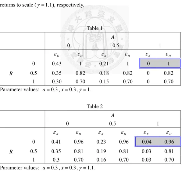
firms exhibits the feature of internal increasing returns to scale in imperfectly competitive industries. In line with the literature in the public finance field, we consider the role of productive government spending that is subject to the congestion effect. In addition, in order to clarify whether the crucial factor for the local indeterminacy is production specialization or monopoly power, we specify two distinct parameters to reflect the returns to production specialization and the degree of monopolistic competition. Equipped with these features, several interesting results are derived from our analysis. First, the necessary condition for equilibrium indeterminacy is independent of the monopoly power. Second, in the presence of proportional relative congestion, the equilibrium indeterminacy disappears even if productive government expenditures are incorporated. Third, when the production technology of a private firm possesses the feature of internal increasing returns, the possibility of the emergence of local indeterminacy is negatively related to the extent of the internal increasing returns to scale. Fourth, we adopt the parameters set in the existing RBC works, finding that under the situation where public services are subject to purely proportional absolute congestion, the output elasticity of capital is close to zero and the output elasticity of labor is close to one. This result is consistent with the empirical findings.

In the third essay, we analyze the optimal fiscal policies in the presence of consumption and production externalities and consider both the role of the extent of increasing returns to specialization and the role of internal increasing returns to scale.

By introducing three differential types of adjustment mechanisms, several main findings emerge. First, if both consumption and income taxes are available to the government, the consumption tax should be utilized to correct consumption externalities and the income tax should be utilized to remedy production externalities.

Second, the inclusion of three different types of adjustment mechanism plays an

viii

important role in governing the implementation of optimal income taxes. Third, the optimal ratio of government expenditure is solely determined by the extent of production externalities if the number of firms is constant, while the result should be modified if the free entry and exit of firms is brought into the picture. Fourth, free entry in the competitive equilibrium may result in under entry, provided that the degree of increasing returns to specialization is sufficiently strong.

Keywords: Imperfect competition; Indeterminacy; Fiscal policy; Externalities;

Business cycles

Content

口試委員會審定書………...………..…………i

謝辭………..…………ii

摘要………..…………iv

Abstract……….………..…………vi

1. Introduction………..…………1

2. The Effects of Government Spending with Free Entry………..10

2.1 Introduction………..………..10

2.2 The Model………..….12

2.2.1 Firms………...………..12

2.2.2 Households……….……..……….16

2.2.3 The government………..………..……….17

2.2.4 The competitive equilibrium………...……….18

2.3 Long-run effects of fiscal policy………..…………18

2.4 Conclusion………..………..…………27

3. Monopoly Power, Endogenous Entry, and Macroeconomic (In)Stability in a Growing Economy……….………28

3.1 Introduction………..……….28

3.2 The Model……….30

3.2.1 Firms………...……….31

3.2.2 Households……….……..……….35

3.2.3 The government………..………..……….37

3.2.4 The competitive equilibrium………...……….37

3.3 Macroeconomic Indeterminacy………..…………40

3.3.1 The condition for indeterminacy……….….41

x

3.3.2 Economic intuition for indeterminacy………..……….42

3.4 Conclusion……….…………..………..…………45

4. What Determines Optimal Fiscal Policies under Imperfect Competition? A Comprehensive Analysis………..………..………47

4.1 Introduction………..……….…………47

4.2 The Model……….50

4.2.1 Firms………...……….50

4.2.2 Households……….……..……….53

4.2.3 The government………..………..……….55

4.3 Optimal Fiscal Policies with Endogenous Number of Firms…………55

4.3.1 The decentralized equilibrium……….…………..……….….57

4.3.2 The centralized equilibrium………..……….….58

4.3.3 Optimal fiscal policies………..……….….59

4.4 Optimal Fiscal Policies with Endogenous Overhead Costs…………66

4.4.1 The decentralized equilibrium………….………..……….….67

4.4.2 The centralized equilibrium………..……….….….68

4.4.3 Optimal fiscal policies………...……….….68

4.5 Optimal Fiscal Policies with the Existence of Monopoly Profits……70

4.5.1 The decentralized equilibrium……….…………....……….….71

4.5.2 The centralized equilibrium………....……….….72

4.5.3 Optimal fiscal policies……….…….……….….72

4.6 Conclusion………..………..…………74

5. Conclusion……….……….…76

References………..………….………..…..………...…….…..…………79

Chapter 1

Introduction

Many recent studies in macroeconomics, such as Startz (1989), Rotemberg and Woodford (1992), Chang et al. (2007), Lai et al. (2010) and Bilbiie et al. (2012), to mention just a few, have focused on macroeconomic policies in the presence of imperfect competition. As this literature has developed, it has become clear that the degree of monopoly power (the price markup) in the analysis crucially governs the results compared to the perfect competition. Under imperfect competition, all firms set a price as a markup over marginal cost and, as a result, enjoy non-negative profits, provided that the number of firms is given exogenously. However, if we relax the assumption that the number of firms is fixed, the model itself instead endogenously determines the equilibrium number of firms by the zero-profit condition due to free entry.

In an influential paper, Startz (1989) shows that a higher degree of monopoly power tends to result in more profits and hence increase the households’ disposable income. As a result, the degree of monopoly power can govern the transitional dynamics of the economy by way of this so-called feedback effect. Once free entry is allowed, it will result in zero profits in equilibrium and, of course, cut off the feedback effect from monopoly profits. This prompts Startz (1989) to conclude that the short-run output multiplier exceeds the long-run multiplier. By endogenizing the number of firms, Devereux et al. (1996) introduce both imperfect competition and increasing returns to production specialization to the real business cycle (RBC) model.

Based on this framework, they obtain two important results. First, “the impact of

government spending on long-run consumption [crucially] depends not only on the markup, but also on the [labor supply elasticity] (p. 244).” Second, fiscal spending may raise private consumption, provided that the degree of monopoly power is large.

However, in their paper, the extent of monopoly power and the degree of increasing returns to specialization are governed by the same parameter. A question thus naturally arises in their analysis: Does the positive linkage between government spending and private consumption stem from the returns to production specialization or the degree of monopoly power? The first purpose of chapter 2 is to clarify which one is the key factor for the volatility of private consumption.

Empirical evidence on the co-movement between real wages and aggregate output are mixed. On the one hand, Solon et al. (1994) and Kandil (2005) find that real wages are strongly pro-cyclical in the U.S. On the other hand, Gärtner (2009) finds that Canadian real wages experience countercyclical behavior. However, the standard real business cycle models derive a result that a positive fiscal shock financed by a lump-sum tax leads to a fall in real wages. In other words, the co-movement between real wages and aggregate output could not be exhibited in the RBC framework. Thus, the second purpose of this chapter is to provide a new channel to reconcile the discrepancy from the empirical observations.

Furthermore, as stated by Devereux et al. (1996, p. 239), “with our specification, all variation in aggregate output is due to entry and exit, as output per firm is unaffected by changes in the aggregate state … [and] this implication is, of course, at odds with the fact that output per firm does vary over time.” However, empirical observation, such as that by Basu (1995), finds that “the quantities of intermediate goods used should be pro-cyclical.” Based on this cognition, the third purpose of this chapter is to bridge the discrepancy between the theoretical analysis and empirical evidence. That is, we provide a new channel to show that the output per firm is no

longer fixed in the long run.

It should be noted that the notion of production specialization originates from industry organization, namely, economies of scope. Economies of scope constitute an important issue in the production process in industry organization theory. As stated by Panzar and Willig (1981), “there are economies of scope where it is less costly to combine two or more product lines in one firm than to produce them separately..., and diseconomies of scope if the [situation] is reversed.” Based on this, in chapter 2, we make a distinction between production specialization and monopoly power and specify a generalized specification of production specialization to capture the observations in the industry organization. Furthermore, as stated by Das and Das (1996, p. 218), “[entry] costs would arise .... An example would be the cost of initial advertising to make consumers aware of a new brand. The greater the number of entrants the greater is the cost of product differentiation.” Therefore, in line with Das and Das (1996), Kim (1997) and Chen et al. (2005), our model supposes that the start-up cost is positively related to the number of firms.

By introducing these features into our model, several main findings emerge from the analysis. First, we show that the necessary and sufficient condition for local indeterminacy is independent of the monopoly power but closely related to the degree of returns to specialization and the congestion effect of the start-up cost. Second, private consumption and the real wage are pro-cyclical in relation to aggregate output in the presence of increasing returns to specialization. By contrast, consumption and the real wage are counter-cyclical in relation to aggregate output in the presence of decreasing returns to specialization. Finally, output per firm will increase in response to an expansion in government spending, provided that the congestion effect of the start-up cost exists.

In an influential paper, Benhabib and Farmer (1994) show that if the production

function is featured with increasing returns to scale and the degree of the increasing returns is sufficiently strong, a self-fulfilling equilibrium driven by the agents’

optimistic expectations can be generated in a one-sector RBC model. However, the empirical evidence, such as Burnside (1996), suggests that private production externalities at the aggregate level are much smaller. Motivated by this counterfactual inconsistency in the literature, subsequent research over the last two decades has tended to proceed in two distinct directions. One line of research has incorporated several elements into the Benhabib and Farmer (1994) model in order to push down the required degree of increasing returns in order to generate local indeterminacy.¹ The other line of research has highlighted the importance of rules (regimes) to investigate the emergence of local indeterminacy.²

For example, by endogenizing the number of firms in the Benhabib and Farmer (1994) model, Chang et al. (2011) show that imperfect competition leads aggregation increasing returns to variety, which pushes down the required degree of increasing returns for generating local indeterminacy. However, it is worth noting that although the work done by Chang et al. (2011) is valuable, they assume that the extent of monopoly power and the degree of returns to specialization are governed by the same parameter. As such, it is inconvenient for us to precisely understand which one is the key factor for the equilibrium indeterminacy condition. Thus, by making a distinction between returns to specialization and monopoly power, one purpose of this chapter is inclined to clarify whether the crucial factor for the local indeterminacy is production specialization or monopoly power.

Besides, Guo and Harrison (2008) make an attempt to shed light on the

1 See also, for example, Wen (1998, 2008), Chang et al. (2011) and Chen and Zhang (2011), among others.

2 See also, for example, Schmitt-Grohé and Uribe (1997), Guo and Harrison (2004, 2008) and Chin et al. (2009), among others.

importance of productive public expenditures in governing the dynamic behavior of the economy. However, in their framework they only consider a special case of the pure public goods. As claimed by Thompson (1974) and Barro and Sala-i-Martin (1992), all publicly provided services, such as transport, public utilities and possibly national defense, are characterized by some degree of congestion. This motivates us to take the congestion effect into account to test whether the result in Guo and Harrison (2008) still holds.

Some existing RBC studies find a puzzling fact: capital services seem to play no role in explaining cyclical fluctuations in output while the estimated labor output elasticity exceeds one.³ Based on this, Wen (1998) incorporates capacity utilization into the standard real business cycle model with production externalities and thus provides a possible explanation for this empirical puzzle. With the channel of the productive government spending that is subject to the congestion effect, this paper tries to provide a new channel to solve the puzzle.

By using firm-level panel data, Chirinko and Fazzari (1994) suggest that the production technologies for the competitive firms are increasing returns in imperfectly competitive industries. The theoretical studies, such as Ambler and Cardia (1998), Weder (2000) and Dos Santos Ferreira and Lloyd-Braga (2008), focus attention on discussing the role of internal increasing returns to scale in relation to various topics.

Based on this, in chapter 3, we set up a monopolistically competitive model with internal increasing returns to scale. Besides, we extend not only the Chang et al.

(2011) model to make a distinction between returns to production specialization and monopoly power, but also the Guo and Harrison (2008) model to include the congestion effect stemming from government spending.

Equipped with these straightforward extensions, several interesting results are

3

derived from our analysis. First, under the scenario where public services are subject to purely proportional absolute congestion, the output elasticity of capital is close to zero and the output elasticity of labor is close to one. This result is confirmed by Wen (1998) who stresses that “the estimated capital elasticity is near zero and the estimated labor elasticity is near one.” Second, running in sharp contrast to the Chang et al. (2011) result, the necessary condition for equilibrium indeterminacy is independent of the extent of monopoly power. Besides, in the case of proportional relative congestion, the necessary condition for equilibrium indeterminacy is independent of the elasticity of the productive government expenditure. To be more specific, it is unlikely for a one-sector growth model with productive government spending to exhibit local indeterminacy, provided that proportional relative congestion exists. That is, the result in Guo and Harrison (2008) no longer holds. Finally, when the production technology in the private sector possesses the feature of internal increasing returns, the higher the degree of internal increasing returns, the more difficult it will be for the indeterminacy result to arise.

Since we have studied the positive analysis in previous chapters, it is natural to go further to investigate fiscal policy in order to remedy market imperfections and externalities, such as productive government spending, the congestion effect and the imperfectly competitive market that we have discussed in the previous section. The majority of existing studies concerning market externalities can generally be classified based on two aspects, namely, consumption externalities and production externalities.

With regard to consumption externalities, a number of studies, such as Ljungqvist and Uhlig (2000), Dupor and Liu (2003), Liu and Turnovsky (2005) and Liu and Chang (2011) have devoted considerable amounts of attention to implementing the optimal fiscal policy to correct consumption externalities. With regard to production externalities, Eicher and Turnovsky (2000), Gómez (2004), Chang et al. (2009) and

Lai and Liao (2012) have carefully examined the optimal fiscal policies in the model with production externalities.

Following Dixit and Stiglitz (1977) and Blanchard and Kiyotaki (1987), many recent studies instead focus on macroeconomic policies in the presence of imperfect competition. Up till now, three familiar but distinct types of mechanism have been discussed in the imperfect competition literature. One line of the literature allows positive profits in equilibrium to highlight the importance of monopoly profits available in the economy.⁴ By contrast, under imperfect competition with the free entry and exit of firms, another line derives the result that monopolistically competitive firms will make zero profits in equilibrium.⁵ Besides, the other line of the literature, in particular, utilizes the zero-profit condition to determine the overhead cost instead of the number of firms in equilibrium to emphasize the fact that the overhead cost is crucial to economic activities.⁶

Compared with the existing studies on normative analysis under imperfect competition, our analysis is characterized by three distinct traits. The first distinction is the introduction of internal increasing returns to scale stemming from diminishing marginal costs. Until now, the linkage between optimal fiscal policies and the extent of internal returns to scale has been virtually absent in the existing literature. This paper thus turns the focus to the extent of the internal returns to scale.

As we will show later, the extent of the internal returns to scale is a crucial determinant of the optimal fiscal policies. The second distinction is the simultaneous presence of consumption and production externalities. As such, once the consumption tax and income taxes (on both labor income and capital income) are

4 Of the various studies, Dixon (1987), Benhabib and Farmer (1994), Chang et al. (2009) and Lai et al.

(2010) focus on this situation.

5 Dixon and Lawler (1996), Devereux et al. (2000), Chang et al. (2011) and Bilbiie et al. (2012) deal with this situation.

6

available to the government, we will thus use it to compare the relative efficiency of fiscal policies between consumption externalities and production externalities.

According to our analysis, there exists an appropriate use of consumption tax and income tax for consumption and production externalities. The third distinction is the adjustment mechanism. The existing imperfect competition studies on the optimal fiscal policies are either characterized by a zero-profit condition due to free entry or, alternatively, adopt a constant number of firms in which there exist positive profits.

It has been well known that the introduction of fiscal policies can be utilized to remedy inefficiency in the presence of externalities. Owing to the fact that three differential types of mechanisms are being discussed in the imperfect competition literature, this paper thus introduces the adjustment mechanism to address the interrelations between the optimal fiscal policies and market distortions under different types of mechanisms. According to our analysis, the adjustment mechanism is a crucial determinant of the optimal fiscal policies in the presence of market distortions.

By introducing these features into our model, several main findings emerge.

First, in the presence of consumption and production externalities, a consumption tax should be utilized to correct consumption externalities, while an income tax should be utilized to remedy production externalities. Second, the inclusion of an adjustment mechanism plays an important role in governing the implementation of optimal labor and capital income taxes. Third, when the government spending provides productive services, the optimal ratio of government expenditure is solely determined by the extent of the production externalities if the number of firms is fixed, while the result should be modified if free entry and exit of firms is taken into account. Fourth, free entry in the competitive equilibrium may result in under entry, provided that the degree of increasing returns to specialization is strong enough.

The remainder of this dissertation is organized as follows. Chapter 2 examines the economic dynamics and the cyclical behavior of consumption and real wages in which a generalized specification of production specialization and the congestion effect of the start-up cost are taken into account. Chapter 3 focuses on the dynamic properties under the one-sector growth model in which we distinguish returns to specialization from monopoly power. Besides, we consider the role of the extent of internal increasing returns and the role of productive government spending that is subject to the congestion effect. Chapter 4 introduces three types of mechanism dealing with the optimal fiscal policies in the presence of consumption and production externalities. Finally, Chapter 5 concludes our analysis.

Chapter 2

The Effects of Government Spending with Free Entry

2.1 Introduction

According to the standard real business cycle (RBC) models with perfect competition and constant returns-to-scale technology, a positive fiscal shock financed by a lump-sum tax leads to a fall in both consumption and real wages.⁷ The reason for this result is that an expansion in fiscal spending generates a negative wealth effect, which leads to a reduction in private consumption and a rise in the level of labor supply (and hence employment), thereby resulting in a decrease in the real wage.

Accordingly, both real wages and consumption exhibit countercyclical behavior over the business cycle. However, in general the theoretical predictions concerning the behavior of both real wages and consumption from the standard RBC models are not consistent with the empirical evidence.

With regard to the cyclical behavior of real wages, existing empirical studies on the co-movement between real wages and aggregate output are mixed. On the one hand, using data from the U.S. economy, Solon and Barsky (1989), Solon et al.

(1994), Hart et al. (2002) and Kandil (2005) find that real wages are strongly pro-cyclical.⁸ On the other hand, Gärtner (2009) finds that Canadian real wages experience countercyclical behavior.⁹ However, the existing theoretical studies including Baxter and King (1993), Cardia (1995), Edelberg et al. (1999), Burnside et al. (2004) and Cavallo (2005) assert that real wages are countercyclical; that is, real wages are negatively correlated with aggregate output. Up till now, to the best of our knowledge, it is surprising that the economic modeling of the positive

7 See Rebelo (2005) for a survey on the properties of RBC models.

8 By taking job stayers into account, Shin and Shin (2008) obtain a similar result. Since job stayers constitute a major fraction of the labor force, their analysis constitutes important progress in understanding the procyclicality of real wages. See Shin and Shin (2008) for detailed discussions.

9 Throughout this chapter, that real wages are procyclical is defined to involve higher real wages in good times (output is rising), and that real wages are countercyclical is defined to involve lower real wages in good times. See, for example, Kaminsky et al. (2004) and Woo (2009).

relationship between real wages and aggregate output has been virtually absent in the literature. The first purpose of this chapter is thus to provide a plausible solution to reconcile the discrepancy between the theoretical prediction and empirical observations.

With reference to the cyclical behavior of consumption, empirical studies by Blanchard and Perotti (2002), Fatas and Mihov (2002), Gali et al. (2007) and Ravn et al. (2007) find that a fiscal expansion is associated with a rise in private consumption.

The conflict between theoretical inference and empirical observation is now dubbed

“the fiscal policy puzzle” in the literature. Recently, some studies have made an effort to provide their solution to the fiscal policy puzzle. Chen et al. (2005) first consider the productive role of government spending as a possible vehicle to explain the positive co-movement between consumption and fiscal spending. In addition, by specifying the non-separable utility function, Linnemann (2006) and Bilbiie (2009) solve the puzzle from the perspective of preference-based explanations. Devereux et al. (1996) show that in the presence of increasing returns to specialization stemming from monopoly power, a government spending shock can generate a positive response of private consumption if increasing returns are sufficiently large.

However, in their analysis they specify a parameter to capture both the returns to production specialization and the degree of monopolistic competition. A question thus naturally arises in their analysis: Does the positive linkage between government spending and private consumption stem from the returns to production specialization or the degree of monopolistic competition? The second purpose of this chapter is to clarify whether the key factor for the pro-cyclical behavior of private consumption is the returns to production specialization, rather than the degree of monopolistic competition. In addition, in Devereux et al. (1996), the production of each intermediate good remains intact and aggregate production is increased in response to an expansion in fiscal expenditure. This result, however, stands in stark contrast to the empirical observation. For example, Basu (1995) finds that the quantities of each intermediate good used should be pro-cyclical rather than fixed. To bridge the discrepancy between the theoretical analysis and empirical evidence, this chapter endogenizes the start-up cost that is subject to the congestion effect, and shows that the intermediate good production is no longer fixed in the long run.

The returns to production specialization are now regarded as an important factor

affecting the scale economies in the production of manufactures (Holtz-Eakin and Lovely, 1996). As documented by Francois (1990, p. 110), “[the] gains from [the returns to production specialization] are realized through the reorganization of the production process and through qualitative changes in the mix of inputs which, in turn, require increased use of management and highly specialized personnel.” Based on the above viewpoint observed in the industrial economy, this chapter develops a dynamic general equilibrium model featuring the returns to production specialization, and uses it to explore the relationships among real wages, consumption, and aggregate output.

The remainder of this chapter is organized as follows. Section 2 sets up a dynamic optimizing macro model which is able to capture both increasing and decreasing returns to specialization. Section 3 deals with how real wages and private consumption will react in response to an expansion in government spending.

Finally, concluding remarks are provided in Section 4.

2.2 The model

The economy we consider consists of three types of agents: households, firms, and a government. The production side of the economy consists of two sectors: the perfectly competitive final good sector and the monopolistically competitive intermediate goods sector. Suppose that the final good is produced through the use of a range of differentiated intermediate inputs. The households derive utility from the consumption of the final good and from enjoying leisure, and they accumulate physical capital as a saving asset. The government levies a lump-sum tax to finance its expenditures.

2.2.1 Firms

Following Bénassy (1998), final output is produced by perfectly competitive firms with the following technology:¹⁰

 

  ¹

0 1 1

) (





N  ^Ny_i di

Y ;01, 0, (1)

10 To simplify the notation, in what follows the time subscript of all variables is omitted except in cases where it should be brought to the reader’s attention.

where y represents the quantity of input _i i used in the production of the final good and N is the number of intermediate goods. As we will explain later, the parameter  measures the degree of monopoly of the intermediate good firms, and the parameter  measures the extent of the returns from specialization.

The production function reported in equation (1) displays a generalized form of increasing (or decreasing) returns to specialization in the sense that the larger the number N of intermediate firms, the higher (lower) the amount of final output obtained. If all intermediate goods are hired in the same quantity, namely, y , then final output is given by Y N^1y. Thus, there are constant returns to the quantity employed of a fixed variety of intermediate goods, but either increasing (if 0) or decreasing (if 0) returns to an expansion in variety, while holding fixed the quantity employed of each intermediate good.

In their paper, Devereux et al. (1996) and Chang et al. (2007) specify that the production function of final output has the following form: ^{ }

1

0 )

(



 ^Ny_i di

Y , where

monopoly power and increasing returns to specialization (an expansion in variety) are characterized by the same parameter  . As stressed by Bénassy (1998), the specification of equation (1) allows us to clearly separate increasing returns to specialization from monopoly power, so that both effects can be fully disentangled.

Assuming that the final good is the numéraire, the profit-maximization problem for the final good firm can be expressed as:





 ^{ N} _i ^N _{i i}

f

y N y di p y di

Max

i 0

1

0 1 1

)

( ^{ }

 

 ,

where p is the relative price of the intermediate good _i i . Accordingly, the corresponding first-order condition is given by:



 



  _{ }

N ^{( 1 1)}y ¹Y¹

p_{i i} . (2) Equation (2) is the demand function for the i th intermediate good which is characterized by a constant price elasticity 1/(1). Moreover,  measures the degree of monopoly power of the intermediate good firms. A larger  implies a higher price elasticity of demand for intermediate good i and indicates that the

intermediate goods sector is more competitive.¹¹

Intermediate good producers operating in a monopolistic market use capital and labor to produce their product and sell it to the final good producers at the profit-maximizing price. The production technology for the i th intermediate good

i is given by:

N

h Ak

y_i  _i^a _i^1a  ; A0, 0,1 a0. (3) where k and _i h respectively represent capital and labor hired by the _i i th intermediate good producer, a(1a) measures the share of capital (labor) in output of the intermediate goods sector, A is a constant technology parameter,  is a fixed parameter of the start-up cost, and  captures the extent of the congestion effect of the start-up cost.

In line with Das and Das (1996), Kim (1997), Datta and Dixon (2002) and Chen et al. (2005), in equation (3) the start-up cost is specified as being positively related to the number of firms. Some studies provide the economic reasoning for such a setting. Das and Das (1996, p.218) claim that “[e]ntry sunk costs in our model contain a fixed cost of entry …, and, in addition, a variable component which is an increasing function of the number of entrants …. The latter may be called entry adjustment costs. Such costs would arise due to resources needed for initial set-up that are imperfectly elastic in supply-costs of resources which are wholly or partly specific to the industry. An example would be the cost of initial advertising to make consumers aware of a new brand. The greater the number of entrants the greater is the cost of product differentiation.” In addition, Datta and Dixon (2002, p. 232) state that “when more firms are being set up, the cost of setting up is higher. This might be because of a direct externality in the setting up of new firms, or due to the fixed supply of some factor involved in the creation of new firms (some specialized human capital or other input).”

Let w and r respectively denote the market wage and capital rental rate.

Based on the demand function in equation (2) and the production function in equation (3), the optimization problem of the i th intermediate good producer can be expressed as:

11 See also, for example, Fender and Yip (1993, p.444) on this feature.

i i i i m k i

h py wh rk

Max

i i





  , (4)

N

h Ak y t

s.. _i  _i^a _i^1a  and p_i  N^{(11)}y_i^1Y^1. The first-order conditions with respect to h and _i k are: _i

i i i

h

N y p

w (1a) (  ^), (5)

i i i

k N y p

r a (  ^). (6) Then, substituting equations (5) and (6) into (4) allows us to derive the profit of the

i th intermediate good producer:

] )

1

[(   ^

_i^m  p_i  y_i  N . (7) We confine the analysis to a symmetric equilibrium under which p_i  , p y_i  , y

k

k_i  , and h_i  for all i. Let K and H denote the aggregate capital stock and h aggregate labor hired by the intermediate good firms. Then, we have: K Nk and

Nh

H  . From the zero-profit condition for the final good sector, we obtain:

N

p . (8) Moreover, free entry guarantees zero profits for each intermediate good producer.

Thus, from equation (7) the quantity of each intermediate good produced in equilibrium is given by:



 ^

  1

y N . (9) Given that y Ak^ah^1a N^, K Nk, H Nh and yN^ /(1), we can obtain the variety of intermediate goods in equilibrium:

1 1

) 1

1

( ^{ }



 



  ^



 AK^aH ^a

N . (10) Then, we can derive the expression: N ((1)Y )^{11} from equations (1) and (10). This result supports the empirical evidence proposed by Etro and Colciago (2010) in which the number of firms is positively related to aggregate output.

Inserting equations (9) and (10) into (1), we can further derive the aggregate production function of the final good:¹²





1 ^1 _ ^_^



 



   ^{  }





  AK^aH ^a

Y . (11) We restrict our analysis to the case of a(1 )/(1)1, which implies that the externality is not strong enough to generate sustained growth. Besides, we further impose the constraints 0 a(1 ) and 0(1a)(1 ) to guarantee that the marginal productivities of factors are positive.

It is clear from equation (11) that the aggregate production function exhibits increasing returns to scale when  0,¹³ while the aggregate production function exhibits decreasing returns to scale when  0.¹⁴

2.2.2 Households

Consider an economy that is populated by a unit measure of identical, infinitely-lived households. The representative household derives utility from consumption C and incurs disutility from labor supply H . The lifetime utility of the representative household U can be expressed as:



 0 [lnC BH ]e dt

U _{t t} ^t , B0, (12) where ) (0 represents the constant rate of time preference and t is the time index. As stressed by Hansen (1985) and Rogerson (1988), the households can work either a fixed number of hours or not at all. Moreover, the formulation of indivisible labor would be able to explain the fact that the sum of employed workers is much more variable than individual working hours.¹⁵ Accordingly, in this analysis we adopt the characterization of indivisible labor as employed by Zhang (1996), Harrison and Weder (2000), Ljungqvist and Uhlig (2000) and Linnemann (2009).

12 Eicher and Turnovsky (1999, 2000) specify an aggregate production function that can exhibit both increasing and decreasing returns to scale.

13 Benhabib and Farmer (1994), Fingleton and McCombie (1998), and Bosi and Magris (2000) specify an aggregate production function that exhibits increasing returns to scale.

14 Some empirical evidence proposed by Burnside (1996), Basu and Fernald (1997), Ramcharran (2001), and Lee (2007) supports the feature of decreasing returns to scale in the production function.

15 See Heer and Mauβner (2008) for more discussions.

The representative household faces the following budget constraint:

t t t t t t t

t wH rK C T

K      ,¹⁶ (13)

where )(





_t ^Nt_it^mdi is the aggregate distributed profits transferred from intermediate firms and T is a lump-sum tax imposed by the government. _t

The household maximizes the discounted sum of future instantaneous utilities reported in equation (12) subject to the budget constraint reported in equation (13) and the initial capital stock K . Performing the optimization problem leads to the ₀ first-order conditions in terms of the aggregate variables as follows:

 C 

1 , (14)

w

B , (15)







r   , (16) T

C K

r H w

K     , (17) and the transversality condition:

0

lim ^ 





t

t Ke ^ , (18) where  is the shadow price of physical capital. Combining equation (14) with (16) yields the standard Keynes-Ramsey Rule:

C r

C ( ) . (19) In addition, inserting equations (3), (8) and (10) into (5) and (6) yields:

H Y

w(1a) , (20)

K

r aY . (21)

2.2.3 The government

At any point in time, the government levies a lump-sum tax to finance its public expenditure. Accordingly, the government’s budget constraint can be expressed as:

16

T

G . (22) 2.2.4 The competitive equilibrium

By substituting equations (7), (20), (21) and (22) into (17), we obtain the economy-wide resource constraint:

G C Y

K    . (23) Based on equations (11), (14), (15) and (20), we can solve employment for the instantaneous relationship:

) , (K C H

H  , (24) where

K H H_K a







  ( 1 )

, C

H_C H



 (1)

,(1a)( 1)(1). The main equations of the symmetric equilibrium of the economy can then be summarized as follows:

) , (K C H

H  , (25)





1 1  ^_^



 



   ^{  }





  AK^aH ^a

Y , (26)

G C Y

K    , (27) K C

C (aY ) , (28)

T

G . (29)

2.3 Long-run effects of fiscal policy

In this section we examine the long-run effect of government spending.

Substituting equations (25) and (26) into (27) and (28), the dynamic system of the economy can be expressed as:





K  ^{a a}  

 



  1 ^{1 1 1}_^{1}



 

 , (30)

C H

K A a

C

a a

















 



 



   ^{      } 



  ^{       }



1 ) 1 )(

1 1 ( 1

) 1 ( 1 1 1

 1 . (31)

Given an initial government expenditure G , linearizing equations (30) and (31) ₀ around the steady state ~)

~,

(K C yields:











 C K



 = _



 





22 21

12 11

J J

J J















 C C

K

K ~

~

+ ( )

0 1

G0

G



 



 , (32)

where

K Y

J a ~

)~ 1 (

11 





   

, ~ 1

)~ 1 )(

1 (

12 







 

C

Y

J a  

, ₂₁ ~₂

~

~ K

Y C J a



   ,

K

Y a

J a ~

)~ 1 )(

1 (

22 





   

.

Based on equation (32), we can infer the trace and determinant of the Jacobian:¹⁷

K Y J a

Tr ~

)~ 1 ) (

( ²







   

, (33)

~ .

]~

~ )~ 1 )(

1 ) [(

( ₂

K

Y C Y a

J a

Det 







    

(34) As pointed out in the literature on dynamic rational expectations models, such as Burmeister (1980), Buiter (1984) and Turnovsky (2000), there exists a unique perfect foresight equilibrium solution if the number of unstable (positive) roots equals the number of jump variables. Since C is the only jump variable in this dynamic system, there exists a continuum of equilibrium paths converging to the steady state if the dynamic system has two real negative roots. With this understanding, the necessary and sufficient condition for generating local indeterminacy in the dynamic system requires that the trace value of the Jacobian be negative and the determinant value of the Jacobian be positive.

According to the above discussion, we are able to formulate the following proposition:¹⁸

Proposition 1. The necessary and sufficient condition for local indeterminacy in the dynamic system requires (1a)(1)(1)0.

17 We can show that ~ 0

] ) 1 )(

1 [(

~) (~

~ )~ 1 )(

1

( a   YC Y C  a  aY  by using the constraint 0a(1)/(1)1.

18 Alternatively, as stated by Benhabib and Farmer (1994), the necessary condition for local indeterminacy requires that the equilibrium wage-hours locus be positively sloped (the slope here is

1 ) 1 /(

) 1 )(

1

( a    ) and is steeper than the slope of the labor supply curve (the slope here is zero),

It is clear that the necessary and sufficient condition for local indeterminacy is totally unrelated to the extent of the monopoly power, but closely related to the following factors: the labor share 1a , the degree of returns to production specialization  , and the extent of the congestion effect  . We in turn examine how the possibility of local indeterminacy is related to each of these factors.

We first discuss the linkage between the possibility of local indeterminacy and the extent of monopoly power. In an influential paper, Benhabib and Farmer (1994) develop a monopolistic competition model and indicate that the condition for local indeterminacy depends crucially upon the extent of monopoly power. Similarly, McKnight (2011) analyzes the necessary condition without free entry in the open economy, and finds that the condition for local indeterminacy is closely related to the degree of monopoly power. In addition, Chang et al. (2011) consider a monopolistic competition model with free entry and conclude that local indeterminacy can easily occur for mild externalities provided that the degree of monopoly power is large.

Departing from their analysis, our study distinguishes increasing returns to specialization from monopoly power and further finds that the necessary and sufficient condition for local indeterminacy is independent of monopoly power.¹⁹

The independent result can be explained intuitively. As addressed in the literature on imperfect competition, such as Dixon (1987) and Startz (1989), a higher degree of monopoly power increases monopoly profits for firms and hence increases households’ disposable income. By way of this so-called feedback effect, the degree of monopoly power can govern the transitional dynamics of the economy. Once free entry is allowed, it will result in a zero profit in equilibrium, which implies that the feedback effect from monopoly profits on the household’s behavior is cut off. As a consequence, the condition for local indeterminacy is independent of the monopoly power.

However, the possibility of local indeterminacy is related to the increasing returns to specialization  and the extent of the congestion effect  . By differentiating the necessary and sufficient conditions for local indeterminacy  with respect to  and  , we have:

19 By differentiating the necessary condition for local indeterminacy with respect to , we have:

0 )]

1 ( ) 1 )(

1

[(       









  a    

0 )] 1

1 ( ) 1 )(

1

[(   













 a a







 , (35a)

)] 0 1 ( ) 1 )(

1

[(  













 a a







 . (35b)

Our intuitive explanation for the indeterminacy results in equations (35a) and (35b) is borrowed from Guo and Harrison (2004). For ease of presentation, we state the Keynes-Ramsey rule reported in equations (35a) and (35b) in the following discrete-time form:



















 



  

 ^ _ ^{ } _ ^{  }



 

 1

) 1 )(

1 ( 1 1 1

) 1 ( 1 1 1 1

1 1

1 ^{     }



 





 

 _t ^a _t ^a

t

t a A K H

C

C , (36)

where  denotes the discount factor. When the households generate optimistic expectations regarding having a higher future return on physical capital (i.e., the marginal product of capital, henceforth referred to as MPK ), they will reduce current consumption C for more investment and enjoy higher future consumption _t

1

Ct . A higher value of future consumption together with a lower value of current consumption causes the left-hand side of equation (36) to increase.

With a rise in C_t1 and a fall in C , it is clear from equation (36) that a _t self-fulfilling equilibrium driven by the agents’ optimistic expectations can emerge when the right-hand side of equation (36) increases. As described above, the additional investment increases the amount of new capital stock K_t1, and H_t1 will rise in response given that both aggregate labor and aggregate capital are complements by nature. Under such a situation, a higher value of  causes MPK to increase, while a higher value of  causes MPK to decrease. As a consequence, in association with a higher value of , the households’ initial optimistic expectations regarding a rise in MPK are more likely to lead to a rise in MPK . Accordingly, the households’ initial optimistic expectations are more likely to be self-fulfilling, and the economy is more likely to display equilibrium indeterminacy.

With similar intuition, we can infer that, in association with a higher value of , the economy is more unlikely to exhibit equilibrium indeterminacy.