Improved delay-dependent robust stability criteria for neutral uncertain systems with time-varying delay

Computing, Information and Control ICIC International c 2013 ISSN 1349-4198

Volume 9, Number 1, January 2013 pp. 165–178

IMPROVED DELAY-DEPENDENT ROBUST EXPONENTIAL STABILIZATION CRITERIA FOR UNCERTAIN TIME-VARYING

DELAY SINGULAR SYSTEMS

Pin-Lin Liu

Department of Electrical Engineering Chienkuo Technology University

No. 1, Chieh-Shou N. Road, Changhua 500, Taiwan [email protected]

Received October 2011; revised February 2012

Abstract. This paper is concerned with the stability and stabilization for singular sys-tems with time-varying delay. Firstly, by defining a novel Lyapunov function, a delay-dependent stability criterion, which ensures that the nominal unforced singular time-varying delay system is regular, impulse free and asymptotically stable, is established in terms of integral inequality approach (IIA) and linear matrix inequalities (LMIs). Then based on the obtained criteria, the exponential robust stability and stabilization problems are solved and the explicit expressions of the desired state feedback control laws are also given. Numerical examples are given to demonstrate the effectiveness and the benefits of the obtained results.

Keywords: Exponential stability, Time delay singular systems, Linear matrix inequality

(LMI), Integral inequality approach (IIA)

1. Introduction. Singular systems, which are also known as descriptor systems, semi-state-space systems and generalized semi-state-space systems are dynamic systems whose be-haviors are described by both differential equations (or difference equations) and alge-braic equations. These systems can preserve the structure of practical systems and have extensive applications in power systems, robotic systems and networks [2,3,5,6]. Since singular time-delay systems are matrix delay differential equations coupled with matrix difference equations, the study for such systems is much more complicated than that for standard state-space time-delay systems. For singular systems with delays, several kinds of simple Lyapunov-Krasovskii functionals, i.e., functionals parameterized with constant matrices, have been proposed, which lead to different levels of conservatism due to the different model transformations and the bounding techniques for some cross-terms [1-3,14,15,17,18]. Recently, there has been a growing interest in the study of such more general class of delay systems; see [1-3,5-7,13-15,17,18], and the references therein.

On the other hand, many uncertain factors exist in practical systems. Uncertainty in a control system may be attributed to modeling errors, measurement errors, parameter variations and a linearization approximation [9]. Therefore, study on the robust stability of uncertain singular systems with time-varying delay becomes significantly important. The results obtained will be very useful to further research for roust stability and control design of uncertain singular control systems with time-varying delay. To the best of our knowledge, there is few contribution dealing with the problems of robust stability singular systems with delay [6,7,13-15,17,18].

Formally speaking, these conditions provide only the asymptotic stability of singular time-delay systems. In [12], the global exponential stability for a class of singular systems

with multiple constant time delays is investigated and an estimate of the convergence rate of such systems is presented. One may ask if there exists a possibility to use the linear matrix inequality (LMI) approach for deriving exponential estimates for solutions of singular time-varying delay systems. In [16], exponential stability conditions in terms of LMIs are given but no estimate of the convergence rate is presented. In [15], robust exponential stability of uncertain singular Markovian jump time-delay systems was also investigated. To the best of our knowledge, the robust exponential stabilization problem for singular time-varying delay systems has not yet been fully investigated.

In this paper, the problem of delay-dependent exponential robust stabilization for un-certain singular systems with time-varying state delay is investigated. First, an improved delay-dependent asymptotic stability criterion for normal singular time-varying delay sys-tems is given, which is less conservative. This robust stabilization criterion, which is obtained without using model transformation and bounding technique for cross-product terms, is much less conservative and includes some existing results as its special case. Us-ing this result, the problem of state feedback robust exponential stabilization for uncertain singular time-varying delay system is discussed. Finally, numerical examples are given to illustrate the effectiveness of the result. All results are derived in the LMI framework and the solutions are obtained by using LMI toolbox of Matlab.

2. Stability Analysis. Consider the following uncertain singular system with time-varying delay in the state

E ˙x(t) = (A0+ ∆A0(t))x(t) + (A1+ ∆A1(t))x(t− h(t)) + (B + ∆B(t))u(t), t > 0 (1a)

with the initial condition

x(θ) = φ(θ), t ∈ [−h, 0] (1b)

where x(t)∈ Rn is the state vector of the system; A0, A1 and B are known real matrices

with appropriate dimensions. The matrix E ∈ Rn×n maybe singular, without loss gen-erality, we suppose rank E = r ≤ n; h > 0 denotes time delay. φ(θ) denotes the initial function. h(t) is a time varying delay in the state, and h is an upper bound on the delay

h(t) and h(t) is a time-varying delay satisfying

0≤ h(t) ≤ h, ˙h(t) ≤ hd, (2)

where h and hd are positive constants.

The time-varying parameter uncertainties ∆A0(t), ∆A1(t) and ∆B(t) are assumed to

be in the form of [ ∆A0(t) ∆A1(t) ∆B(t) ] = M F (t)[ N0 N1 Nb ] (3) where M , N0, N1 and Nb are known real constant matrices with appropriate dimensions, and F (t) is an unknown, real, and possibly time-varying matrix with Lebesgue-measurable elements satisfying

FT(t)F (t)≤ I, ∀t. (4)

Now, the objective is to design a stabilizing state-feedback controller in the form of

u(t) = Kx(t) (5)

where K ∈ Rm×n _{is a gain matrix to be determined. Our aim is to develop a} delay-dependent robust stabilization method which provides a controller gain K as well as an upper bound h of the delay such that the closed-loop system is stable.

To facilitate the following discussion, we will introduce some definitions and lemmas, which are essential for the development of our main results.

Definition 2.1. [5] The pair (E, A0) is said to regular if det(sE− A0) is not identically

zero.

Definition 2.2. [5] The pair (E, A0) is said to be impulse free if deg(det(sE − A0)) =

rank E.

Definition 2.3. For a given scalar h > 0, the nominal unforced singular time-varying

delay system (1) is said to be regular and impulse free for any constant time delay h satisfying 0 ≤ h(t) ≤ h, it the pairs (E, A0) and (E, A0+ A1) are regular and impulse

free.

Lemma 2.1. [8] The linear singular system

E ˙x(t) = Ax(t) (6)

is regular, impulse free, and stable, if and only if there exists a matrix P such that PT E = ET P ≥ 0 and AT P + P A < 0.

Lemma 2.2. [10, 11] For any positive semi-definite matrices

X =   X_X11T X12 X13 12 X22 X23 X13T X23T X33   ≥ 0 (7a)

the following integral inequality matrix holds − ∫ t t−h(t) ˙xT(s) X33 ˙x(s)ds ≤ ∫ t t−h(t) [ xT_{(t) x}T_{(t− h(t)) ˙x}T_(s) ]   X_X11T X12 X13 12 X22 X23 X13T X23T 0     x(tx(t)− h(t)) ˙x(s)   ds (7b)

Lemma 2.3. [4] The following matrix inequality [

Q(x) S(x) ST(x) R(x)

]

< 0 (8a)

where Q(x) = QT_{(x), R(x) = R}T_{(x) and S(x) depend affine on x, is equivalent to}

R(x) < 0 (8b)

Q(x) < 0 (8c)

and

Q(x)− S(x)R−1(x)ST(x) < 0 (8d)

Lemma 2.4. [4] Given matrices Q = QT, M and N with appropriate dimensions,

Q + M F (t)N + NTFT(t)MT < 0 (9a)

for all F satisfying FT_{(t)F (t)≤ I, if and only if there exists some ε > 0 such that}

Q + εM MT + ε−1NTN < 0 (9b)

Firstly, we consider the nominal system (1) (∆A0(t) = ∆A1(t) = ∆B(t) = 0) as

follows:

E ˙x(t) = (A0+ BK)x(t) + A1x(t− h(t)) (10)

For the singular time-varying delay nominal system (10), we will give a stability con-dition by using an integral inequality approach (IIA) as follows.

Theorem 2.1. For given positive scalars h and hd, the singular time-varying delay

nom-inal system (10) is asymptotically stable if there exist symmetric positive-definite matri-ces W = WT > 0, U = UT > 0, Z = ZT > 0 and a positive semi-definite matrix T =   T_T11T T12 T13 12 T22 T23 T13T T23T T33 

 ≥ 0 and a matrix Y with appropriate dimension such that the

following LMIs holds:

Ω =   Ω_Ω11T Ω12 Ω13 12 Ω22 Ω23 ΩT13 ΩT23 Ω33   < 0 (11a) ET(W − T33)E≥ 0 (11b) and WTE = ETW ≥ 0 (11c) where Ω11= W AT0 + A0W + BY + YTBT + U + ET(hT11+ T13+ T13T)E, Ω12= A1W + ET(hT X12− T13+ T23T)E, Ω13= h(W AT0 + Y T_BT_), Ω22=−(1 − hd)U + ET(hT22− T23− T23T)E, Ω23= hW AT1, Ω33=−hZ.

Further, the control gain may be obtained as K = Y W−1.

Proof: Choose a Lyapunov-Krasovskii functional candidate as follows:

V (xt) = xT(t)P Ex(t) + ∫ t t−h(t) xT(s)Qx(s)ds + ∫ 0 −h ∫ t t+θ ˙xT(s) ET RE ˙x(s)dsdθ (12)

Calculating the time derivative of (12) along the trajectory of (10) yields ˙ V (xt) = xT(t)[P (A0+BK) + (A0+BK)T P ]x(t) + xT(t)P A1x(t− h(t)) + xT(t− h(t)) AT₁ P x(t) + xT(t)Qx(t)− xT(t− h(t))Qx(t − h(t)) + ˙xT(t)h ET RE ˙x(t)− ∫ t t−h ˙xT(s) ET RE ˙x(s)ds = xT(t)[P (A0+BK) + (A0+BK)T P + Q]x(t) + xT(t)P A1x(t− h(t)) + xT(t− h(t)) AT₁ P x(t)− xT(t− h(t))(1 − ˙h(t))Qx(t − h(t)) + ˙xT(t)hR ˙x(t) − ∫ t t−h ˙xT(s) ET(R− X33)E ˙x(s)ds− ∫ t t−h ˙xT(s) ETX33E ˙x(s)ds ≤ xT (t)[P (A0+BK) + (A0+BK)T P + Q]x(t) + xT(t)P A1x(t− h(t)) + xT(t− h(t)) AT₁ P x(t)− xT(t− h(t))(1 − hd)Qx(t− h(t)) + ˙xT(t)hR ˙x(t) − ∫ t t−h(t) ˙xT(s) ET(R− X33)E ˙x(s)ds− ∫ t t−h(t) ˙xT(s) ET X33E ˙x(s)ds (13)

According to Lemma 2.2 and Leibniz-Newton formula x(t)−x(t−h(t)) =∫_tt_−h(t) ˙x(s)ds, it is clear that the following inequality is true:

− ∫ t t−h ˙xT(s) X33 ˙x(s)ds ≤ ∫ t t−h(t) [ xT_{(t) x}T_{(t− h(t)) ˙x}T_(s) ]   X_X11T X12 X13 12 X22 X23 X13T X23T 0     x(tx(t)− h(t)) ˙x(s)   ds ≤ xT (t)h X11x(t) + xT(t)h X12x(t− h(t)) + xT(t) X13 ∫ t t−h(t) ˙x(s)ds + xT(t− h(t)) hXT₁₂x(t) + xT(t− h(t))h X22x(t− h(t)) + xT(t− h(t)) X23 ∫ t t−h(t) ˙x(s)ds + ∫ t t−h(t) ˙xT(s)ds X13T x(t) + ∫ t t−h(t) ˙xT(s)ds X23T x(t− h(t)) = xT(t)[h X11+ X13T + X13]x(t) + xT(t)[h X12− X13+ X23T]x(t− h(t)) + xT(t − h(t))[hXT 12− X T 13+ X23]x(t) + xT(t− h(t))[h X22− X23− X23T]x(t− h(t)) (14)

Substituting (14) into (13) yields ˙ V (xt)≤ ξT(t)Ξξ(t)− ∫ t t−h(t) ˙xT(s) ET(R− X33)E ˙x(s)ds (15) where ξT(t) =[ xT_{(t) x}T_{(t− h)} ] _{and Ξ =} [ Ξ11 Ξ12 ΞT12 Ξ22 ] , with Ξ11= P (A0+BK) + (A0+BK)T P + Q + ET(h X11+ X13+ X13T)E + h (A0+BK) T R(A0+BK), Ξ12= P A1+ ET(h X12− X13+ X23T)E + h (A0+BK)T R A1, Ξ22= − (1 − hd)Q + ET(h X22− X23− X23T)E + h AT1 R A1.

Since R− X33 ≥ 0, then the last one part in (15) is less than or equal to 0. Therefore,

using the Schur complement of Lemma 2.3, with some effort we can show that (15) guarantees of ˙V (xt) < 0, if ˙V (xt) < 0, then Ψ =   Ψ_Ψ11T Ψ12 Ψ13 12 Ψ22 Ψ23 ΨT13 ΨT23 Ψ33   < 0 (16a) and ET(R− X33)E ≥ 0 (16b) where Ψ11= P (A0+BK) + (A0+BK) T P + Q + ET(h X11+ X13+ X13T)E, Ψ12= P A1+ ET(h X12− X13+ X23T)E, Ψ13= h (A0+BK)T R, Ψ22= − (1 − hd)Q + ET(h X22− X23− X23T)E, Ψ23= h AT1 R, Ψ23=−hR.

By pre- and post-multiplying diag{P−1, P−1, R−1} to (16a) and apply the change of

Z = R−1, then we obtain (11a). Applying [ R−1 P−1 ] [ R_{− X}

33

]

P−1 = W − T33 to

(16b) to yields to (11b). This ends the proof.

Now, extending Theorem 2.1 to uncertain time-varying delay singular system (1) yields the following Theorem 2.2.

Theorem 2.2. For given positive scalars h and hd, the time-delay singular system (1) is

asymptotically stable if there exist symmetric positive-definite matrices W = WT _{> 0, U =}

UT _{> 0, Z = Z}T _{> 0, ε > 0, and a positive semi-definite matrix T =} 

 TT1112T TT1222 TT1323

T13T T23T T33

  ≥ 0 and a matrix Y with appropriate dimension such that the following LMIs holds:

Ω =       Ω11 Ω12 Ω13 εM W N0T + YTNbT ΩT 12 Ω22 Ω23 0 W N1T ΩT 13 ΩT23 Ω33 hεM 0 εMT 0 hεMT −εI 0 N0W + NbY N1W 0 0 −εI      < 0 (17a) ET(W − T33)E≥ 0 (17b) and EW = W ET ≥ 0 (17c)

where Ωij, (i, j = 1, 2, 3; i < j ≤ 3) are defined in (11a). Then controller (5) with

K = Y W−1 stabilizes system (1).

Proof: Replacing A0+ BK and A1 in (15) with A0+ BK + M F (t)(N0 + N2K) and

A1+ M F (t)N1, respectively, we apply Lemma 2.4 [4] for system (1) is equivalent to the

following condition: Ω + ΓdF (t) Γe+ ΓTe F (t) Γ T d < 0 (18) where Γd= [ P M 0 hRM ]T and Γe= [ N0+ NbK N1 0 ] .

By Lemma 2.4 [4], a sufficient condition guaranteeing (11) for system (1) is that there exists a positive number ε > 0 such that

Ω + ε−1ΓTd Γd+ε ΓTe Γe< 0 (19) Applying the Schur complement shows that (19) is equivalent to

Ψ =       Ψ11 Ψ12 Ψ13 εP M N0T + KT NbT ΨT12 Ψ22 Ψ23 0 N1T ΨT13 ΨT23 Ψ33 hεRM 0 εMT P 0 hεMTR −εI 0 N0+ NbK N1 0 0 −εI      < 0 (20a) and ET(R− X33)E ≥ 0 (20b)

where Ψij, (i, j = 1, 2, 3; i < j ≤ 3) are defined in (16).

By pre- and post-multiplying diag{P−1, P−1, R−1, I, I} to (20a) and apply the change of

variables such that W = P−1, Y = KW , P−1QP−1 = U , P−1XijP−1 = Tij, (i, j = 1, 2, 3),

Z = R−1, then we obtain (17a). Applying [ R−1 P−1 ] [ R −X33

]

P−1 = W − T33 to

3. Extension to Exponential Stabilization for Time-Delay Systems. We now present a delay-dependent criterion for exponential stabilization of the singular time-varying delay nominal system (10).

Theorem 3.1. For any given positive scalars h, α and hd, the singular time-varying delay

nominal system (10) is exponential stabilization with decay rate α if there exist symmetry positive-definite matrices W = W > 0, U = UT _{> 0, Z = Z}T _{> 0, and positive}

semi-definite matrix T =



 TT1112T TT1222 TT1323

T13T T23T T33



 ≥ 0 and a matrix Y with appropriate dimension

such that the following LMIs holds:

Π =   Π_Π11T Π12 Π13 12 Π22 Π23 ΠT13 ΠT23 Π33   < 0 (21a) and ET(W − T33)E ≥ 0 (21b) EW = W ET ≥ 0 (21c) where Π11= W (A0+0.5αE)T + (A0+0.5αE)W + BY + YTBT + U + e−αhET(h T11+ T13+ T13T)E, Π12= A1W + e−αhET(hT X12− T13+ T23T)E, Π13 = h(W AT0 + Y T BT), Π22= e−αh[ET(hT22− T23− T23T)E− (1 − hd)U ], Π23= hW AT1, Π33=−hZ.

Then controller (5) with K = Y W−1 stabilizes singular time-varying delay nominal system (10).

Proof: Consider the singular time-varying delay nominal unforced system (10), using the Lyapunov-Krasovskii functional candidate in the following form, we can rewrite

V (xt) = eαtxT(t)P Ex(t) + ∫ t t−h eαsxT(s)Qx(s)ds + ∫ 0 −h ∫ t t+θ eαs ˙xT(s)ETRE ˙x(s)dsdθ (22) The time derivative of (22) along the trajectory of (10) is given by

˙ V (xt) = eαt { xT(t)αEP x(t) + ˙xT(t)P x(t) + xT(t)P ˙x(t) + xT(t)Qx(t) − xT_{(t− h(t)) e}−αh_{(1− ˙h(t))Qx(t − h(t)) + ˙x}T (t)h ET RE ˙x(t) − ∫ t t−h eα(s−t) _˙xT (s) ET RE ˙x(s)ds } ≤ eαt { xT (t)[P (A0+BK + 0.5αE) + (A0+BK + 0.5αE) T P ]x(t) + xT(t)P A1x(t− h(t)) + xT(t− h(t)) AT1 P x(t) + xT(t)Qx(t)− xT(t− h(t)) e−αh(1− hd)Qx(t− h(t)) + ˙xT(t)h ET RE ˙x(t) − ∫ t t−h(t) eα(s−t) ˙xT(s) ET RE ˙x(s)ds− ∫ t t−h(t) eα(s−t) ˙xT(s) ET X33E ˙x(s)ds } (23)

Obviously, for any a scalar s∈ [t − h, t], we have e−αh ≤ eα(s−t) _{≤ 1, and} − ∫ t t−h(t) eα(s−t) ˙xT(s) ET X33E ˙x(s)ds ≤ − e−αh ∫ t t−h(t) ˙xT(s) ET X33E ˙x(s)ds (24)

Applying the proof of Theorem 2.1, we obtain ˙ V (xt)≤ eαt { ξT(t)Ξξ(t)− ∫ t t−h(t) ˙xT(s) e−αhET(R− X33)E ˙x(s)ds } (25) where ξT(t) =[ xT_{(t) x}T_{(t− h)} ] _{and Υ =} [ Υ11 Υ12 ΥT12 Υ22 ] with Υ11 = (A0+BK + 0.5αE)TP + P (A0+BK + 0.5αE) + Q + e−αhET(h X11+ X13+ X13T )E + h (A0+BK)T R(A0+BK), Υ12 = P A1+ e−αhET(h X12− X13+ X23T)E + h (A0+BK) T R A1, Υ22 = e−αh[ET(h X22− X23− X23T)E− (1 − hd)Q] + h AT1 R A1.

Just as Theorem 2.1, R− X33≥ 0, then the last one part in (25) is less than or equal

to 0. Furthermore, using the Schur complement, with some effort we can show that (25) guarantees of ˙V (xt) < 0, if ˙V (xt) < 0, then Φ =   Φ_Φ11T Φ12 Φ13 12 Φ22 Φ23 ΦT13 ΦT23 Φ33   < 0 (26a) and ET(R− X33)E ≥ 0 (26b) where Φ11= (A0+BK + 0.5αE)TP + P (A0+BK + 0.5αE) + Q + e−αhET(h X11+ X13+ X13T)E, Φ12= P A1+ e−αhET(h X12− X13+ X23T )E, Φ13= h (A0+BK)T R, Φ22= e−αh[ET(h X22− X23− X23T)E− (1 − hd)Q], Φ23 = h AT1 R, Φ33 =−hR.

By pre- and post-multiplying diag{P−1, P−1, R−1} to (26a) and apply the change of

variables such that W = P−1, Y = KW , P−1QP−1 = U , P−1XijP−1 = Tij, (i, j = 1, 2, 3),

Z = R−1, then we obtain (21a). Applying [ R−1 P−1 ] [ R_{− X}

33

]

P−1 = W − T33 to

(26b) to yields to (21b). This ends the proof.

Now, extending Theorem 3.1 to singular uncertain system with time-varying delay (1) yields the following Theorem 3.2.

Theorem 3.2. For any given positive scalars h, α and hd, the uncertain time-varying

delay singular system (1) is exponential stabilization if there exist symmetric positive-definite matrices W = WT _{> 0, U = U}T _{> 0, Z = Z}T _{> 0, ε > 0, and a positive}

semi-definite matrix T =



 TT1112T TT1222 TT1323

T13T T23T T33



such that the following LMIs holds: Π =       Π11 Π12 Π13 εM W N0T + YT NbT ΠT12 Π22 Π23 0 W N1T ΠT13 ΠT23 Π33 hεM 0 εMT 0 h εMT −εI 0 N0W + NbY N1W 0 0 −εI      < 0 (27a) ET(W − T33)E ≥ 0 (27b) and EW = W ET ≥ 0 (27c)

where Πij, (i, j = 1, 2, 3; i < j ≤ 3) are defined in (21). Then controller (5) with K =

Y W−1 stabilizes system (1). It is, incidentally, worth noting that the uncertain time delay singular system (1) is exponential asymptotically stable, that is, the uncertain parts of the nominal system can be tolerated within allowable time delay h.

When u(t) = 0, our method for determining the exponential stability of time-varying delay nominal unforced system (1) in the following Corollary 3.1.

Corollary 3.1. For any given positive scalars h and α, the time delay nominal unforced

system (1) is exponential stable with decay rate α if there exist symmetry positive-definite matrices P = PT _{> 0, Q = Q}T _{> 0, R = R}T _{> 0, ε > 0, and positive semi-definite}

matrix X =   X_X11T X12 X13 12 X22 X23 X13T X23T X33 

 ≥ 0 which satisfy the following inequalities:

Φ =        Φ11 Φ12 Φ13 εP M N0T ΦT₁₂ Φ22 Φ23 0 N1T ΦT₁₃ ΦT₂₃ Φ33 hεRM 0 εMT P 0 h εMT R −εI 0 N0 N1 0 0 −εI        < 0 (28a) ET(R− X33)E ≥ 0 (28b) and PTE = ETP ≥ 0 (28c) where

Φ11 = (A0+0.5αE)TP + P (A0+0.5αE) + Q + e−αhET(h X11+ X13+ X13T)E,

Φ12 = P A1+ e−αhET(h X12− X13+ X23T)E, Φ13= h AT0 R,

Φ22 = e−αh[ET(h X22− X23− X23T)E− (1 − hd)Q], Φ23= h AT1 R, Φ33 =−hR.

Based on that, a convex optimization problem is formulated to find the bound on the maximum allowable delay bound (MADB) h and delay decay rate α which maintains the delay-dependent stability of the uncertain time-varying delay singular system (1).

Remark 3.1. Theorems in this paper can be used for practical systems, which can be

modeled as singular systems with time-varying delays.

Remark 3.2. Let E = I, theorems in this paper can be regarded as an extension of

Remark 3.3. Theorem 3.2 provides delay-dependent asymptotic stability criteria for the

uncertain time-varying delay singular system (1) in terms of solvability of LMIs [4]. Based on them, we can obtain the maximum allowable delay bound (MADB) h such that (1) is stable by solving the following convex optimization problem

{

Maximize h

Subject to (27) and W > 0, U > 0, Z > 0, ε > 0, α > 0. (29) Inequality (29) is a convex optimization problem and can be obtained efficiently using the MATLAB LMI Toolbox.

Remark 3.4. It is interesting to note that h appears linearly in (11), (17), (21), (27) and

(28). Thus a generalized eigenvalue problem as defined in [4] can be formulated to solve the minimum acceptable 1/h and therefore the maximum h to maintain robust stability as judged by these conditions.

4. Illustrative Examples. To demonstrate the effectiveness of our method, we briefly consider the following numerical examples.

Example 4.1. Consider the following time-varying delay singular systems

E ˙x(t) = A0x(t) + A1x(t− h(t)) + Bu(t) (30) where E = [ 1 0 0 0 ] , A0 = [ 0 1 2 1 ] , A1 = [ ₁ 3 1 6 −1 1 ] , B =[ 1 0 ]T.

It is found that the nominal system (30) is unstable and it is intended to stabilize the controlled system and find the maximum allowable delay bound (MADB) h by using memoryless state feedback controller to guarantee that the system (30) is asymptotically stable.

Solution: By taking the parameters hd = 0 and using the LMI Toolbox in MATLAB (with accuracy 0.01), solving the quasi-convex optimization problem (29), the maximum allowable delay bound (MADB), h ≤ h = 3.6896, for which the system is stabilized by the corresponding state feedback gains K = Y W−1 = [−15.8926 − 20.3146].

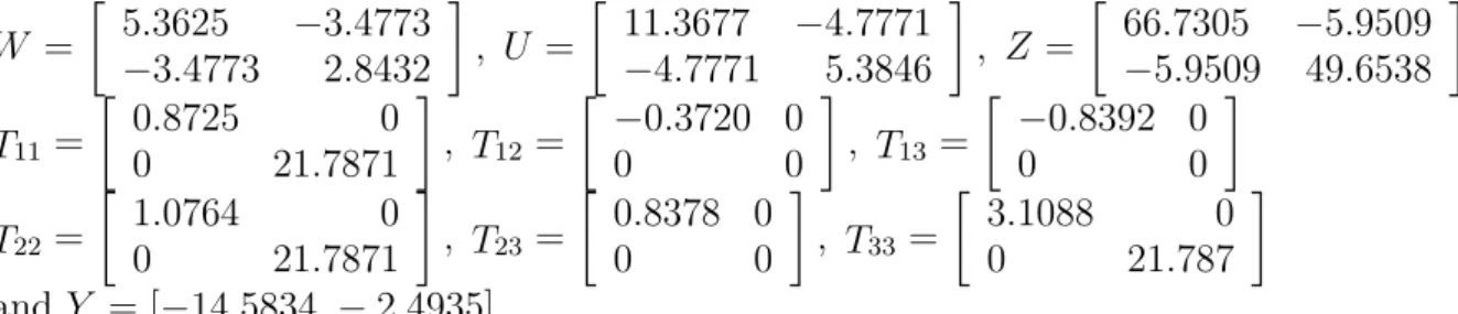
In case of h = 3.6896, solving Theorem 2.1 yields the following set of feasible solutions:

W = [ 5.3625 −3.4773 −3.4773 2.8432 ] , U = [ 11.3677 −4.7771 −4.7771 5.3846 ] , Z = [ 66.7305 −5.9509 −5.9509 49.6538 ] T11 = [ 0.8725 0 0 21.7871 ] , T12= [ −0.3720 0 0 0 ] , T13 = [ −0.8392 0 0 0 ] T22 = [ 1.0764 0 0 21.7871 ] , T23= [ 0.8378 0 0 0 ] , T33 = [ 3.1088 0 0 21.787 ] and Y = [−14.5834 − 2.4935] .

Figures 1 and 2 show that the unstable plant is stabilized by the feedback control. Figure 1 shows the open-loop response, and it can be clearly seen that, in the absence of any control, the system is unstable. Figure 2 shows the closed-loop system response and clearly demonstrates that, under the influence of the proposed controller (5), the system (30) is asymptotically stable for h≤ 3.68.

Example 4.2. Consider the following singular uncertain system with time-varying delay

in the state

where E =   11 −1 11 0 2 0 1  , A0 =   1.5 0.5 1_{−1 0 1} 0.5 0 1  , A1 =   −1 0 −11 −1 0.5 0.3 0.5 −1  , B =   1 11 0 0 1  

and ∆A0(t), ∆A1(t) and ∆B(t) are of the form of (3) with M =

  0.50.2 0.1  , N0 = [ 0.2 0.1 0.3 ], N1 = [ 0.1 0.2 0.5 ], Nb = [ 0.1 0.1 ].

Figure 1. Open-loop system response

Solution: By taking the parameters hd = 0 with these sets of data, for h = 9.6896, using Matlab LMI Control Toolbox to solve the LMIs (17a)-(17c), we obtain the feasible solution: W =   0.61150.1524 0.15241.3686 −0.62310.5709 0.5709 −0.6231 0.9910   , U =   3.03702.0391 2.03914.6329 −1.13871.6670 1.6670 −1.1387 2.6294   , Z =   48.388414.0950 14.095057.6352 −9.24508.6580 8.6580 −9.2450 45.5836   , T11=   7.25467.2147 7.21477.2420 −7.2147−7.2273 −7.2147 −7.2273 7.2420   , T12=   −0.0116 0.0024 −0.0092_{−0.0072 0.0049 −0.0024} −0.0188 0.0073 −0.0115   , T13=   −0.0882 0.0262 −0.06300.0265 −0.0320 −0.0071 −0.0618 −0.0057 −0.0701   , T22=   7.28757.1900 7.19007.2530 −7.2000−7.2347 −7.2000 −7.2347 7.2429   , T23=   _{−0.0264 0.0319 0.0071}0.0881 −0.0262 0.0629 0.0618 0.0057 0.0701   , T33=   8.00446.8931 6.89317.4570 −6.5505−7.0922 −6.5505 −7.0922 7.8407   , ε = 4.0097, Y = [ −2.8092 −4.2875 1.3681 −2.7746 1.9751 −4.4659 ]

and the stabilizing memoryless state feedback control law can be obtained as

u(t) = [ −120.3095 59.4744 108.0832 15.6177 −9.0289 −19.1805 ] x(t).

Hence, according to Theorem 2.2, controller (5) with gain K given in the preceding text stabilizes system (31).

Example 4.3. Consider the uncertain unforced part of system (1) with E = [ 1 0 0 0 ] , A0 = [ −0.9 0 0.5 −2 ] , A1 = [ −1 0 −1 −0.9 ]

, and ∆A0(t) and ∆A1(t) are of the form of (3)

with M = [ 0.5 0.5 ] , N0 = [ 1 1 ], N1 = [ 0.5 0.5 ].

Solution: Table 1 provides the comparison of maximum allowable delay bound (MADB)

h for various hd by different methods. It is easy to get that, for this example, the delay-dependent stability condition in this paper gives better results than those in [15,17].

Furthermore, by taking the decay rateα, and from Corollary 3.1, we obtain the max-imum allowable delay bound (MADB) h as shown in Table 2 below. Note that as α increases, the maximum allowable h decreases.

Example 4.4. Consider the following uncertain singular time delay system

E ˙x(t) = (A0+ ∆A0(t))x(t) + (A1+ ∆A1(t))x(t− h(t)) (32) where E = [ 2 0 0 0 ] , A0 = [ 1 0 0 −2 ] , A1 = [ −2.4 2 0 1 ]

, the uncertain matrices ∆A0(t)

and ∆A1(t) are of the form of (3) with M = λI, Na = Nb = 0.5I. Now, our problem is

to estimate the maximum allowable delay bound (MADB) h to keep the stability of system (32).

Table 1. Comparison of delay-dependent result of Example 4.3 XXXXX XXXXX_XX Methods hd 0.2 0.3 0.4 0.5 0.6

Yue and Han [17] 1.5836 1.4897 1.3942 1.2946 1.1843 Wu et al. [15] 1.5895 1.5007 1.4131 1.3251 1.2315 Corollary 3.1 4.9809 4.6067 4.2453 3.8901 3.5244

Table 2. Maximum allowable delay bound (MADB) h for various stability degree α with hd= 0.5

α 0.1 0.3 0.5 0.7 0.9

Corollary 3.1 2.3391 1.9990 1.5456 1.2345 0.9959

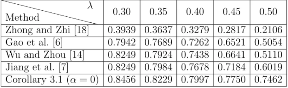
Table 3. Comparison of delay-dependent stability condition of Example 4.4

XXXXX

XXXXX_XX

Method

λ

0.30 0.35 0.40 0.45 0.50

Zhong and Zhi [18] 0.3939 0.3637 0.3279 0.2817 0.2106 Gao et al. [6] 0.7942 0.7689 0.7262 0.6521 0.5054 Wu and Zhou [14] 0.8249 0.7924 0.7438 0.6641 0.5110 Jiang et al. [7] 0.8249 0.7984 0.7678 0.7184 0.6019 Corollary 3.1 (α = 0) 0.8456 0.8229 0.7997 0.7750 0.7462

Solution: Fixing hd = 0 and λ = 0.1, by using the LMI Toolbox in MATLAB (with accuracy 0.01), this above uncertain singular time delay system (32) is asymptotically stable for delay time satisfying h≤ 0.9387. The maximum allowable delay bound (MADB)

h form Corollary 3.1 is shown in Table 3. For comparison, the table also lists the upper

bounds obtained from the criteria in [6,7,14,18]. It can be seen that our methods are less conservative.

5. Conclusion. This paper discusses the problems of the delay-dependent robust sta-bility and stabilization of singular uncertain systems with time-varying delays. Delay-dependent stability criteria are derived by taking the relationships between the terms in the Leibniz-Newton formula into account. Integral inequality approach (IIA) is employed to express these relationships, and they are easy to obtain because the new criteria are based on linear matrix inequalities (LMIs). Moreover, the stability criteria are extended to the design of a stabilizing state feedback controller. Numerical examples demonstrate that these criteria are effective and are an improvement on previous ones.

REFERENCES

[1] E. K. Boukas and Z. K. Liu, Deterministic and Stochastic Time Delay Systems, Springer-Verlag, New York, 2002.

[2] E. K. Boukas and Z. K. Liu, Delay-dependent stability analysis of singular linear continuous-time system, IEE Proc. of Control Theory & Applications, vol.150, pp.325-330, 2003.

[3] E.-K. Boukas and N. F. Al-Muthairi, Delay-dependent stabilization of singular linear systems with delays, International Journal of Innovative Computing, Information and Control, vol.2, no.2, pp.283-291, 2006.

[4] S. Boyd, L. E. Ghaoui, E. Feron and V. Balakrishnan, Linear Matrix Inequalities in System and Control Theory, SIAM, Philadelphia, PA, 1994.

[6] H. Gao, S. Zhu, Z. Cheng and B. Xu, Delay-dependent state feedback guaranteed cost control uncertain singular time delay systems, Proc. of IEEE Conference on Decision and Control, and European Control Conference, pp.4354-4359, 2005.

[7] Z. H. Jiang, W. H. Gui and Y. F. Xie, A less conservative delay-dependent stability for uncertain singular linear systems with time-delays, Proc. of the 8th World Congress on Intelligent Control and Automation, Jinan, China, pp.3673-3678, 2010.

[8] F. L. Lewis, A survey of linear singular systems, Circuits Systems Signal Processing, vol.5, pp.3-36, 1986.

[9] P. L. Liu, Exponential stability for linear time-delay systems with delay dependence, Journal of the Franklin Institute, vol.340, pp.481-488, 2003.

[10] P. L. Liu, Robust exponential stability for uncertain time-varying delay systems with delay depen-dence, Journal of Franklin Institute, vol.346, pp.958-968, 2009.

[11] P. L. Liu, Further results on the exponential stability for time-delay systems with delay dependence, International Journal of Electrical Engineering, vol.17, pp.155-160, 2010.

[12] Y. J. Sun, Exponential stability for continuous-time singular systems with multiple time delays, Journal of Dynamic Systems Measurement and Control, vol.125, no.2, pp.262-264, 2003.

[13] X. Sun and Q. Zhang, Delay-dependent robust stabilization for a class of uncertain singular de-lay systems, International Journal of Innovative Computing, Information and Control, vol.5, no.5, pp.1231-1242, 2009.

[14] Z. G. Wu and W. N. Zhou, Delay-dependent robust stabilization for uncertain singular systems with state delay, Acta Automatica Sinica, vol.33, pp.714-718, 2007.

[15] Z. G. Wu, H. Y. Su and J. Chu, Robust exponential stability of uncertain singular Markovian jump time-delay systems, Acta Automatica Sinica, vol.36, pp.58-563, 2010.

[16] D. Yue, J. Lam and D. W. C. Ho, Delay-dependent robust exponential stability of uncertain descrip-tor systems with time-varying delays, Dynamics of Continuous, Discrete and Impulsive Systems, Series B, vol.12, no.1, pp.129-149, 2005.

[17] D. Yue and Q. H. Han, Delay-dependent robust H∞ controller design for uncertain descriptor

sys-tems with time-varying delays discrete and distributed delays, IEE Proc. of Control Theory and Applications, vol.152, pp.628-638, 2005.

[18] R. X. Zhong and Y. Zhi, Delay-dependent robust control of descriptor systems with time delay, Asian Journal of Control, vol.8, pp.36-44, 2006.