Generalized projective synchronization of chaotic systems
with unknown dead-zone input: Observer-based approach
Yung-Ching Hung, Chi-Chuan Hwang, and Teh-Lu Liaoa兲
Department of Engineering Science, National Cheng Kung University, Tainan, 701 Taiwan Jun-Juh Yan
Department of Computer and Communication, Shu-Te University, Kaohsiung 824, Taiwan 共Received 11 April 2006; accepted 21 July 2006; published online 13 September 2006兲
In this paper we investigate the synchronization problem of drive-response chaotic systems with a scalar coupling signal. By using the scalar transmitted signal from the drive chaotic system, an observer-based response chaotic system with dead-zone nonlinear input is designed. An output feedback control technique is derived to achieve generalized projective synchronization between the drive system and the response system. Furthermore, an adaptive control law is established that guarantees generalized projective synchronization without the knowledge of system nonlinearity, and/or system parameters as well as that of parameters in dead-zone input nonlinearity. Two illus-trative examples are given to demonstrate the effectiveness of the proposed synchronization scheme. © 2006 American Institute of Physics.关DOI:10.1063/1.2336728兴
Generally, chaotic systems are nonlinear deterministic systems that possess complex and unpredictable behavior. Chaos control and chaos synchronization as well as its applications have been developed and thoroughly studied over the past two decades. The typical configuration of the synchronization of chaotic systems consists of drive and response systems. The drive system drives the re-sponse system via coupling signal(s) to synchronize each other’s behavior. There are several different types of syn-chronizations have been proposed in the literature such as complete synchronization (CS), phase synchronization (PS), lag synchronization (LS), generalized synchroniza-tion (GS), and generalized projective synchronizasynchroniza-tion (GPS). In the past decade, based on the state observer design technique, many observer-based synchronization schemes have been proposed. However, in practice, the values of parameters and nonlinearities that exist in cha-otic systems and in the control input are partially known
a priori. These parametric uncertainties and
nonlineari-ties will destroy the synchronization performance. In this paper we demonstrate the projective synchronization of chaotic systems without the knowledge of these paramet-ric uncertainties and nonlinearities via a state observer technique and adaptive control scheme.
I. INTRODUCTION
The synchronization of chaotic systems has received great attention over past few years. Several theoretical stud-ies and/or laboratory experimentations have demonstrated
the pivotal role of this phenomenon in secure
communications.1–9 The preliminary configuration of chaos synchronization consists of two chaotic systems: a drive sys-tem and a designed response syssys-tem. The drive syssys-tem drives
the response system via the transmitted signal共s兲 so that the trajectory of drive system synchronizes that of the response system. Several different types of synchronizations have been proposed in the literature, for example, complete syn-chronization 共CS兲,10–13 phase synchronization 共PS兲,14,15 lag synchronization 共LS兲,16,17 generalized synchronization 共GS兲,18–23
as well as generalized projective synchronization 共GPS兲,24–36
Complete synchronization, which implies states of the drive and response systems, are synchronized. The phase synchronization occurs in a manner that phases are locked together, but the amplitude may evolve incoherently. Lag synchronization that appears as a coincidence of state of the drive system at lagged time and that of response system at current time. The generalized synchronization means that states of the response system synchronize that of the drive system through a nonlinear smooth functional mapping. Generalized synchronization has been demonstrated by non-identical chaotic systems and in distinct classes of chaotic systems. Generalized projective synchronization, which be-longs to a subclass of the generalized synchronization, uni-fies different types of synchronization phenomena such as antiphase synchronization and complete synchronization, as well as a specific case of generalized synchronization into one by a scaling factor. The performance of projective syn-chronization can be selected and manipulated by controlling the scaling factor.24–36
However, from the viewpoint of control theory, the re-sponse system can be considered an observer of the drive system. All the state variables of the response system are constructed by a transmitted signal from the drive system, and then, all or partial state trajectories of these systems are driven into synchronization through an appropriate control design for the observer. Based on the observer design tech-nique, many observer-based synchronization schemes have been proposed.30,32,37The control schemes with state feed-back or output feedfeed-back for chaos synchronization can be a兲Corresponding author. Telephone:⫹886-6-2757575 #63337.
Fax:⫹886-6-2766549. Electronic mail: [email protected]
realized by electronic components such as operational ampli-fier共OPA兲, resistor, and capacitor, etc. or by electromechani-cal actuators. However, in practice, there always exist non-linearities, including the saturation, backlash, and dead zone in OPA-based circuits or electromechanical devices. Further-more, it is difficult to maintain the exact values of resistance and capacitance due to the uncontrollable environmental conditions and to know the exact parameters共e.g., width and slope兲 of the dead zone. These input nonlinearities and para-metric uncertainties may lead to serious degradation of sys-tem performance and cause syssys-tem instability. Therefore, it is clear that the effects of input nonlinearities with unknown parameters must be taken into account when analyzing and implementing the synchronization control scheme.
Motivated by the aforementioned results, an observer-based response system with a dead zone in control input is designed to ensure the synchronization between the drive and response systems coupled with a scalar transmitted sig-nal. Both nonadaptive and adaptive output feedback control techniques are employed to obtain the generalized projective synchronization of drive-response chaotic systems. Two well-known Chua’s system and Van der Pol-Duffing oscilla-tor are given as illustrative examples to demonstrate the ef-fectiveness of the proposed projective synchronization scheme.
Notation: Note that throughout the remainder of this paper, the notation MT denotes the transpose of a square matrix M, while for x苸Rn,储x储 =共xTx兲1/2denotes the
Euclid-ean norm of the vector; P⬎0 denotes P is a symmetric posi-tive definite symmetric matrix and P = PT⬍0 denotes P is a symmetric negative definite symmetric matrix. min共P兲 de-notes the smallest eigenvalue of the matrix P.
II. PROBLEM FORMULATION
Generally, dynamics of many chaotic systems can be de-composed into below two parts: a linear dynamics with re-spect to state and a nonlinear feedback part with rere-spect to the system output. Therefore, a class of chaotic systems is considered here and its dynamics are described by the fol-lowing form:
x˙ = Ax + f共y兲 + B关Tg共x,y兲兴, y = CTx, 共1兲
where 共·兲T denotes the vector transpose; y苸R denotes the system output; x苸Rn represents the state vector, and A, B, and C denote known system matrices with appropriate di-mensions. The pair 共A,B兲 is controllable, i.e., the controlla-bility matrix关B,AB, ... ,An−1B兴 is in full rank, and, further-more, the pair 共CT, A兲 is observable, namely, the observability matrix 关C,ATC , . . . ,共AT兲n−1C兴T is in full rank. Assuming that 苸Rp and g苸Rp are real analytic vectors with f共0兲=0 and g共0,0兲=0, respectively. Furthermore, we assume that the system共1兲 has a unique solution x共t兲 passing through the initial state x共0兲=x0 and this solution is well defined over an interval 关0 ⬁兲.
For the class of systems 共1兲, we make the following assumption.
共A1兲 For the nonlinear function T
g共x,y兲 in 共1兲, there
exist constants 0⬍i
*⬍⬁, i=1, ... ,p and the nonlinear
func-tions g¯i共y兲, i=1, ... ,p, such that 兩T
g共x,y兲兩 ⱕ
兺
i=1 pi*兩g¯i共y兲兩, for all x 苸 Rnand y苸 R. 共2兲 Owing to the matrix A is generally unstable and共CT, A兲 is observable, a constant vector L苸Rn can be chosen such that共A−LCT兲 is stable and a strictly positive real system can be obtained. Hence, to ensure the stability of the overall drive-response chaos synchronization, the following assump-tion is made:
共A2兲 There is a constant vector L苸Rn
such that the transfer function H共s兲=CT关sI−共A−LCT兲兴−1B is strictly
posi-tive real.
According to the Kalman and Yakubovich Lemma共K-Y lemma兲,38the strict positive realness of H共s兲 guarantees that
for a given matrix Q = QT⬎0, there exists a matrix P= PT ⬎0 such that the following conditions:
共A − LCT兲T
P + P共A − LCT兲 = − Q, PB = C, 共3兲
hold.
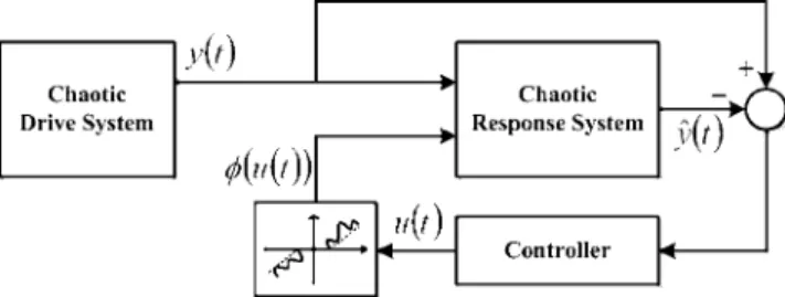
Our objective in this study is stated as follows: given the drive system as共1兲, an observer-based response system with dead-zone nonlinearity in control input will be designed and be driven by a scalar available transmitted signal so that states of the response system will synchronize that of the system共1兲 through a scaling factor. The overall synchroniza-tion system is schematically depicted in Fig. 1.
III. OBSERVER-BASED CHAOS SYNCHRONIZATION SCHEMES
On the basis of state observer design, a response system in the driver-response configuration of chaos synchronization corresponding to 共1兲 is given as follows:
xˆ˙ = Axˆ +f共y兲 + L共y − yˆ兲 − B共u兲, yˆ = CTxˆ, 共4兲
where xˆ denotes the state of the response system and the constants vector L苸Rn is chosen such that共A−LCT兲 is an exponentially stable matrix. Here u is the control input that will be appropriately designed to obtain the generalized pro-jective synchronization between 共1兲 and 共4兲 subject to the system’s nonlinearities and/or unknown parameters.
With the coupled systems 共1兲 and 共4兲, the generalized projective synchronization can be characterized by synchro-nizing x and xˆ asymptotically, i.e., limt→⬁储x−xˆ储 =0, where is called the “scaling factor.” Moreover, to
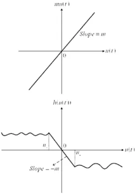
ment the practical control input in共4兲, the dead-zone nonlin-ear function 共u兲, as shown in Fig. 1, is imposed on the control input u. The dead-zone nonlinear function 共u兲 can be decomposed into two parts that is defined as follows:
关u共t兲兴 = mu共t兲 + h关u共t兲兴, 共5兲
where m⬎0 is called the general slope of the dead zone and the nonlinear function h关u共t兲兴 is given as follows:
h关u共t兲兴 =
冦
− mu++1关u共t兲兴, u共t兲 ⱖ u+,
− mu共t兲, u−⬍ u共t兲 ⬍ u+,
− mu−+2关u共t兲兴, u共t兲 ⱕ u−,
共6兲 where 0ⱕu+⬍⬁ and −⬁ ⬍u−ⱕ0 are two constants speci-fying the size of the dead zone. Furthermore, the nonlinear functions 1关u共t兲兴 and2关u共t兲兴 satisfy 0ⱕ1关u共t兲兴ⱕ1共max兲 and −2共max兲ⱕ2关u共t兲兴ⱕ0, respectively, for all u共t兲苸R. The
decomposition of共u兲 is schematically depicted in Fig. 2. On the basis of the property of nonlinear function h关u共t兲兴 as given in共6兲, it is obvious that h关u共t兲兴 is always bounded, i.e., there exist a positive constant*large enough such that
兩h关u共t兲兴兩 ⱕ max兵兩mu+兩,兩− mu−兩,兩− mu++1共max兲兩,兩− mu−
−2共max兲兩其 ⱕ*⬍ ⬁ . 共7兲
To aim the projective synchronization, let us define the state error e =x−xˆ and the output error e1=y−yˆ; the error
dy-namics from 共1兲 and 共4兲 with 共5兲 can be expressed by
e˙ =x˙ − xˆ˙ = 共A − LCT兲e + B兵关Tg共x,y兲兴 + mu + h共u兲其,
共8兲
e1= CTe.
A. Nonadaptive control scheme
If all constantsi*, i = 1 , . . . , p, and* in共2兲 and 共7兲 are well known, the control input for the generalized projective synchronization is derived as follows:
u = −
冋
兩兩冉
兺
i=1 p i* m兩g¯i共y兲兩冊
+ * m册
sign共e1兲. 共9兲Consider the stability of the error dynamical system共8兲 un-der the control law 共9兲; we choose a Lyapunov function as
V共t兲 = 1 me
T共t兲Pe共t兲, 共10兲
where P = PT⬎0 satisfies Eq. 共3兲. It is obvious that V is a positive and decrescent function. Furthermore, V is radically unbounded.
Taking the time derivative of V along the trajectories of the resulting error dynamical system共8兲 with 共9兲 and apply-ing the K-Y lemma 共3兲 and property of nonlinear function
h关u共t兲兴 共7兲 yields V˙ = 1 m兵e T关共A − LCT兲T P + P共A − LCT兲兴e其 + 2 m„e T PB兵关Tg共x,y兲兴 + mu + h共u兲其… = − 1 m共e T Qe兲 + 2 m„C T e兵关Tg共x,y兲兴 + mu + h共u兲其… ⱕ − 1 m共e T Qe兲 + 2 m兩储e1兩
冉
兺
i=1 p i *兩g¯ i共y兲兩冊
+ 2e1u + 2 m兩e1兩 * = − 1 m共e TQe兲 ⱕ 0. 共11兲From共11兲, we have V˙, which is negative semidefinite, and it follows that the equilibrium points e = 0 of system 共8兲 are uniformly globally stable, i.e., e共t兲苸L⬁ 关e共t兲 is a bounded
signal for all tⱖ0兴. Moreover, from 共8兲 and 共11兲, we can easily show that e˙共t兲苸L⬁and e共t兲苸L2关the square of e共t兲 is
integrable with respect to time兴. Therefore, by Barbalat’s lemma,39 we conclude that e共t兲→0 as t→⬁, which means that for the drive chaotic system共1兲 satisfying the 共A1兲 and 共A2兲 and the observer-based response system 共4兲 with the dead zone in input, the proposed control law共9兲 will achieve the generalized projective synchronization asymptotically, i.e., 储e共t兲储 =储x共t兲−xˆ共t兲储 →0 as t→⬁ for all initial condi-tions. Furthermore, all signals inside the closed-loop system remain bounded.
B. Adaptive control scheme
The control law derived thus far requires that the knowl-edge of the system’s parameters i
*
, i = 1 , . . . , p, and param-eter *of the dead-zone model. However, in many real ap-plications it is difficult to exactly determine both the values of the system’s parameters i
*
, i = 1 , . . . , p, and parameter* of the dead-zone nonlinearity. Consequently, the control law
u given in共9兲 cannot be easily obtained to ensure the
gener-alized projective synchronization. To overcome these
backs, let us redefine the control parameters in 共9兲 as fol-lows: i=i
*/ m and =*/ m, and an adaptive control law
withˆi, i = 1 , . . . , p, andˆ , whereˆiandˆ are estimates ofi and , is designed to derive the adaptive response system, and thereby achieving the generalized projective synchroni-zation between the drive system and the response system. Now, similar to 共9兲, the adaptive control law with the esti-mates of ˆi, i = 1 , . . . , p, andˆ is derived as follows:
u = −
冋
兩兩冉
兺
i=1 pˆ
i兩g¯i共y兲兩
冊
+ˆ册
sign共e1兲. 共12兲The estimatesˆi, i = 1 , . . . , p, andˆ are updated according to the following algorithm:
ˆ˙i=兩兩兩e
1兩兩g¯i共y兲兩, withˆi共0兲 ⱖ 0, i = 1, ... ,p, 共13兲
ˆ˙ =␥1兩e1兩, withˆ共0兲 ⱖ 0, 共14兲
where␥1is a positive constant specified by the designer. The
proposed adaptive control scheme will guarantee the globally asymptotic stability of the error system 共8兲 and achieve the synchronization objective.
Let us first define the following parameter errors: i =i−ˆi, i = 1 , . . . , p,and =−ˆ ;then consider a Lyapunov function as follows: V共t兲 = 1 me T共t兲Pe共t兲 +
兺
i=1 p i 2共t兲 + 1 ␥1 2共t兲. 共15兲It is obvious that V is a positive and decrescent function. Furthermore, V is radically unbounded.
Taking the time derivative of V along the trajectories of the resulting error dynamical system共8兲 with 共9兲 and apply-ing共3兲 and 共7兲 leads to
V˙ = 1 me T关共A − LCT兲T P + P共A − LCT兲兴e + 2 me T PB兵关Tg共x,y兲兴共u兲其 + 2
兺
i=1 p i˙i+ 2 ␥1 ˙ = − 1 m共e TQe兲 + 2 me1兵关 Tg共x,y兲兴 + mu + h共u兲其 + 2兺
i=1 p i˙i+ 2 ␥1 ˙ . 共16兲Since i is constant, ˙i= 0 and the following expression holds:
˙
i= −ˆ˙i, i = 1, . . . , p, 共17兲 andis constant,˙ = 0, and the following expression holds:
˙ = −ˆ˙ 共18兲
Substituting 共13兲, 共14兲, 共17兲, and 共18兲 into 共16兲, we can get the following result:
V˙ = − 1 m共e TQe兲 + 2 me1兵关 Tg共x,y兲兴 + mu + h共u兲其 + 2
兺
i=1 p i˙i+ 2 ␥1 ˙ ⱕ − 1 m共e TQe兲 + 2 m兩e1兩兩兩兩 Tg共x,y兲兩 + 2e 1u + 2 m兩e1兩 ⫻兩h共u兲兩 − 2兺
i=1 p iˆ˙i− 2 ␥1 ˆ˙ ⱕ − 1 m共e T Qe兲 + 2兩e1兩兩兩冉
兺
i=1 p i * m兩g¯i共y兲兩冊
+ 2e1u + 2 * m兩e1兩 − 2兺
i=1 p iˆ˙i− 2 ␥1 ˆ˙ = − 1 m共e T Qe兲 + 2兩e1兩兩兩冉
兺
i=1 p i兩g¯i共y兲兩冊
+ 2e1u + 2兩e1兩 − 2兺
i=1 p iˆ˙i− 2 ␥1 ˆ˙ = − 1 m共e T Qe兲 + 2兩e1兩兩兩冉
兺
i=1 p 共i+ˆi兲兩g¯i共y兲兩冊
+ 2e1u + 2共+ˆ兲兩e1兩 − 2兺
i=1 p i关兩e1兩兩兩兩g¯i共y兲兩兴 − 2 ␥1 共␥1兩e1兩兲 = − 1 m共e T Qe兲 + 2兩e1兩兩兩兺
i=1 p ˆ i兩g¯i共y兲兩 + 2e1u + 2ˆ兩e1兩 = − 1 m共e T Qe兲 ⱕ 0. 共19兲From共19兲, we have V˙, which is negative semidefinite, and it follows that the overall systems are uniformly stable, i.e.,
e共t兲苸L⬁, 共t兲苸L⬁, and 共t兲苸L⬁, as well as u共t兲苸L⬁. Moreover, from 共8兲 and 共19兲, we can easily show that e˙共t兲 苸L⬁ and e共t兲苸L2. Therefore, from Barbalat’s lemma, we
conclude that e共t兲→0 as t→⬁, which means that for the drive chaotic system共1兲 satisfying the 共A1兲 and 共A2兲 and the observer-based response system 共4兲 with the dead zone in control input, the proposed adaptive control law 共12兲 with adaptation laws 共13兲 and 共14兲 will achieve the generalized projective synchronization asymptotically, i.e., 储e共t兲储 =储x共t兲−xˆ共t兲储 →0 as t→⬁ for all initial conditions. Further-more, all signals inside the closed-loop system remain bounded.
IV. ILLUSTRATIVE EXAMPLES
To illustrate the effectiveness of the proposed adaptive synchronization scheme, two examples of well-known cha-otic systems: Chua’s system and Van der Pol-Duffing oscil-lator are considered and their numerical simulations are per-formed.
Example 1 Chua’s system:
A nondimensional differential equation for Chua’s sys-tem is given by x˙1=␣关x2− x1− f共x1兲兴, x˙2= x1− x2+ x3, 共20兲 x˙3= −1x2−2x3, and f共x1兲 = bx1+ 0.5共a − b兲共兩x1+ 1兩 − 兩x1+ 1兩兲, 共21兲
where␣,1, and2are system parameters and are given as
follows: ␣= 10, 1= 15, and 2= 0.0385; f共x1兲 denotes a
three-segment piecewise linear function in which a , b are two negative real constants and a⬍−1, −1⬍b⬍0. Herein, the parameters aand b are assumed to be unknown. By
in-troducing y = x1, Eq.共20兲 can be rewritten in a compact form as follows: x˙ =
冤
− 10 10 0 1 − 1 1 0 − 15 − 0.0385冥
x +冤
1 0 0冥
关− 10by − 5共a − b兲共兩y + 1兩 − 兩y + 1兩兲兴 ⬅ Ax + B关T
g共y兲兴, 共22兲
y = x1=
关
1 0 0兴
x⬅ CTx, 共23兲where T=关
1 2兴=关−10b −5共a−b兲 兴 and g共y兲
=关g1共y兲 g2共y兲 兴=关y 兩y+1兩−兩y+1兩 兴. It can be easily verified
that共A,B兲 is a controllable pair and 共CT, A兲 is an observable pair. Also, the vector LT=关−7 1.9536 0.7343 兴 can be
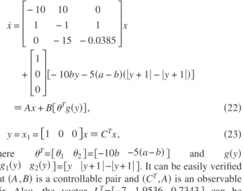
FIG. 3.共a兲 Trajectories of state error between the drive and response system when =1. 共b兲 Trajectories of state error between the drive and response system when =−1.
found so that the eigenvalues of matrix 共A−LCT兲 are −2.3532 and −1.0159± j4.8231, and that the transfer func-tion H共s兲=CT关sI−共A−LCT兲兴−1B =共s2+ 1.385s + 15.38兲/共s3
+ 4.385s2+ 29.085s + 57.17兲 is strictly positive real. Hence, 共A1兲 and 共A2兲 are satisfied. Moreover, the symmetric and positive definite matrices P and Q satisfying Eq.共3兲 are
P =
冤
1 0 0 0 11 − 0.6667 0 − 0.6667 0.8658冥
, 共24兲 Q =冤
6 0.0001 0 0.0001 2 1.0637 0 1.0637 2冥
.As derived earlier, an observer-based response system is de-signed as follows: xˆ˙ =
冤
− 10 10 0 1 − 1 1 0 − 15 − 0.0385冥
xˆ + L共y − yˆ兲 −冤
1 0 0冥
共u兲, 共25兲 yˆ =关
1 0 0兴
xˆ,and the adaptive control law is designed as follows:
u = −兵兩兩关ˆ1兩y兩 +ˆ2共兩y + 1兩 − 兩y + 1兩兲兴 +ˆ其sign共e1兲, 共26兲
where the estimate ˆ1 and ˆ2 are updated according to
fol-lowing algorithm: ˆ˙
1=兩兩兩e1兩兩y兩,
共27兲 ˆ˙
2=兩兩兩e1兩兩兩y + 1兩 − 兩y + 1兩兩, ˆ˙ =兩e1兩,
and the nonlinear input containing a dead zone is defined as
FIG. 4. 共a兲 Trajectories of estimated parameters when =1. 共b兲 Trajectories of estimated parameters when = −1.
关u共t兲兴 =
冦
共u共t兲 − u+兲兵1 − 0.3 sin关u共t兲兴其, u共t兲 ⬎ u+,
0, u−ⱕ u共t兲 ⱕ u+,
共u共t兲 − u−兲兵1 − 0.3 cos关u共t兲兴其, u共t兲 ⬍ − u−.
共28兲 As given in 共5兲 and 共6兲, we can obtain m=0.7, 1关u共t兲兴
= 0.3u+sin关u共t兲兴 and 2关u共t兲兴=0.3u−cos关u共t兲兴. In numerical
simulations, the system’s parameters are chosen as a = −1.28, b = −0.69, thereby implying 1= 6.9 and 2= 2.95.
The parameters in the dead zone are chosen as follows: u+
= 5 and u−= −3. Figures 3共a兲 and 3共b兲 show the error
trajec-tories of the generalized projective synchronization for Chua’s circuits with the scaling factors =1 and =−1, re-spectively. The initial values of the update law is given as ˆ
1共0兲=0,ˆ2共0兲=0, andˆ共0兲=0. The initial states of the drive
and response system are given as 关xd1共0兲xd2共0兲xd3共0兲兴 =关0.1−0.10.1兴, 关xr1共0兲xr2共0兲xr3共0兲兴=关6−32兴, respectively. Figures 4共a兲 and 4共b兲 show trajectories of the estimated
pa-rameters when =1 共complete synchronization兲 and =−1 共antiphase synchronization兲, respectively.
Example 2 Van der Pol-Duffing oscillator:
In this example, we consider the chaotic synchronization of two unidirectionally coupled Van-der-Pol-Duffing oscillators.40–42The drive generators described by system of dimensionless differential equations:
x˙1= −v共x1 3
−␣x1− x2兲, x˙2= x1− x2− x3, x˙3=x2,
共29兲 where ␣, , and v are three positive real parameters. The
system exhibits bistable chaotic dynamics if the parameters are set equal to␣= 0.35,= 300, andv = 100.
Herein, the parameters␣andv are perturbed by⌬␣and ⌬v, respectively. By introducing y=x1, Eq. 共29兲 can be
re-written in a compact form as follows:
FIG. 5.共a兲 Trajectories of state error between the drive and response system when =1. 共b兲 Trajectories of state error between the drive and response system when =−1.
x˙ =
冤
35 100 0 1 − 1 − 1 0 300 0冥
x +冤
− 100y3 0 0冥
+冤
1 0 0冥
⫻关⌬vy3+共100⌬␣+ 0.35⌬v + ⌬␣⌬v兲y + ⌬vx 2兴 ⬅ Ax + f共y兲 + B关T g共x,y兲兴, 共30兲 y = x1=关
1 0 0兴
x⬅ CTx, 共31兲where the parameter defined as T=关1 2 3兴
=关⌬v 共100⌬␣+ 0.35⌬v+⌬␣⌬v兲 ⌬v 兴 and g共x,y兲T
=关g1共x,y兲 g2共x,y兲 g3共x,y兲 兴=关y3 y x2兴. It can be easily
verified that 共A,B兲 is a controllable pair and 共CT, A兲
is an observable pair. Also, the vector LT
=关36 1.3333 −0.3311 兴 can be found so that the eigenval-ues of matrix共A−LCT兲 are −0.9993 and −0.5003± j18.2505, and that the transfer function H共s兲=CT关sI−共A−LCT兲兴−1B
=共s2+ s + 300兲/共s3+ 2s2+ 334.3s + 333.1兲 is strictly positive real. Hence,共A1兲 and 共A2兲 are satisfied. Moreover, the sym-metric and positive definite matrices P and Q satisfying Eq. 共3兲 are
FIG. 6. 共a兲 Trajectories of estimated parameters when =1. 共b兲 Trajectories of estimated parameters when = −1.
P =
冤
1 0 0 0 301 1 0 1 1.0067冥
, 共32兲 Q =冤
2 − 0.0078 0 − 0.0078 2 − 0.01 0 − 0.01 2冥
.As derived earlier, an observer-based drive system is de-signed as follows: xˆ˙ =
冤
35 100 0 1 − 1 − 1 0 300 0冥
xˆ +冤
− 100y3 0 0冥
+ L共y − yˆ兲 −冤
1 0 0冥
共u兲, 共33兲 yˆ =关
1 0 0兴
xˆ,and the control law is designed as follows:
u = −关兩兩共ˆ1兩y3兩 +ˆ2兩y兩 +ˆ3兲 +ˆ兴sign共e1兲, 共34兲
where the estimate ˆ1,ˆ2, and ˆ3 are updated according to
the following algorithm: ˆ˙
1=兩兩兩e1兩兩y3兩, ˆ˙2=兩兩兩e1兩兩y兩,
共35兲 ˆ˙
3=兩兩兩e1兩, ˆ˙ =兩e1兩,
and the nonlinear input containing a dead zone is defined as 关u共t兲兴 =
冦
共u共t兲 − u+兲兵1 − 0.3 sin关u共t兲兴其, u共t兲 ⬎ u+,
0, u−ⱕ u共t兲 ⱕ u+,
共u共t兲 − u−兲兵1 − 0.3 cos关u共t兲兴其, u共t兲 ⬍ − u−.
共36兲 As given in 共5兲 and 共6兲, we can obtain m=0.7, 1关u共t兲兴
= 0.3u+sin关u共t兲兴 and2关u共t兲兴=0.3u−cos关u共t兲兴. In the
numeri-cal simulations, the parametric perturbations⌬␣ and⌬v are chosen as ⌬␣= −0.01 and ⌬v=1, respectively, thereby im-plying 1= 1, 2= −0.66, and 3= 1. Figures 5共a兲 and 5共b兲
show the error trajectories of the generalized projective syn-chronization for Van-der-Pol-Duffing oscillators with the scaling factors=1, =−1, respectively. In numerical simu-lations, the parameters are specified as follows: 共i兲 The pa-rameters in the dead-zone model is given as u+= −5 and u−
= 3.共ii兲 The initial value of update law is given asˆ1共0兲=0,
ˆ
2共0兲=0,ˆ3共0兲=0, andˆ共0兲=0. 共iii兲 The initial value of the
drive and response system is given as 关xd1共0兲 xd2共0兲 xd3共0兲兴 =关0.1 −0.1 0.1兴 and 关xr1共0兲 xr2共0兲 xr3共0兲兴=关2 −2 1兴, re-spectively. Figures 6共a兲 and 6共b兲 show the trajectories of es-timated parameters when =1 共complete synchronization兲 and=−1 共antiphase synchronization兲, respectively. V. CONCLUSIONS
In this work, both nonadaptive and adaptive observer-based approaches have been developed to resolve the gener-alized projective synchronization problem for a class of cha-otic systems in the presence of system’s parametric uncertainties and dead-zone nonlinear in control input. Both drive and response systems are coupled through a scalar
transmitted signal. Given certain structural conditions of the drive chaotic system, an observer-based response system and two control schemes are constructed so that those drive sys-tem and response syssys-tem are to be synchronized. Further-more, the knowledge of parameters in the dead zone and that of the system’s parametric uncertainties are not necessary in the adaptive control design. The synchronization and stabil-ity of the overall systems are guaranteed by the Lyapunov stability theory. Numerical simulations of two well-known chaotic systems: Chua’s circuit and Van der Pol-Duffing os-cillator are given to demonstrate the effectiveness of the pro-posed approach.
1L. M. Pecora and T. L. Carroll, Phys. Rev. Lett. 80, 2109共1990兲. 2L. O. Chua, L. Kocarev, K. Eckert, and M. Itho, Int. J. Bifurcation Chaos
Appl. Sci. Eng. 2, 705共1992兲.
3K. M. Cuomo, A. V. Oppenheim, and S. H. Strogate, IEEE Trans. Circuits
Syst., II: Analog Digital Signal Process. 40, 626共1993兲.
4O. Morgul and E. Solak, Phys. Rev. E 54, 4803共1996兲.
5H. Ohmori, Y. Lto, and A. Sano, Proceedings of the 35th Decision and
Control IEEE, 1996, Vol. 3, p. 2968.
6G. Grassi and S. Mascolo, IEEE Trans. Circuits Syst., I: Fundam. Theory
Appl. 44, 1013共1997兲.
7T. L. Liao and S. H. Tsai, Chaos, Solitons Fractals 11, 1387共2000兲. 8B. Andrievsky, Math. Comput. Simul. 58, 285共2002兲.
9M. Feki, Chaos, Solitons Fractals 18, 141共2003兲.
10H. Fujisaka and T. Yamada, Prog. Theor. Phys. 69, 32共1983兲. 11K. M. Cuomo and A. V. Oppenheim, Phys. Rev. Lett. 71, 65共1993兲. 12S. Hayes, C. Grebogi, E. Ott, and A. Mark, Phys. Rev. Lett. 73, 1781
共1994兲.
13T. L. Carroll, J. F. Heagy, and L. M. Pecora, Phys. Rev. E 54, 4676
共1996兲.
14M. Rosenblum, A. Pikovsky, and J. Kurtz, Phys. Rev. Lett. 76, 1804
共1996兲.
15A. Pikovsky, M. G. Rosenblum, G. V. Osipov, and J. Kurtz, Physica D 104, 219共1997兲.
16K. Hassan, Khalil共Macmillan, New York, 1992兲.
17C. Cailian, F. Gang, and G. Xinping, “IEEE Digital Object Identifier
ACC,” 2005, p. 4277.
18N. F. Rulkov, M. M. Sushchik, L. S. Tsimring, and H. D. I. Abarbanel,
Phys. Rev. E 51, 980共1995兲.
19L. Kocarev and U. Parlitz, Phys. Rev. Lett. 76, 1816共1996兲. 20O. Morgul and E. Solak, Phys. Rev. E 54, 4803共1996兲.
21O. Morgul and E. Solak, Int. J. Bifurcation Chaos Appl. Sci. Eng. 7, 1307
共1997兲.
22H. Nijmeijer and I. M. Y. Mareels, IEEE Trans. Circuits Syst., I: Fundam.
Theory Appl. 44, 882共1997兲.
23K. Josic, Phys. Rev. Lett. 80, 3053共1998兲.
24T. Yang and L. O. Chua, Int. J. Bifurcation Chaos Appl. Sci. Eng. 9, 215
共1999兲.
25Z. Li and D. Xu, Phys. Lett. A 282, 175共2001兲. 26D. Xu, Z. Li, and S. R. Bishop, Chaos 11, 439共2000兲. 27D. Xu, W. L. Ong, and Z. Li, Phys. Lett. A 305, 167共2002兲. 28Z. Li and D. Xu, Chaos, Solitons Fractals 22, 477共2004兲.
29D. Xu, C. Y. Chee, and C. Li, Chaos, Solitons Fractals 22, 175共2004兲. 30G. Wen and D. Xu, Phys. Lett. A 333, 420共2004兲.
31X. S. Wang, C. Y. Su, and H. Hong, Automatica 40, 407共2004兲. 32G. Wen and D. Xu, Chaos, Solitons Fractals 26, 71共2005兲. 33J. Yan and C. Li, Chaos, Solitons Fractals 26, 1119共2005兲. 34G. H. Li, Chaos, Solitons Fractals 29, 490共2006兲. 35G. H. Li, Chaos, Solitons Fractals 30, 77共2006兲.
36C. H. Li and J. Yan, Chaos, Solitons Fractals 30, 140共2006兲.
37T. L. Liao and N. S. Huang, IEEE Circuits Syst. Mag. 46, 1144共1999兲. 38M. Vidyasagar, Nonlinear Systems Analysis 共Prentice-Hall, Englewood
Cliffs, NJ, 1993兲.
39V. M. Popov, Hyperstability of Control System共Springer-Verlag, Berlin,
1973兲.
40F. Hilaire, B. Samuel, and D. Jamal, Chaos, Solitons Fractals 26, 215
共2005兲.
41H. B. Fotsin and P. Woafo, Chaos, Solitons Fractals 24, 1363共2005兲. 42J. C. Ji and C. H. Hansen, Chaos, Solitons Fractals 28, 555共2006兲.