Screening procedure for airborne pollutants emitted from a high-tech industrial complex in Taiwan

Title Page Submitted to: Chemosphere in September 2014 Title:

Screening procedure of airborne pollutants emitted from a high-tech industrial complex in Taiwan

Keywords: air toxics, Gaussian plume equations, high-tech industry, screening procedure Authors:

First author, John H.C. Wang, Enviro Nuclear Services, LLC, Nevada, U.S.A Co-first author, Ching-Tsan Tsai, Department of Public Health, China Medical

University, Taichung, Taiwan

Third author, Chow-Feng Chiang, Department of Health Risk Management, China Medical University, Taichung, Taiwan

J.H.C. Wang and C.T. Tsai have equal contribution to this study Corresponding author:

Chow-Feng Chiang, Professor

E-mail address: [email protected] 886-4-2205-3366 ext 6123

Department of Health Risk Management, China Medical University 91 Hsueh-Shih Road, Taichung 404, Taiwan,

Words and equations:

Abstract: 300 Text: 3884 Table 1 Figure: 5

Total equivalent words: 300+3884+6*300 = 5984 (<6000) Equation: 7

Screening procedure of airborne pollutants emitted from a high-tech industrial complex in Taiwan

John H.C. Wang, Ching-Tsan Tsai, Chow-Feng Chiang

Abstract

Even with modern computerized techniques, the atmospheric dispersion modeling has never been an easy task as it requires the inputs of tremendous amount of inter-related data with wide dissimilarity to a study site. The ever increasing air pollutants for

regulation further complicate the difficulty. The challenge prompts this study to develop a simplified screening procedure for long-term exposure scenario by generating a site- specific lookup table of hourly-averaged dispersion factor (χ/Q) that can be determined with only 3 input parameters of downwind distance, direction and effective plume height (he). To allow for such simplification, the average plume rise ( ^Δh´ ) is weighted with the frequency distribution of meteorological data. To illustrate the procedure, 20 receptor locations to a world-leading high-tech complex in Taiwan were selected. Five

consecutive years (2006-2010) of hourly meteorological data were acquired to generate a lookup table of χ/Q and two ^Δh´ regression formulas as functions of downwind

distance, buoyancy flux, and stack height. To calculate the 5-yr hourly-averaged and frequency-weighted χ values for the selected receptors, a 6-step of Excel algorithm was developed and programmed with four years of emission records. Out of a total of 1,654 records of 21 pollutants emitted from 232 stacks on site in 2007-2010, 10 most critical toxics were screened out with resulting 95^th percentile risk strength values (rs) of 10^-2-10^-4 of the 20 selected receptors. Nitrogen oxides and hydrogen fluoride were the top two air toxics in reference to their site boundary standards. A validation check by ISC3 with the same meteorological data and emission sources shows only 6.7% different for the

average concentration of 10 nearby receptor locations. The procedure proposed in this study allows a practical and focused emission management for a large industry complex like the study site, and it will be integrated into an air quality decision-making system.

Keywords: Air toxics, Gaussian plume equation, High-tech industry, Screening procedure

1. Introduction

Atmospheric dispersion modeling has been extensively studied since 1960s and widely accepted today as an indispensable technique by many air quality managers.

Although difficult to validate, the technique is employed by many governmental environmental authorities to evaluate whether the emissions of air pollutants from existing or planned sources will comply with ambient air quality standards (Turner, 1994). In the case of environmental impact assessment (EIA), health risk is often

assessed for hazardous air pollutants, in which air dispersion modeling provides the basis of estimating excess levels of concentrations for the proposed action (EPA 1989; EPA 2013c; TEPA, 2011). The dispersion technique is also useful in the stack design of emission height and off-gas exit velocity for the worst scenarios. However, even with modern computerized techniques, the air dispersion modeling has never been an easy task, as it requires the simultaneous inputs of tremendous amount of data with wide dissimilarity to a study site.

In 2012, Taiwan Environmental Protection Administration (TEPA) launched a new list of emission standards for air pollutants emitted from industrial stationary sources (TEPA, 2013). The new list consists of 486 chemicals, which primarily are hazardous air pollutants (HAPs) as regulated by U.S. Environmental Protection Agency (EPA, 2013a), including volatile and semi-volatile organic chemicals, pesticides, polycyclic aromatic hydrocarbons, inorganic acids and basics, and heavy metals, etc. Combining with the previous list, a total of 510 air pollutants are regulated for air pollutants emitted from industrial sources. On top of the complication of dispersion modeling work, the ever increasing number of air pollutants under regulation further poses a significant challenge to both government and industries. However, a full list of assessment could be an overwhelming effort due to substantial number of different pollutants, huge variation of environmental conditions, and numerous combinations of complex source configurations and receptors (Ma et al., 2012). To overcome the difficulties and complexities, this study

aims to develop a simplified procedure that allows for the screening of air pollutants in reference to their site boundary standards critical to the study site. In addition, the screening procedure is validated with the Industrial Source Complex (ISC) of Taiwan EPA; and will be programmed as a new module in a decision support system to be used for complex sites in Taiwan and China (Chiang and Tsai, 2014).

2. Method and Mathematical Derivation

This study is designed to evaluate relative impacts from various airborne stack emissions and to screen out the critical pollutants. Some of the basic assumptions in developing such a screening method are:

 The predicted dispersed concentrations of different chemicals could be normalized by their associated references of regulatory standards or threshold limits for cross-pollutant comparison;

 Each emission is assumed to be point-sourced and continuous;

 All pollutants are inert to reaction with other pollutants during transport after emission.

2.1. Normalization for Different Pollutants

To enable the screening methodology, a dimensionless risk strength (rs) is defined as:

r_s≡ χ

χ_ref Equation 1

χ = predicted airborne pollutant concentration at the location of concern [mg/m³]

χ_ref = reference airborne concentration of the pollutant [mg/m³]

The rs is conceptually equivalent to the toxicity-based index such as hazard quotient (EPA, 2013a). The reference ^χref could be any well-established value, e.g., inhalation reference concentration (RfC) (EPA, 2013b), HAP (EPA, 2013a), or regulatory standard of air pollutant. The rs is designed as a normalized measure in order to compare the relative hazards among different pollutants. When a regulatory standard used as ^χref ,

the rs may not be directly related to health risk, but could be linked to the relative importance of regulatory concerns.

With a pre-determined dispersion factor (χ/Q), the excess airborne pollutant concentration [mg/m³] attributed to emission sources can be calculated by:

χ=

⟨

⟩

⟨

⟩

With Eq. 1, the risk strength of a pollutant i at location k can be expressed as:

r_s❑^{⟨i ,k⟩}=

∑

j

❑ χ^{⟨i , j ,k⟩} χ_ref^⟨i⟩ =

∑

j

❑

(

)

χ_ref^⟨i⟩ Equation 3

¿i, j , k >¿

χ^¿ = concentration of pollutant i, released from stack j, and received at location k [mg/m³]

(

)

Q^{⟨i , j⟩} = emission rate of pollutant i from stack j [mg/s]

¿i>¿

χ_ref^¿ = reference concentration of pollutant i [mg/m³]

Eq. 3 conceptually states two steps of computation: (1) calculating rs for pollutant i received at location k from stack j, (2) superimposing rs from all stacks. The stack-

summed rs for pollutant i received at location k can then be ranked according to the value of rs; and hence, critical pollutants can be screened out for further study.

2.2. Dispersion Factor

For years, air dispersion modeling based on the Gaussian plume theory has been widely used to assess the impact of air toxic emissions on air quality, especially for regulatory compliance. For a ground-level receptor from an elevated release with a

defined mixing layer height ( ^zm ), the dispersion factor (χ/Q) can be calculated by the classical Gaussian plume formula (Turner 1994; Napier et al., 2011) as:

χ

Q(x , y , 0)= 1 π ueσyσz

e

−y²

2 σ²_y

{

−(he+0 zm)² 2 σ²_z

+e

−(he+2 zm)² 2 σ_z²

+⋯

}

¿ 1

π ueσyσz

e

−y² 2 σ_y²

∑

j=−∞

∞

e

−(he+2 j zm)² 2 σz

2 Equation 4

x = downwind distance [m]

y = crosswind position [m]

u_e = wind speed at effective release height [m/s]

σ_y = horizontal dispersion coefficient [m]

σ_z = vertical dispersion coefficient [m]

h_e = effective release height [m] = stack height (hs) + plume rise ( Δ h) + elevation difference ( ^Δ z)

z_m = mixing layer height [m]

In the above equation, u^e and z^m can often be obtained from meteorological measurements, whereas σ^y and σ^z can be calculated from mixing layer height (

z_m ) and stability class (SC) from meteorological data.

For most applications, especially in regulatory compliance, χ/Q is calculated based on hourly meteorological data. For the long-term average with chronic exposure scenario, the hourly χ/Q is averaged by the total number of hours (n) (TEPA, 2011):

⟨

⟩

^∑

n

⟨

⟩

2.3. Plume Rise

In calculating ^he for Eq. 4, the stack height (hs) and the elevation difference ( ^Δ z) can be obtained directly from the stack geometry and z-coordinates. In case of negative

h_e (e.g., a receptor at higher elevation than the release), ground release (he = 0) is conservatively assumed. However, the plume rise ( Δ h) behavior is a rather complex function of emission parameters associated with buoyancy flux, exit velocity,

environmental conditions (e.g., wind speed at stack height, stability class), and downwind distance. In this study, the widely used Briggs (1975) formulas are adopted to calculate

Δ h (Turner, 1994; EPA, 1995).

In order to decouple the estimate of ^Δ h from meteorological data, a five-year frequency table of wind speed (ui) and stability class (SCj) is first compiled for a study site. The categorical table is linearly interpolated among two velocity classes to obtain a continuous frequency distribution function f(ui,SCj) for each stability class. The average plume rise ( ´Δh ) is then calculated by weighting ^Δ hi,j for each wind speed category i and stability class category j with the frequency distribution as:

Δh=´

∑

j=1

❑

∑

❑

Δ h_{i , j}f (u_i, S C_j) Equation 6

Δ hi,j = plume rise calculated by Briggs formulas at ui and SCj [m]

f(ui,SCj) = frequency distribution of wind speed category i and stability class category j

2.4. Screening Procedure

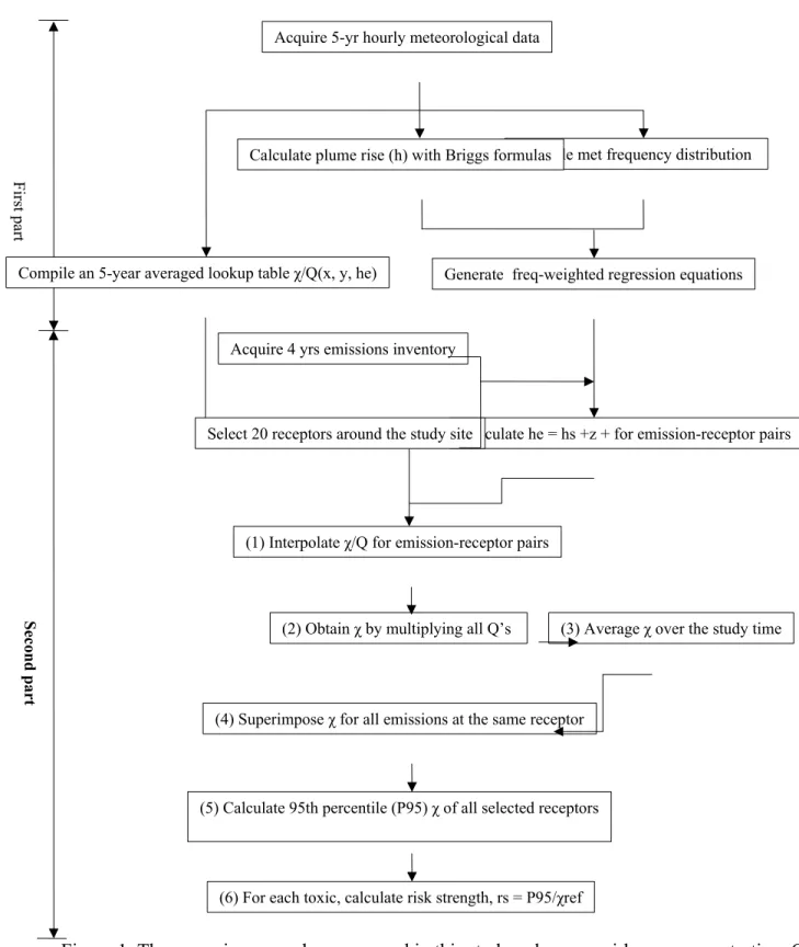
By the governing equation of dispersion factor derived in Section 2.2, the screening procedure for chronic exposure scenarios is illustrated in Fig. 1. The entire procedure consists of two parts. In the first part, 5-year hourly meteorological data to a study site is acquired. With the applicable range of effective release height (he) (0 to 300 meters), hourly ^χ /Q values are calculated beforehand by Eqs. 4 and 5 for all directions of winds (16 sectors) at several downwind distances (100 to 10000 meters). The results are compiled to form a 5-year averaged lookup table χ /Q (x , y , h^e) _. At the same time, taking several applicable ranges of distance, stack height, and buoyancy flux, frequency- weighted plume rises are calculated with Eq. 6 and the results are regressed to linear equations of ^{Δh (x , F´} b, h_s) _.

In the second part, four years of emission inventory representative to the study site are acquired. Prepare each selected emission-receptor pair of x and y coordinate and he

(=hs + ^Δh´ + Δ z), and proceed 6 steps of procedure below as illustrated in Fig. 1:

(1) Interpolate χ /Q for each selected pair from the χ /Q lookup table. To accommodate the large range of χ /Q over distance, a log interpolation of χ /Q is used.

(2) Obtain ^χ by multiplying each associated Q from the emission inventory over the study time with the interpolated ^χ /Q.

(3) Average χ over the study time.

(4) Superpose ^χ for all emissions at the same receptor.

(5) Calculate the mean and 95^th percentile (P95) χ of all the selected receptors.

(6) For each air toxic, calculate the mean and P95 of risk strength rs with Eq. 1.

2.5. The Industrial Complex Site Under Study

To demonstrate the screening procedure, Taichung site of Central Taiwan Science Park (CTSP), one of the 13 high-tech parks in Taiwan, was chosen. The Taichung site is one of the world-leading high-tech industrial complex of semi-conductors, electronics and electrical peripherals with a total investment over USD 25 billions (CSPA, 2008;

IDB, 2014). Beside the conventional pollutants (NO2, SO2, PM10, O3), the concerned pollutants emitted from the site are inorganic acidic (HF, HCl, NHO3, H2SO4) and basic (NH4OH) chemicals associated with cleaning and etching processes. Figure 2 is the site map of a total area of 413 hectares. Connected to the east-south is the Greater Taichung Metropolitan having 1.5 million of population. Around the site, Taichung Industrial Park, a conventional machinery industry complex being operated for over 3 decades, is located at 5 km south; Taichung Refuse Incinerator at 3 km southwest; Highway 1 at 2 km east; and Taichung Coal-burned Power Plant at 15 km east. Surrounded by these major potential sources of air emissions, Taichung site was characterized by high levels of background acidic and basic air pollutants during the low speed of southern wind in summer (Chen et al., 2010). The topography of the site is characterized by a low altitude terrain of 50-300 meters above the sea level, declining from northwest to southeast. On the map of Fig. 2, 20 representative locations were selected for this study, in which 10 inner receptor locations (D1 to D10) were of concerned by publics for regular monitoring stations (e.g. primary schools, nursing home, residential buildings), and 10 outer receptor

locations (TC1 to TC10) covering about 10 km range as required by TEPA (2011) for health risk assessment. For the 10 outer receptor locations, more stations were selected in the eastern and northeastern part of Taichung downtown area.

3. Results and Discussions 3.1. Meteorological Data

Five consecutive years (2006-2010) of hourly meteorological data, as recommended by TEPA in 2011 Risk Assessment Technical Guideline for chronic exposure scenarios, were obtained from the Taichung Weather Station for this study. Figure 3 shows the 16- directions of windrose for 5 years. The prevalence wind was primarily north wind in winter with a total frequency slightly less than 15%, in which approximately 5% and 8%

were associated with the two low wind speed categories of 1.0-2.0 m/s and 2.0-4.0 m/s, respectively. The results of frequency distribution for 6 stability class and 5 wind speed categories show that the highest frequency of 29% appeared at stability class 5 and low wind speed 2 m/s of the least dispersion condition.

3.2. Inventory Check and Hazard Identification

From the inventory check of Taichung Stationary Emission Database (TEPA, 2012a), a total of 1,654 emission records of 21 pollutants emitted from 232 stacks were identified for the Taichung site from 2007 to 2009. Based on the above inventory check, two tables were compiled in this study: stack parameter table and emission inventory table. Among the 21 pollutants, volatile organic chemical (VOC), PM10, and dust, are aggregate

pollutants and were eliminated from further analysis due to lack of reference data. Table 1 lists the rest of 18 pollutants for screening analysis, in which carbon monoxide (up to 192 tons/yr), nitrogen oxide (up to 27.06 tons/yr), and methylbenzene (up to 40.2 tons/yr) emitted at much higher rates than the rest. There were 9 acids and bases identified, in which sulfuric acid emitted at a much higher rate up to 16.31 tons/yr. Four criteria pollutants of CO, SO2, NO2, Pb were also identified.

There are two types of references identified for this study: reference concentration (RfC) and site boundary standard (Sb). Traditionally, the more formal hazard quotient (HQ) relative to reference concentration (RfC) is used for assessing non-carcinogenic risk in chronic exposure scenario. However, only 9 RfC values could be found in EPA (2013b) Integrated Risk Information System (IRIS) and DOE (2013) Risk Assessment Information System (RAIS) databases. Therefore, the site boundary standards (Sb) from Emission Standards of Stationary Pollution Sources (TEPA, 2013) were chosen as the reference for this study to evaluate rs. For the 4 criteria pollutants, ambient air quality standards (TEPA, 2012b) were used as the reference instead. It could be seen from Table 1 that arsine and phosphine are the two most health-concerned air toxics with the site boundary standards in the order of 10^-3 mg/m³, comparing with chlorine gas, hydrofluoric acid, leads, phosphoric acids, sodium hydroxide, sulfuric acid and sulfuric acid droplet in the order of 10^-2 mg/m³.

3.3. Plume Rise Regression Formulas

The plume generally rises to equilibrium after a few hundred meters of downwind distance. Accordingly, the frequency-weighted heights of plume rises were linearly regressed into two best-fit formulas on downwind distance x, stack height hs, and buoyancy flux Fb as below:

Δh=´

{

66 .5+3 . 45× 10⁻⁵x−0 . 734 h_s+1 . 99 F_bfor x ≤ 300 m

x >300 mEquation7

The R² values show fair linearity for both equations with slightly better linearity (0.8678 vs. 0.9536) for the long distance with much more observations (495 vs. 1320).

The average plume height is linearly proportional to x and Fb, but inversely proportional to hs. Within the 300 m near-range, transitional plume rise may occur and the regression yields a higher relative error for the intercept (7% vs. 2%). Comparing with the values of intercepts, the much smaller coefficients of x suggests insignificant contribution to the prediction plume heights for the long range. Also, its high p-value supports the high

likelihood of zero coefficients for x, and accordingly, x could be reasonably eliminated from the regression formula.

3.4. Calculated ^χ /Q

When looking into a general steady-state doubled Gaussian plume mathematical equation on which most air dispersion modeling is based, dispersion coefficients and emission rates are the two major variables affecting the modeling results. For the application of chronic exposure scenarios, dispersion coefficients are associated with long-term meteorological data and emission data with a representative operation in a period of time. As illustrated in the screening algorithm in Fig. 1, the first part is the most computationally intensive due to significant data crunching. With the pre- calculated χ /Q lookup table and the regression formulas for plume rise, the second part of χ /Q estimation at selected emission-receptor pairs can be significantly simplified. For the screening procedure developed in this study, the following mechanisms in the Gaussian plume formula are not considered: dry deposition, wet deposition, and chemical reaction. Consequently, the predicted values of χ /Q and rs

will be conservatively estimated.

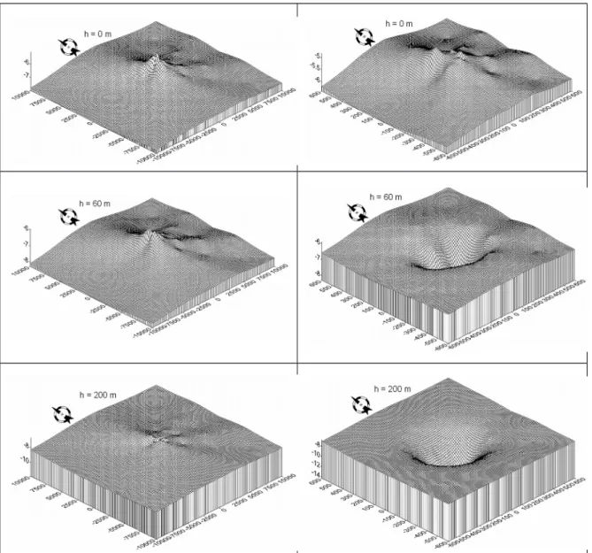
Two important intermediate results before the final calculating of rs are two tables:

χ /Q lookup table and frequency-weighted plume rise regression formula. As shown in Fig. 4, the result of 3-D wireframe plots of logarithmic ^χ /Q over a range of x and y distances at 3 effective release heights (he) of he of 0, 60, 200 m were compared on x and y Cartesian coordinates up to +/- 10 km. In order to examine the detailed changes, the distance scale was zoomed in to +/- 600 m where the changes were more significant. A significantly steep change around the release origin within a few hundred meters was observed even on the log scale of ^χ /Q. Beyond the first kilometer, the changes became relatively small for all release heights.

After comparing the values of χ /Q with different effective plume heights (he) on the scale of +/- 10 km in Fig. 4, there was a trend showing that the lower the he, the higher the χ /Q plateau ranging from 10^-8 to 10^-5 s/m³, which followed the Gaussian

dispersion theory. As for the zoomed in scale of +/- 600 m, interestingly, the predicted χ /Q results of the two higher he showed the depressed patterns around the origin while the result of he = 0 m showed the elevated pattern. It should be noted that the predicted χ /Q results were site-specific to emission characteristics and meteorological conditions. Furthermore, when using the χ /Q table, only he and x-y coordinates of interest are required to estimate χ /Q values from the contour plots of the study site in Fig. 4.

In this study, all the calculations were programmed in MS Excel with dispersion equations. Alternatively, the χ/Q lookup table and regression formulas could also be generated by other acceptable methods, such as ISCST3, GENII, AERMOD, or any regulatory complied dispersion codes. Although more sophisticated built-in mechanisms of dispersion can be utilized in those computer codes; yet, the procedure is still applicable with little or no modification because the procedure following the lookup table and regression is essentially just an interpolation algorithm. To validate the procedure and double check the results, the same set of meteorological data and emission inventory were used in the TEPA’s recommended ISCST3. The average concentration at the 20 receptor locations is 19% less than that of the screening procedure (the results from the procedure are conservative). If considering only the inner locations (D1 to D10), the ISCST3’s average is only 6.7% less. Regardless the simplifying approach used in this study, the results show reasonable accuracy and reliable consistency with the full-strength industrial dispersion code. In addition, the Excel implementation in this study

demonstrated to be flexible to accommodate various data sets and equations, and is transparent and traceable on step-by-step calculation.

3.5. Ranking Results

Figure 5 gives the ranking results of 10 air toxics in this study. The rs values were in the range of 10^-2-10^-4 for 95^th percentile (P95) and 10^-2-10^-5 for mean of the 20 selected locations. The P95 as an upper bound was used to be protective to most general public residing around the site for a chronic scenario (TEPA, 2011). The top four pollutants in P95 were nitrogen dioxide, hydrogen fluoride, chlorine, and sulfuric acid drop, in which

the last three were directly associated with the industrial activities and could be served as the indicating air toxics required for intensive monitoring and further analysis. The highest rs was located at D6 for nitrogen dioxide on northwest boundary of the Taichung site, about 100 m away from the nearest release point. As shown in Fig. 3, this hot spot could be expected due to predominated southeast wind.

Although VOC as an aggregate pollutant was not included in Table 1, 15 individual VOC chemicals were identified to have significant ambient increases in the neighborhood around the Taichung site (CSPA, 2008). However, the emission sources around this area are fairly complicated (see Section 2.5). Among the 15 VOC chemicals, xylene and toluene were listed in Table 1. If all the VOC chemicals were summed together for screening, the 95^th-percentiled rs value of VOC will be ranked in the top 5.

The lookup table for χ/Q and the regression formulas for Δ h are created beforehand using 5 years of hourly metrological data to cope with the two most computation-

intensive steps with Eqs. 4 to 7. The table and formulas are pre-created to decouple the release-receptor data from the meteorological data. After creation, the table and

regression formulas could be considered as a long-term steady dispersion system for the site-specific environmental settings. Even with different sets of emission data in different years of release inventory for retrospective or perspective prediction, different receptor locations, or different regulated pollutants, the same screening procedure can be applied with little or no modification. Although the demonstration in this study is based on simple point sources, the χ/Q interpolation could be readily extended to complicated large area sources (Yuan, Wang, and Zielen, 1988).

4. Conclusions

To meet regulatory requirements for ever-increasing airborne pollutants of the high- tech science parks, this screening procedure was developed in this study to provide a practical yet sufficiently accurate approach. With the operationally defined risk strength, and the design of χ/Q lookup table and regression formulas, the screening procedure is valuable to allow for the screening of critical pollutants with various long-term exposure

scenarios and applications. The procedure is particularly advantageous to in-house decision as the decoupling of extensive Gaussian plume calculations with meteorological data from tremendous arrays of emission data.

Acknowledgments

We appreciate the financial supports from Taichung Bureau of Environmental Protection under the contract of N0176-2012 and National Environmental Health Research Center, National Health Research Institute (NHSI), Taiwan under the contract of NRSI-EH-102-PP12 and NRSI-EH-103-PP12.

References

Briggs, G.A., 1975. Chapter 3, Plume Rise Predictions, pp. 59-111 in Lectures on Air Pollution and Environmental Impact Analysis. (Duane A. Haugen, Ed.) American Meteorology Society, Boston, MA.

Chen, H.W., Tsai, C.T., She, C.W., Lin, Y.C., Chiang, C.F., 2010. Exploring the

background features of acidic and basic air pollutants around an industrial complex using data mining approach. Chemosphere. 81:1358-1367.

Chiang, C.F., Tsai, C.T., 2014. Establishment and testing of a regional air quality management decision-making support system—A case study of particulate pollutants in Taichung City, Proceeding of 4^th Mainland-Taiwan Environmental Protection Conference, Fuzhou Forum, Fuzhou City of Fujian Province, August 18- 19, 2014.

CSPA, 2008. Preliminary Operating Quality Assurance Planning of Volatile Organic Compound Monitoring Station of Central Taiwan Science Park, Central Science Park Administration (CSPA) of Taiwan National Science Council, Taipei, Taiwan.

DOE, 2013. Risk Assessment Information System. Office of Environmental

Management, U.S. Department of Energy (DOE). Accessed on October 18, 2013, http://rais.ornl.gov/tools/metadata.php.

EPA, 1989. Risk Assessment Guidance for Superfund Volume I: Human Health Evaluation Manual (Part A), EPA/540/1-89/002, U.S. Environmental Protection Agency (EPA).

EPA, 1995. User’s Guide for the Industrial Source Complex (ISC3) Dispersion Models, Volume II—Description of Model Algorithm, EPA-454/B-95-003b, U.S. EPA.

EPA, 2013a. Dose-Response Assessment for Assessing Health Risks Associated With Exposure to Hazardous Air Pollutants. U.S. EPA. Accessed on October 3, 2013, http://www.epa.gov/ttn/atw/toxsource/summary.html.

EPA, 2013b. Integrated Risk Information System (IRIS). U.S. EPA. Accessed on October 10, 2013, http://www.epa.gov/IRIS/.

EPA, 2013c. The HEM-3 User’s Guide. Instructions for Using the Human Exposure Model Version 1.3.0 (AERMOD version) for Single Facility Modeling. U.S. EPA.

IDB, 2014. Taiwan Industrial Parks Supply and Service Information Web. Industrial Development Bureau (IDB), Ministry of Economic Affairs, Taiwan. Accessed on January 25, 2014, http://idbpark.moeaidb.gov.tw/Environ/Default.

Ma, H.W., Shih, H.C., Hung, M.L., Chao, C.W., Li, P.C., 2012. Integrating input output analysis with risk assessment to evaluate the population risk of arsenic. Environ. Sci.

Technol. 46, 1104−1110.

Napier, B.A., Strenge, D.L., Ramsdell, Jr. J.V., Eslinger, P.W., Fosmire, C., 2011. GENII Version 2 Design Document, Pacific Northwest National Laboratory, PNNL-14584 Rev. 3.

TEPA, 2011. Technical Guides of Health Risk Assessment. Taiwan Environmental Protection Administration (TEPA), Taipei, Taiwan.

TEPA, 2012a. Emission Database of Stationary Pollution Sources of Taichung City.

TEPA, Taipei, Taiwan.

TEPA, 2012b. Air Quality Standard. TEPA. Revised and Promulgated on May 14, 2012.

Taipei, Taiwan.

TEPA, 2013. Emission Standards of Stationary Pollution Sources, TEPA. Revised and Promulgated on April 24, 2013. Taipei, Taiwan.

Turner, D.B., 1994. Workbook of Atmospheric Dispersion Estimates (2^nd Ed.). CRC Press, New York.

Yuan, Y.C., Wang, J., Zielen, A., 1988. MILDOS-AREA: An Enhanced Version of MILDOS for Large-Area Sources, ANL/ES-161.

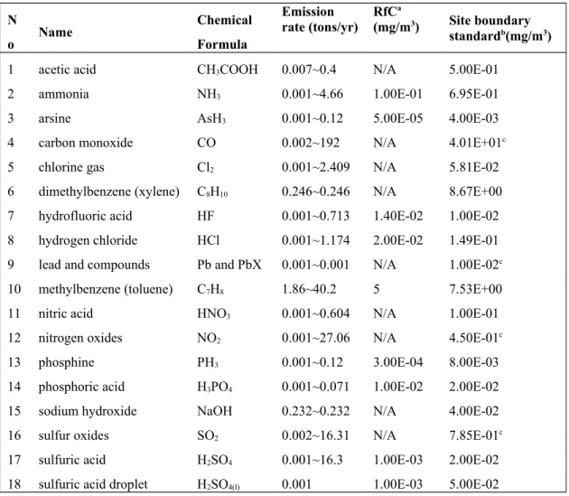
Table 1. Results of inventory check of airborne pollutants from the emission database in 2007-2010 of the Taichung site in this study.

N

o Name Chemical

Formula

Emission

rate (tons/yr) RfC^a

(mg/m³) Site boundary standard^b(mg/m³)

1 acetic acid CH3COOH 0.007~0.4 N/A 5.00E-01

2 ammonia NH3 0.001~4.66 1.00E-01 6.95E-01

3 arsine AsH3 0.001~0.12 5.00E-05 4.00E-03

4 carbon monoxide CO 0.002~192 N/A 4.01E+01^c

5 chlorine gas Cl2 0.001~2.409 N/A 5.81E-02

6 dimethylbenzene (xylene) C8H10 0.246~0.246 N/A 8.67E+00

7 hydrofluoric acid HF 0.001~0.713 1.40E-02 1.00E-02

8 hydrogen chloride HCl 0.001~1.174 2.00E-02 1.49E-01

9 lead and compounds Pb and PbX 0.001~0.001 N/A 1.00E-02^c 10 methylbenzene (toluene) C7H8 1.86~40.2 5 7.53E+00

11 nitric acid HNO3 0.001~0.604 N/A 1.00E-01

12 nitrogen oxides NO2 0.001~27.06 N/A 4.50E-01^c

13 phosphine PH3 0.001~0.12 3.00E-04 8.00E-03

14 phosphoric acid H3PO4 0.001~0.071 1.00E-02 2.00E-02

15 sodium hydroxide NaOH 0.232~0.232 N/A 4.00E-02

16 sulfur oxides SO2 0.002~16.31 N/A 7.85E-01^c

17 sulfuric acid H2SO4 0.001~16.3 1.00E-03 2.00E-02 18 sulfuric acid droplet H2SO4(l) 0.001 1.00E-03 5.00E-02

aIntegrated Risk Information System (EPA, 2013b) and Risk Assessment Information System (DOE, 2013).

bEmission Standards of Stationary Sources (TEPA, 2013)

cAmbient Air Quality Standards (TEPA, 2012b)

Second partFirst part

(1) Interpolate χ/Q for emission-receptor pairs

(3) Average χ over the study time

(6) For each toxic, calculate risk strength, rs = P95/χref (4) Superimpose χ for all emissions at the same receptor

(2) Obtain χ by multiplying all Q’s

(5) Calculate 95th percentile (P95) χ of all selected receptors

Compile met frequency distribution Calculate plume rise (h) with Briggs formulas

Acquire 5-yr hourly meteorological data

Generate freq-weighted regression equations Compile an 5-year averaged lookup table χ/Q(x, y, he)

Calculate he = hs +z + for emission-receptor pairs Acquire 4 yrs emissions inventory

Select 20 receptors around the study site

Figure 1. The screening procedure proposed in this study, where χ = airborne concentration, Q

= emission rate, χref = site boundary standard, hs = stack height, Δ z = elevation difference, Δh = frequency weighted plume rise, h´ e = effective plume height.

Figure 2. Map of the high-tech industrial complex, showing 10 inner receptor locations (D1-D10) of regular monitoring stations, and 10 outer receptor locations (TC1-TC10) covering about 10 km range required by TEPA for health risk assessment.

Figure 3. Sixteen directions and five wind speeds of windrose for 2006-2010 hourly data for the study site.

Figure 4. Results of 3-D wireframe plots of predicted logarithmic average /Q of 5 years (2006-2010) of hourly metrological data at 3 effective release heights (0, 60, 200 m) for the Taichung site, left plots covering up to 10 km, right plots covering the close-up to 600 m to show detailed changes in logarithm z scale of /Q around the source in the center.

Figure 5. Screening results of mean and 95^th percentile rs values for the ten highest values of the 20 receptor locations selected for the Taichung site.