A Graph Neural Network Assisted Monte Carlo Tree Search Approach to Traveling Salesman Problem
ZHIHAO XING AND SHIKUI TU , (Member, IEEE)
Department of Computer Science and Engineering, Shanghai Jiao Tong University, Shanghai 200240, China
Centre for Cognitive Machines and Computational Health (CMaCH), School of SEIEE, Shanghai Jiao Tong University, Shanghai 200240, China Corresponding author: Shikui Tu ([email protected])
This work was supported by the National Science and Technology Innovation 2030 Major Project of the Ministry of Science and Technology of China under Grant 2018AAA0100700, in part by the Zhi-Yuan Chair Professorship Start-up Grant from Shanghai Jiao Tong University under Grant WF220103010.
ABSTRACT We tackle the classical traveling salesman problem (TSP) by combining a graph neural network and Monte Carlo Tree Search. We adopt a greedy algorithm framework to derive a promising tour by adding the vertices successively. A graph neural network is trained to capture graph motifs and interactions between vertices, and then to give the prior probability of selecting a vertex at every step. Instead of making decisions directly based on the output of graph neural networks, we combine the graph neural network with Monte Carlo Tree Search to provide a more reliable policy as the output of the latter is the feedback information by fusing the prior probability with the scouting exploration. Without much heuristic designing, our approach outperforms recent state-of-the-art learning-based methods on the TSP. Experimental results demonstrate that the proposed method can be generalized to instances with more vertices than those used during the training.
INDEX TERMS Combinatorial optimization problem, deep neural network, graph neural network, Monte Carlo tree search, reinforcement learning, traveling salesman problem.
I. INTRODUCTION
The Traveling Salesman Problem (TSP) is a classical com- binatorial optimization problem, which has many practical applications in real life, such as planning, manufacturing, and genetics [1]. The goal of the TSP is to find the shortest route that visits each city exactly once and ends in the origin city, which is well-known as an NP-hard problem [2]. To solve the TSP, many approximation algorithms have been pro- posed [3], [4], among which the heuristic search algorithms get prevalence by finding a satisfactory solution within a rea- sonable time cost. However, the performance of the heuristic algorithms depends on heuristics handcrafted to guide the search to find competitive tours efficiently [5], [6]. Moreover, the design of heuristics usually requires substantial expertise on the problem.
Recent advances in deep learning provide a powerful way of learning effective representations from data, leading to breakthroughs in many fields, such as image segmentation [7]
and speech recognition [8]. Efforts have been made to tackle
The associate editor coordinating the review of this manuscript and approving it for publication was Huiyu Zhou.
the TSP by the deep learning approach by avoiding hand- crafted feature extraction and design of heuristics [9]–[11].
In another work, Dai et al. [12] stated above neural architec- tures cannot yet effectively reflect the graph structure of the TSP and proposed a graph embedding architecture to capture graph properties. Recently, some researchers have observed that the graph neural network (GNN) can be used to discover useful patterns of graph-based combinatorial problems and showed that GNN can find universal motifs that are present in graphs of different scales [13]–[16].
While solving the TSP, most current learning-based meth- ods derive a tour by directly selecting vertices with a pre- defined large probability to the output of deep neural net- works [9]–[12], [17]. Hence, the decision may not be reliable as such a learning based method has only one chance to compute the optimal tour and it never goes back to reverse the decision. Recently, some works [15], [18] show that the combination of deep neural networks and tree search could make a more reliable decision than that made using the output of neural networks only. Li et al. [15] proposed an approach for solving four different types of NP-hard problems by converting them into the equivalent maximal independent set
This work is licensed under a Creative Commons Attribution 4.0 License. For more information, see https://creativecommons.org/licenses/by/4.0/
(MIS) problem. The proposed method first predicts multiple probability maps and then exploits a breadth-first tree search to rapidly generate a large number of candidate solutions for the MIS problem. Silver et al. [18] proposed a Go program, called the AlphaGo, and made remarkable achievements in the Go game. An important factor for the success of the AlphaGo is the combination of deep convolutional neural networks (CNN) and Monte Carlo Tree Search (MCTS) [19], [20], which exploits neural networks in the evaluation of board positions and effectively reduces the search space of the tree. However, such AlphaGo-like systems cannot be applied directly to the TSP due to three major differences between the TSP and the Go game. Firstly, a 2D image representing an explicit board of states for the TSP is difficult to formulate in the Go game. Secondly, there is no efficient and accurate heuristic for evaluating the TSP. Finally, the AlphaGo tracks the average winning rate of each branch to guide moves, while the TSP requires to find the extreme without keeping any sense to the average value which may also include several suboptimal routes surrounding the extreme route.
In recent years [21]–[23], it is recommended and also further addressed to combine AlphaGoZero type techniques and the classic heuristic search mechanisms (CHSMs) for the combinatorial optimization problems such as TSP and graph matching. On one hand, one uses deep neural net- works to estimate heuristics in use of CHSMs via learning from samples. On the other hand, one borrows concepts and mechanisms used in CHSMs into AlphaGoZero for further improvements. To the purpose, a family of deep IA-search methods was proposed in [21] based mainly on combining AlphaGoZero, A∗ search, and CNneim-A [24]. This deep IA-search is developed under the framework of deep bidi- rectional intelligence via YIng YAng (IA) system, which is featured by circling A-mapping by deep neural network learning and I-mapping by solving searching, as illustrated in Fig. 15 of [22]. Moreover, constrains encountered in TSP and graph matching are tackled by an IA-DSM scheme [22], [23], together with a feature enrichment technique [21].
A preliminary effort was recently made on TSP in [25] to perform an improvement of one algorithm in the above deep IA-search family. Specifically, V-AlphaGoZero in Table 1 of [21] is improved with deep neural networks implemented by a graph embedding network (GEN) [12], which is shortly named as GEN-MCTS with AlphaGoZero replaced by its core MCTS because we also need to modify some detailed implementations suitable for merely GO. Interestingly, promising results come in solving TSP problems of small- to-medium sizes [25]. Here, we further propose to replace the GEN part by GNN because several efforts [13]–[16]
demonstrated promising uses of GNN even without MCTS.
In other words, GEN-MCTS is extended into GNN- MCTS, featured by three improvements. First, it improves implementing the A-mapping in estimating the prior prob- ability for each vertex as its output. Second, while prior probabilities are used for tree search in a way similar to ones in AlphaGoZero or V-AlphaGoZero in [21], it improves the
I-mapping with the lookahead scouting mechanism behind CNneim-A [24] adopted here for re-estimating heuristics in updating Q-values, somewhat like a variant of DCA-E in Table 1 of [21]. Third, instead of memorizing the average action value, we track the best action value found under the subtree of each node for determining its exploitation value as suggested in [26] in the context of the stock trading problem.
In 2D Euclidean graphs having up to 100 vertices, our method could outperform other learning-based approaches in the greedy framework, and it could also reach close to the optimal solutions. Furthermore, experimental results on large-scale the TSP instances demonstrate that the proposed method could perform better than other learning-based meth- ods even if trained on the small-scale instances. The results suggest that our method is promising to solve combinatorial optimization problems like the TSP.
The remainder of the paper is organized as follows: After reviewing related works in SectionII, our approach is for- mulated in Section III. Experimental results are presented in SectionIV, followed by the conclusion of the article in SectionV.
II. RELATED WORK
The TSP is a well studied combinatorial optimization prob- lem, and there are various ways to solve this problem.
Since our work follows the line of a learning-based method, we restrict the literature survey only to the development of various representative strategies used in the learning-based methods.
In 1985, Hopfield et al. [27] proposed a neural network to solve the TSP for the first time. After that, researchers made many efforts to propose neural network based various methods and also to improve their performances [28]–[33].
With the development of deep leaning in recent years, deep neural networks have been adopted to solve the TSP also and achieved remarkable results.
Vinyals et al. [9] proposed an architecture, called the Pointer Net (Ptr-Net), to learn the conditional probability of a tour using a mechanism of neural attention [34] in a super- vised way. Instead of using attention to blend hidden units of an encoder to a context vector, they used the same (atten- tion) as pointers to the input vertices. During testing, they used a beam search procedure to find the best possible tour.
Two flaws exist in that method. Firstly, the Ptr-Net can be applied to solve small scale (n ≤ 50) problems only. Secondly, the beam search procedure might generate invalid routes also.
On the basis of the work in [9], Bello et al. [10] employed the PtrNet as a policy model to learn a stochastic policy over tours. Furthermore, they masked the visited vertices to avoid deriving invalid routes and added a ‘‘glimpse’’
which aggregates different parts of the input sequence to improve the performance of the method. Instead of training the model in a supervised way, they introduced an actor- critic algorithm [35] to learn the parameters of the model and empirically demonstrated that the generalization is better compared to optimizing a supervised mapping of labeled
VOLUME 8, 2020 108419
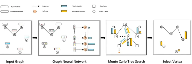
FIGURE 1. Approach overview. First, the graph is fed into the graph neural network, which captures graph characteristics and interactions between vertices, and then generates a prior probability that indicates how likely each vertex is in the tour sequence. Then, with the assistance of the graph neural network, a developed MCTS outputs an improved probability by scouting simulations. Lastly, we visit the best vertex among unvisited vertices according to the improved probability. The above process will loop until all vertices are visited. Best viewed in color.
data. The algorithm significantly outperformed the super- vised learning approach [9] with up to 100 vertices.
Kool et al. [11] introduced an efficient model and a training method to improve the above stated learning-based heuristics for routing problems. Compared to [10], they could reduce the influence of order in which vertices are fed into the neural network by replacing recurrence (LSTMs) with attention lay- ers [36]. They also applied a reinforcement learning method to train the model. Instead of learning a value function as a baseline, they introduced a greedy rollout policy to generate a baseline of improved quality and also to improve the conver- gence speed of the approach. They improved the state-of-art performance for 20, 50, and 100 vertices. Deudon et al. [17]
also proposed a framework, different from the work of Kool et al. [11], which uses attention layers and the reinforce- ment learning algorithm (actor-critic) to learn a stochastic policy. They combined the machine learning methods with the existing 2-opt heuristic algorithm to enhance the perfor- mance of the framework.
However, as stated in [12], the above mentioned neural architectures cannot yet effectively reflect the graph structure of the TSP. Furthermore, Dai et al. [12] considered the TSP as a graph, and proposed a framework which combines reinforcement learning with graph embedding neural net- work to construct solutions incrementally for the TSP and other combinatorial optimization problems. They introduced a graph embedding network based on the structure2vec [37]
to capture the current state of the solution and the structure of a graph. Then, they used Q-learning parameterized by the graph embedding network to learn a greedy policy that will decide which vertex is to be inserted into the partial tour. They adopted the farthest strategy [38] to get the best insertion position in the partial tour.
Besides graph embedding [12], graph neural net- work (GNN) is broadly used to solve graph-based problems.
Recently, some researchers have observed that GNN can be used to discover useful patterns of the TSP [13], [14], [39]
and other graph-based combinatorial problems [15], [16], and
showed that GNN can find universal motifs that are present in graphs of different scales.
Inspired by the success of GNN on combinatorial opti- mization problems, we train a developed GNN to represent the features of the TSP in a better way. Since the output of the MCTS is the feedback information by fusing the prior probability with the scouting exploration, we combine the GNN with MCTS to get more reliable decisions.
III. PROPOSED APPROACH
Let G(V, E) denotes a weighted graph, where V is the set of vertices, and E is the set of edges. Also, let e(u, v) is the weight of edge (u, v) ∈ E, where u, v ∈ V . We use S = {v1, v2, . . . , vi}to represent a tour sequence that starts with v1and ends with vi, and ¯S = V \ Sis the set of candidate vertices for addition to S.
Given the graph G(V, E) or simply G, our goal is to derive a tour by adding vertex v ∈ ¯Sto S in turn. A natural approach is to train a deep neural network to predict which vertex is to be added to the partial tour sequence at a particular step. That is, neural network f (G|S) will take graph G and partial tour sequence S as input, and return probabilities of the vertices indicating the likeliness of each vertex to get selected. For the TSP, both the structural patterns of the graph and the state of the vertices can become very complex to be described.
To represent such a complex context, we will leverage the graph neural network (GNN) [40] to parameterize f (G|S).
Intuitively, we can directly use the prior probability to a vertex, e.g., selecting a vertex with the highest probability, to generate the tour sequence incrementally. However, deriv- ing tours in this way might not be reliable as a learning based algorithm has only one chance to compute the optimal tour, and it never goes back to reverse the decision. To overcome this drawback, we combine the graph neural network with the Monte Carlo Tree Search [19], [20] to get a better policy.
On one hand, we use a variant of PUCT [41] to balance exploration (i.e., visiting a state as suggested by the prior policy) and exploitation (i.e., visiting a state that has the
best value). Using the concept of prior probability, the search space of the tree could be reduced substantially, enabling the search to allocate more computing resources to the states having higher values. On the other hand, we could get a more reliable policy after a large number of simulations as the output of the Monte Carlo Tree Search acts as the feedback information by fusing the prior probability with the scouting exploration. The overall approach is illustrated in Fig.1.
A. DEEP NEURAL NETWORK ARCHITECTURE
To get a good network, information about the structures of the concerned graph and contextual information, i.e., tour sequence S = {v1, . . . , vi}, is required. We tag vertex v with xv = 1 if it is already visited, otherwise xv =0. Intuitively, f(G|S) should summarize the state of such a ‘‘tagged’’ graph and generate the prior probability for each vertex to get included in S.
Unlike in other graph-based combinatorial optimization problems such as the Maximal Independent Set (MIS) and Minimum Vector Cover (MVC) [15] as stated in [12], we have not ignored edge features as the objective of the TSP is com- puted based on the edge cost, i.e., the distance between two vertices. Hence, we have modified the basic GNN [40], which we call the static edge graph neural network (SE-GNN), to efficiently extract node and edge features of the TSP.
1) GRAPH NEURAL NETWORK
A GNN model consists of a stack of T neural network layers, where each layer aggregates local neighborhood information, i.e., features of neighbors of each node, and then passes this aggregated information to the next layer. We use Hvt to denote the real-valued feature vector associated with node vat layer t. Specifically, the basic GNN model [40] can be implemented as follows. In layer t = 1, 2, . . . , T , a new feature is computed as given by (1).
Hvt+1=σ
HvtW1t+ X
u∈N(v)
HutW2t
(1)
In (1), N (v) is the set of neighbors of vertex v, W1t and W2t are the parameter matrices for the layer t, andσ(·) denotes a component-wise non-linear function such as a sigmoid or a ReLU function. For t = 0, Hv0 denotes the feature initialization at the input layer.
As can be observed in (1), the edge information is not taken into account. There are many ways to integrate edge features. Gilmer et al. [42] considered the edge information as a kind of metric to measure the usefulness of the neighbors of a node, while Dai et al. [12] and Xie and Grossman [43]
took edge features as independent parts and integrated them with node features. Since the edge information in the TSP is important, we adopt the ways presented in [12], [43]. Accord- ingly, edge features can be integrated with node features using (2) [12].
µt+1v =σ
θ1xv+θ2
X
u∈N(v)
µtu+θ3
X
u∈N(v)
σ(θ4w(v, u))
(2)
In (2),θ1 ∈ Rl,θ2, θ3 ∈ Rl×l andθ4 ∈ Rl are all model parameters.
We can see in (1) and (2) that the nonlinear mapping of the aggregated information is a single-layer perceptron, which is not enough to map distinct multisets into unique embeddings.
Hence, as per the suggestion in [44], we replace the single perceptron with multi-layer perceptron. Finally, we compute new node feature H using (3).
Hvt+1=MLPt
HvtW1t+ X
u∈N(v)
HutW2t+ X
u∈N(v)
ev,uW3t
(3) In (3), e(v, u) is the edge feature,1W3tare parameter matrices, and MLPtis the multi-layer perceptron for the layer t.
Note that SE-GNN differs from GEN [12] in the following aspects: 1) SE-GNN replaces xv in (2) with Hv so that the SE-GNN can integrate the latest feature of the node itself directly. 2) each update process in the GEN can be treated as one update layer of the SE-GNN, i.e., each calculation is equivalent to going one layer forward, thus calculating T times for T layers. Parameters of each layer of SE-GNN are independent, while parameters in GEN are shared between different update processes which limits the ability of the neural network. 3) We replaceσ in (2) with MLP as suggested by [44] for helping neural networks to map distinct multisets to unique embeddings.
We initialize the node feature H0as follows. Each vertex has a feature tag which is a 3-dimensional vector. The first element of the vector is binary and it is equal to 1 if the partial tour sequence S contains the vertex. The second and third elements of the feature tag are, respectively, the x and ycoordinate values of the vertex. The problem is to find a path from the last vertex to the first vertex, going through all the unvisited vertices. To know the first and last vertices in partial tour sequence S, we extend the node feature H0by adding feature tags of those vertices in S, besides the basic feature tags as described above.
2) PARAMETERIZING f (G|S;2)
Once the feature for every vertex is computed after updating T layers, we use the new feature for the vertices to define f(G|S;2) function, which returns the prior probability for each vertex indicating how likely the vertex will belong to partial tour sequence S. More specifically, we fuse all vertex feature HvT as the current state representation of the graph and parameterize f (G|S;2) as expressed by (4), where sum means summation.
f(G|S;2) = softmax(sum(H1T), . . . , sum(HnT)) (4) During training, we minimize the cross-entropy loss for each training sample (Gi, Si) in a supervised manner as given by (5).
`(Si, f (Gi|Si;Θ)) = −
N
X
j=1
yjlog f (Gi|Si(1 : j − 1);Θ) (5)
1Euclidean distance: given two points (x1, y1) and (x2, y2) in two- dimensional plane, D =p
(x2− x1)2+(y2− y1)2
VOLUME 8, 2020 108421
In (5), Si is a tour sequence which is a permutation of the vertices of graph Gi, and yjis a one-hot vector whose length is N and the S(j)-th position is 1.
B. GRAPH NEURAL NETWORK ASSISTED MONTE CARLO TREE SEARCH
Similar to the implementation in [18], the GNN-MCTS uses graph neural networks as a guide of MCTS. Each node s in the search tree contains edges (s, a) for all legal actions a ∈ A(s).
Each edge stores a set of statistics, {N(s, a), Q(s, a), P(s, a)}
where node s denotes the current state of graph including sequence S and other graph information, action a denotes the selection of vertex v from ¯S to S, N (s, a) is the visit count, Q(s, a) is the action value and P(s, a) is the prior probability of selecting edge (s, a).
It is to be mentioned that the following are three main differences between the TSP and the Go game:
• The Go game tracks the average winning rate of a branch of MCTS to guide moves [18]. However, the TSP is interested in finding the extreme, and hence the aver- age value makes no sense to it as several suboptimal routes may even surround the extreme route. Instead of recording the average action value, we track the best action value found under the subtree of each node for determining exploitation value of tree node as suggested in [26] in the context of the stock trading problem.
• In the Go game, it is common to use {0, 0.5, 1} to denote, respectively, the loss, draw, and win in a game. It is not only convenient, but it also meets the requirements of UCT [20] if reward lies in the range of [0, 1]. In the TSP, an arbitrary tour length can be achieved that does not fall in a predefined interval. One can solve this issue by adjusting the parameters of UCT in such a way that it is feasible for a specified interval. Adjusting parameters requires substantial trial-and-error due to the change in the number of vertices. Instead, we address this issue by normalizing the action value of node n, whose parent is node p, in the range of [0, 1] using (6).
Qn=Qn− wp bp− wp
(6) In (6), bpand wpare, respectively, the best (maximum) and the worst (minimum) action value under p, and Qnis the action value of n. The actions under p are normalized in the range of [0, 1] in such a way that the best action is normalized to 1 and the worst action to 0.
• AlphaGo uses a learned value function (critic) v(s, θ) to estimate the probability of the current player win- ning from position s, where parameter θ is learned from observation (s, π). However, in the TSP, such a learned value function has to tolerate the large range of value change between different solutions, while it is also expected to preserve the sensitivity to very small value change around the optimal solution. Thus, in our
Algorithm 1 Value Function
• start denotes the state of leaf node l
• Bdenotes the beam width
• Sdenotes the partial tour corresponding to a state.
1: Initialize beam = {start}
2: while beam 6= ∅ do
3: set = ∅
4: for each state s in beam do
5: for each successor state c of state s do
6: Compute value = P|S|
j=1log f (G|S(1 : j − 1) of the successor state c
7: set = set ∪ { successor state c }
8: end for
9: end for
10: beam = ∅
11: while set 6= ∅ and B < |set| do
12: Select state e in set with smallest value
13: Delete state e from set
14: end while
15: for each state s in set do
16: if state s is an end state then
17: Select state r in set with biggest value
18: Computer tour length corresponding to state r
19: return tour length
20: else
21: beam = beam ∪ { state s }
22: end if
23: end for
24: end while
view, the above reason makes the learned value func- tion hardly workable in the TSP. Instead, we design a non-learnable value function h(s) that combines the pre- trained GNN and the beam search to evaluate the pos- sible tour length from the current state to the end state.
Guided by the output of the pre-trained GNN, the value function executes the beam search from the state leaf corresponding to leaf node l until reaching an end state.
We set the value of leaf node l as Vl= −h(stateleaf). The value function is described in Algorithm1.
The GNN-MCTS proceeds by iterating over the four phases and then selects a move to play.
• Selection Strategy. The first in-tree phase of each rollout starts at the root of node s0of the search tree and finishes when the rollout reaches a leaf node sl at time step l. At time step t<l, we use a variant of PUCT [41]
to balance exploration (i.e., visiting the states as sug- gested by the prior policy) and exploitation (i.e., visiting the states which have the best value) according to the statistics in the search tree as given by (7) and (8), respectively, where cpuct is a constant to trading off between exploration and exploitation.
at =arg max
a (Q(st, a) + U(st, a)) (7)
U(s, a) = cpuctP(s, a) pP
bN(s, b)
1 + N (s, a) (8)
• Expansion Strategy. When a leaf node l is reached, the corresponding state sl is evaluated by the graph neural network to obtain the prior probability p of its children nodes. The leaf node is expanded and the statis- tic of each edge (sl, a) is initialized to {N(sl, a) = 0, Q(sl, a) = −∞,2P(sl, a) = pa}.
• Simulation Strategy. Rather than using a random strat- egy, we use value function h(s) to evaluate the length of the tour that may be generated from the leaf node l.
• Back-Propagation Strategy. For each step t < l, the edge statistics are updated in a backward process.
The visit counts are increased as N (st, at) = N (st, at) + 1, and the action value is updated to the best value as Q(st, at) = max(Q(st, at), Vl).
• Play. At the end of several rollouts, we select the node with the biggest ˆP(a|s0) = 1 −PQ(s0,a)
bQ(s0,b) as the next move a in the root position s0. The search tree will be reused at subsequent time steps: the child node relating to the selected node becomes the new root node, and all the statistics of sub-tree below this child node is retained.
IV. EXPERIMENTS A. EXPERIMENTAL SETUP 1) INSTANCE GENERATION
To evaluate our method against other approximation algo- rithms and deep learning-based approaches, we use an instance generator from the DIMACS TSP Challenge [45]
to generate two types of Euclidean instances: ‘‘random’’
instances consisting of n points scattered uniformly at random in the [106, 106] square; ‘‘clustered’’ instances consisting of n points that are clustered into n/100 clusters. We con- sider three benchmark instances, namely Euclidean TSP20, TSP50, and TSP100.
2) BASELINES
To compute the optimal solutions, we use two state-of-the-art solvers, Concorde3[46] and Gurobi4[47]. We compare our results with those of the Nearest, Random and Farthest Inser- tion, as well as Nearest Neighbor, which are non-learning baseline algorithms that also derive a tour by adding ver- tices successively. Additionally, we compare our results with those of the excellent deep learning-based methods based on the greedy framework as mentioned in SectionII, the most important of which are the methods of Vinyals et al. [9], Bello et al. [10], Kool et al. [11], and Dai et al. [12].
3) TRAINING AND TESTING
To train SE-GNN (settings are in SectionIV-E5), we generate 100,000, 40,000 and 20,000 instances for TSP20, TSP50,
2In the experiment, we initialize Q with -5.0, -10.0 and -15.0 for TSP20, TSP50, and TSP100, respectively.
3http://www.math.uwaterloo.ca/tsp/concorde/
4http://www.gurobi.com/
and TSP100, respectively. We use two state-of-art solvers (Gurobi and Concorde) to obtain the optimal tour for each instance. Then we generate samples for each instance accord- ing to the optimal tour sequence. We divide the dataset into a training set, a validation set, and a test set in the ratio of 8: 1: 1. We use Adam [48] with 512 mini-batches and a learning rate of 10−3. The training is conducted for 60 epochs on a machine with 2080ti GPU. After training models for TSP20, TSP50, and TSP100, respectively, we use the pre-trained SE-GNN to guide MCTS. During testing, we randomly generate 1000 instances for the above three models. The parameter settings of the GNN-MCTS used in our experiments are as follows: we set cpuct = 1.3 and beam width = 1 (more discussion is in SectionIV-E3); we set rollouts = 800, 800 and 1200 for TSP20, TSP50, and TSP100, respectively.
B. RESULTS
Besides non-learning algorithms, we compare our method with excellent deep learning-based works which derive tours using some greedy mechanisms. Results of the pointer net- work [9] for random instances of TSP20 and TSP50 are taken for optimality gaps. Moreover, we extend the work of Li et al. [15], where GNN and breadth-first tree search were combined for solving MIS, to the TSP with some modifications (more details are inV). We pick the best tour recorded during the search process as the final tour. Since their algorithm [15] could not find any feasible solution when the running time was same with that of GNN-MCTS, we increase their running time by 10 times and get some feasible solutions.
Rather than reporting the approximation ratiocc∗, where c is the objective value of the solution tour and c∗ is the best known objective value of the instance, we use the average optimality gap c−cc∗∗ = c
c∗ −1 as presented in [11]. Table1 reports the gap between the solution of each approach and the best-known solution for TSP20, TSP50, and TSP100. Table2 reports the confidence interval of our method at different confidence levels.
The results of our method and those of other learning- based methods show that our approach performs favorably against other methods up to 100 vertices on the ‘‘random’’
and ‘‘clustered’’ instances. Since the breadth-first tree search cannot find a feasible tour in a limited time, the method of Li et al. [15] fails on the TSP instances of size n ≥ 50.
C. GENERALIZATION TO LARGER PROBLEMS
In order to generalize our method, we train the SE-GNN on small-scale instances and test the GNN-MCTS on larger instances, including TSP200, TSP300, TSP500, and TSP1000. We compare our work mainly with the learning-based methods proposed by Kool et al. [11] and Dai et al. [12], which achieved the best performance known so far, in Encoder-Decoder and Graph Embedding framework, respectively. The experimental results are shown in Table 3.
VOLUME 8, 2020 108423
TABLE 1. GNN-MCTS vs baselines. The gap % is w.r.t. the best value across all methods.
TABLE 2. Interval on different confidence levels.
We first train our method and the above mentioned two learning-based methods on TSP100, and then test them on TSP200, TSP300, and TSP500. All the three methods can work on large-scale instances, but our method performs much better than the methods proposed by Kool et al. [11] and Dai et al. [12]. Furthermore, we train the three methods on TSP500 and then test them on TSP1000. It is to be men- tioned that the method proposed by Kool et al. [11] does not converge when it is trained on TSP500; the reason of which could be that the SE-GNN can find more universal graph motifs on large-scale instances. Although the method proposed by Dai et al. [12] could work on TSP500 and TSP1000 when trained on TSP500, its performance was worse than that obtained by training it on TSP100. Compared with Dai et al. [12], our method could perform much better on large-scale instances including TSP500 and TSP1000; the reason of which could be that the GNN-MCTS can provide more reliable decisions than 1-step Q-learning [49]used in the method of Dai et al. [12]. These results show that our method could be better generalized to larger instances than other learning-based methods, even if trained on smaller instances.
D. RUNNING TIMES AND CONVERGENCE CHARACTERISTICS
Running times are important, but hard to compare as they may vary in two orders of magnitude as a result of the differences in implementation (Python or C++) and hardware (CPU or GPU). We test our algorithm, Gurobi, and other learning- based methods on a machine having 32 virtual CPU systems (2 * Xeon(R) E5-2620) and 8 * 2080ti. At each epoch, we test
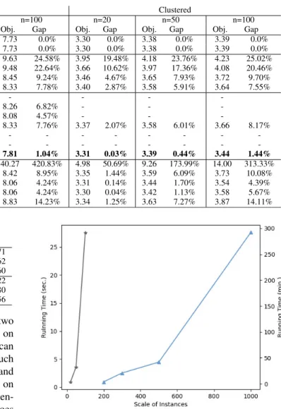
FIGURE 2. The running time of GNN-MCTS on different scale instances.
The gray polyline and blue polyline represent the running time of GNN-MCTS on small scale and larger scale instances, respectively. Best viewed in color.
32 instances in parallel. After 10 epochs, we report the time taken to solve each test instance (see Table4). Our method is slower than other learning-based methods due to the scouting exploration. Our code is written in Python and we notice that the speed of the MCTS procedure can be increased by coding it in C++. It is to be mentioned that the Gurobi solves the instances of TSP1000 very slowly and it could not give any feasible solution even after running for 10 hours.
Due to the GNN and MCTS, it is difficult to analyze the time complexity of the GNN-MCTS, so we visualize the running time of GNN-MCTS on instances of different sizes (see in Fig.2). By comparing the steepness of two polylines, we can conclude that the time complexity of GNN-MCTS is lower on larger scale instances.
Moreover, we analyze the running time of each part of the GNN-MCTS. Before deriving a tour, our method needs a large number of rollouts, where each rollout consists of four phases, which are selection, expansion, simulation and
TABLE 3. GNN-MCTS and other methods’ generalization on random instances.
TABLE 4. Running times of different methods.
TABLE 5. Running time of four phases in each rollouts.
backpropagation. The time cost of four phases in each rollout is shown in Table5. We can see that the simulation phase takes up almost all the time.
MCTS has been proven to converge to optimal solu- tions under assumptions of infinite memory and computation time (see [20] for more information). Compared with basic MCTS, GNN-MCTS replaces the uniform random selection strategy by a learned value function in simulation phase, i.e., incorporating specialized knowledge in MCTS, and the latter approach typically allows for faster convergence at the expense of simplicity and generality.
E. ABLATION STUDY 1) AVERAGE VS BEST
We analyze the effects of different strategies used in the GNN-MCTS procedure. The comparison of the two strate- gies are:
• Best. Unlike in AlphaGo, we track the best action value found under the subtree of each node for determining its exploitation value. At the end of several rollouts, we select the node with the best (biggest) action value as the next move in the root position.
• Average. As with the strategy used in AlphaGo, which is common in a two-player game, we track the average action value found under the subtree of each node as its exploitation value. Rather than selecting the node with the best (biggest) action value, we select the most visited node as the next move in the root position.
We use GNN-MCTS represents that tree search uses
‘‘Best’’ strategy and GNN-MCTSave. represents that tree search uses ‘‘Average’’ strategy. Table 1 shows the Gap between the solutions of our approach with two strategies and the best-known solution for TSP20, TSP50, and TSP100.
From the results of GNN-MCTS and GNN-MCTSave., we can see that the performance of our method is affected seriously when using the ‘‘Average’’ strategy. We believe that the performance of GNN-MCTSave. is degraded as the average action value under a node is not a good estimate if the optimal value under the node is surrounded by some inferior values.
2) COMPONENT CONTRIBUTION ANALYSIS OF GNN-MCTS We conduct a controlled experiment on the test set to ana- lyze the contribution of each component to the presented approach.
• Instead of the MCTS, we use SE-GNN to derive tours directly, i.e., to select the vertex with the largest prior probability at each step; we call this version as GNN-MCTS-t (without tree search).
• We replace the value function h(s) (see in Algorithm1) with random rollout function to evaluate the state during MCTS procedure; we call this version as GNN-MCTS-v (without value function).
• We take the output of the SE-GNN out of the picture and initialize prior probability to be 1 for newly expanded nodes; we call this version as GNN-MCTS-p (without prior probability provided by SE-GNN).
• A pure MCTS, which removes SE-GNN prior and replace value function h(s) with random rollout function, is listed for comparison; we call this version as MCTS (equal to GNN-MCTS-p,v).
Table 1 shows the Gap between the solution of each approach and the best-known solution for different TSP instances. As a whole, the performance (‘‘Gap’’ measure) of GNN-MCTS-t drops a lot from that of GNN-MCTS, which shows that the developed MCTS can efficiently prevent the algorithm from falling into any local optimum and it plays an important role in enhancing the performance of our method.
We make further detail analysis of the reasons why the algorithm is improved. Firstly, by comparing the perfor- mances of GNN-MCTS-p and GNN-MCTS, we can conclude that SE-GNN prior could help MCTS to effectively reduce
VOLUME 8, 2020 108425
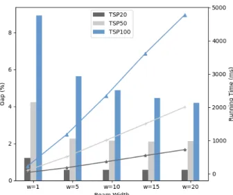
FIGURE 3. The performance of the value function with different beam width. Histogram represents ‘‘Gap’’ and polyline indicates running time.
Best viewed in color.
the search space so that MCTS can allocate more computing resources to the states with high action value. Secondly, the results obtained from GNN-MCTS-v and GNN-MCTS show that an appropriate value function h(s) can well estimate the tour length from the state of the leaf node to the final state, and it enables MCTS to perform better than that using just a random rollout function. Finally, by comparing the performances of GNN-MCTS-p, GNN-MCTS-v and other learning-based methods, we can see that when one compo- nent is removed from GNN-MCTS, i.e., SE-GNN prior or value function, our method can still derive a reasonable tour and perform well than other learning-based methods. That is, when it is difficult to design appropriate components for other similar problems, our method could achieve satisfactory results even with only one of them.
3) FURTHER ANALYSIS OF VALUE FUNCTION
We conduct experiments to explore the effects of different beam widths on the performance of the value function. Since the beam width mainly affects the performance of the value function, we use the result of this function as a measure and define the ‘‘Gap’’ as reported in Table1. Specifically, we set beam width to 1, 5, 10, 15, 20, and test the performance of the value function on random instances including TSP20, TSP50, and TSP100. We also count the time cost of the value func- tion when settings different beam widths. The experimental results are shown in Fig.3.
When the beam width is increased from 1 to 5, the performance of the value function is greatly improved.
However, as the beam width continues to increase, the improvement in the value function becomes less notice- able. Moreover, the running time of the value function increases about 5 times when the beam width is increased from 1 to 5. The above results show that we need to make a trade-off between the performance and the time cost of the value function.
4) COMPARISON WITH OTHER GRAPH NEURAL NETWORKS Compared with basic GNN [40] and GCN [50], [51], SE-GNN integrates edge information for computing new node feature, thus it should extract more information and perform well than basic GNN and GCN. To support this statement, we compare the performances of basic GNN, GCN, and SE-GNN on random instances, including TSP20, TSP50, and TSP100. We derive tours by directly using the neural network, i.e., selecting vertex with the largest prior probability at each step. The performance of the three GNN is reported in Table6.
The performances of the GNN, GCN, and SE-GNN show that edge features are important for the TSP. We agree that in principle the neural network should have learned the distance information from the coordinates of the vertices. It is a simple thing for people, but our empirical results indicate that it is difficult for the neural network to learn such distance information.
Moreover, we conduct a controlled experiment to ana- lyze why SE-GNN performs better than other GNNs. Com- pared with Crystal Graph Convolutional Neural Networks (CGCNN) [43] and Message Passing Neural Networks (MPNN) [42], the highest improvement of SE-GNN occurs as the single perceptron is replaced with a multilayer per- ceptron (MLP). To verify this point, we test the perfor- mance of SE-GNNσ which replaces MLP in (3) with a single perceptron (σ).
As shown in Table6, the performances of SE-GNNσ and CGCNN are comparable. However, when the single percep- tron is replaced with MLP, the performance of the SG-GNN is greatly improved, especially in the ‘‘Gap’’ metric. These results show that the MLP, which is used as a non-linear mapping function, plays an important role in achieving better performance.
In addition to different mapping functions, the edge fea- tures fusion mechanism of SE-GNN and other GNNs are also different. MPNN considers the edge features as a kind of metric to measure the usefulness of the neighbors of a node.
However, the SE-GNN and CGCNN consider edge features and node features to be equally important during the updating process. The results of SE-GNN, CGCNN and MPNN show that the integration mechanism used in SE-GNN and CGCNN is more suitable for the TSP.
5) DIFFERENT SETTINGS OF SE-GNN
The SE-GNN has T = 3 update layers, which is deep enough for a vertex to aggregate information associated with its neighboring vertices. Since the input graph is composed of vertices tagged with 9-dimensional features, the width of the first layer is H0 = 9. The width of the other layers is identical: Ht =128 for t = 1, 2.
The SE-GNN has a deep architecture that consists of several update layers. Therefore, as the model gets deeper with more layers, more information can be aggregated by the vertices. We train SE-GNN with different number of layers
TABLE 6. Performance of different neural networks on random instances.
TABLE 7. Effect of the number of layers on random instances.
on random instances including TSP20, TSP50, and TSP100.
We directly use the prior probability to derive a tour sequence, i.e., to select the vertex with the largest prior probability at each step.
The results in Table7 show that the performance of SE- GNN will become better as the number of network layers increases. However, three layers are enough for SE-GNN to extract features for the TSP in our experiments. Therefore, the three-layer SE-GNN is used by default.
V. CONCLUSION
In this work we tackle the classical traveling salesman prob- lem (TSP) by combining a graph neural network (GNN) and Monte Carlo Tree Search (MCTS). For better representation of the features of TSP, we train a developed GNN to integrate node features with edge features in a better way and to return the prior probability for each vertex as the deciding factor for the inclusion of the node to the partial tour. Instead of directly using the prior probability evaluated by GNN to derive a tour, we combine the GNN with the MCTS to provide a more reliable decision as the output of MCTS is the feedback information by fusing the prior probability with the scouting exploration. The experimental results show that the proposed approach can obtain shorter tours than other state-of-the-art learning-based methods. Also, the proposed approach has a good generalization capability on larger instances even if it is trained on smaller instances. We see the presented work as a step towards a family of solvers for NP-hard problems, which leverages both GNN and MCTS.
APPENDIX
EXTENSION TO TSP
To make the method of Li et al. [15] applicable to TSP, we make some changes as follows,
1) Li et al. adopt the hindsight loss and train GNN to generate multiple probability maps to differentiate mul- tiple optimal solutions for the same graph. However, the optimal tour is unique for TSP. So we modify their model by removing the hindsight loss and training GNN to output single probability map.
2) Li et al. propose a breadth-first tree search to increase the diversity of solutions, which maintains a queue of incomplete solutions and randomly chooses one of them to expand in each step. Li et al. also use graph reduction algorithms [52], [53] to reduce the search space, but such graph reduction algorithms are not available for TSP.
To reduce the search space, we only expand the states with top three prior probability output by GNN and then add these states to the queue.
ACKNOWLEDGMENT
The author Zhihao Xing thanks Kaixuan Zhao and Zhicheng Wang for the help in experiments by the existing methods:
Pointer Net and Dai et al.’s method, and also thanks Wenjing Huang, Qingsong Xie, Peiying Li, and Sicong Zang for help- ful discussions. The authors thank anonymous reviewers for all the comments and suggestions.
REFERENCES
[1] D. L. Applegate, R. E. Bixby, V. Chvatal, and W. J. Cook, The Trav- eling Salesman Problem: A Computational Study. Princeton, NJ, USA:
Princeton Univ. Press, 2006.
[2] C. H. Papadimitriou, ‘‘The Euclidean travelling salesman problem is NP- complete,’’ Theor. Comput. Sci., vol. 4, no. 3, pp. 237–244, Jun. 1977.
[3] E. L. Lawler, J. K. Lenstra, A. H. G. Rinnooy Kan, and D. B. Shmoys, ‘‘The traveling salesman problem: A guided tour of combinatorial optimization,’’
J. Oper. Res. Soc., vol. 37, no. 6, p. 655, Jun. 1986.
[4] M. T. Goodrich and R. Tamassia, ‘‘The christofides approximation algo- rithm,’’ Algorithm Design Application. Hoboken, NJ, USA: Wiley, 2015, pp. 513–514.
[5] D. S. Johnson and L. A. McGeoch, ‘‘The traveling salesman problem:
A case study in local optimization,’’ Local search Combinat. Optim., vol. 1, no. 1, pp. 215–310, 1997.
[6] M. Dorigo and L. M. Gambardella, ‘‘Ant colonies for the travelling sales- man problem,’’ Bio Syst., vol. 43, no. 2, p. 73, 1997.
[7] K. He, G. Gkioxari, P. Dollár, and R. Girshick, ‘‘Mask R-CNN,’’ in Proc.
IEEE Int. Conf. Comput. Vis., 2017, pp. 2961–2969.
[8] Y. LeCun, Y. Bengio, and G. Hinton, ‘‘Deep learning,’’ Nature, vol. 521, no. 7553, p. 436, 2015.
[9] O. Vinyals, M. Fortunato, and N. Jaitly, ‘‘Pointer networks,’’ in Proc. Int.
Conf. Neural Inf. Process. Syst., 2015 pp. 2692–2700.
[10] I. Bello, H. Pham, Q. V. Le, M. Norouzi, and S. Bengio, ‘‘Neural combi- natorial optimization with reinforcement learning,’’ in Proc. 5th Int. Conf.
Learn. Represent. (ICLR), Toulon, France, Apr. 2017, pp. 1–8.
[11] W. Kool, H. van Hoof, and M. Welling, ‘‘Attention, learn to solve routing problems!’’ in Proc. Int. Conf. Learn. Represent., 2019, pp. 1–8.
VOLUME 8, 2020 108427
[12] H. Dai, E. Khalil, Y. Zhang, B. Dilkina, and L. Song, ‘‘Learning combi- natorial optimization algorithms over graphs,’’ in Proc. Adv. Neural Inf.
Process. Syst., 2017, pp. 6348–6358.
[13] M. Prates, P. H. Avelar, H. Lemos, L. C. Lamb, and M. Y. Vardi, ‘‘Learning to solve np-complete problems: A graph neural network for decision TSP,’’
in Proc. AAAI Conf. Artif. Intell., vol. 33, 2019, pp. 4731–4738.
[14] E. Groshev, A. Tamar, M. Goldstein, S. Srivastava, and P. Abbeel, ‘‘Learn- ing generalized reactive policies using deep neural networks,’’ in Proc.
AAAI Spring Symp., 2018, pp. 1–5.
[15] Z. Li, Q. Chen, and V. Koltun, ‘‘Combinatorial optimization with graph convolutional networks and guided tree search,’’ in Proc. Adv. Neural Inf.
Process. Syst., 2018, pp. 539–548.
[16] M. Gasse, D. Chételat, N. Ferroni, L. Charlin, and A. Lodi, ‘‘Exact combi- natorial optimization with graph convolutional neural networks,’’ in Proc.
Adv. Neural Inf. Process. Syst., 2019, pp. 15554–15566.
[17] M. Deudon, P. Cournut, A. Lacoste, Y. Adulyasak, and L. M. Rousseau,
‘‘Learning heuristics for the TSP by policy gradient,’’ in Proc. Int. Conf.
Integr. Constraint Program., 2018, pp. 170–181.
[18] D. Silver, A. Huang, C. J. Maddison, A. Guez, L. Sifre, G. van den Driessche, J. Schrittwieser, I. Antonoglou, V. Panneershelvam, M. Lanctot, S. Dieleman, D. Grewe, J. Nham, N. Kalchbrenner, I. Sutskever, T. Lillicrap, M. Leach, K. Kavukcuoglu, T. Graepel, and D. Hassabis, ‘‘Mastering the game of go with deep neural networks and tree search,’’ Nature, vol. 529, no. 7587, pp. 484–489, Jan. 2016.
[19] R. Coulom, ‘‘Efficient selectivity and backup operators in monte-carlo tree search,’’ in Proc. Int. Conf. Comput. Games. Springer, 2006, pp. 72–83.
[20] L. Kocsis and C. Szepesvári, ‘‘Bandit based monte-carlo planning,’’ in Proc. Eur. Conf. Mach. Learn.Springer, 2006, pp. 282–293.
[21] L. Xu, ‘‘Deep bidirectional intelligence: AlphaZero, deep IA-search, deep IA-infer, and TPC causal learning,’’ Appl. Informat., vol. 5, no. 1, p. 5, Dec. 2018.
[22] L. Xu, ‘‘An overview and perspectives on bidirectional intelligence: Lmser duality, double IA harmony, and causal computation,’’ IEEE/CAA J.
Autom. Sinica, vol. 6, no. 4, pp. 865–893, Jul. 2019.
[23] L. Xu, ‘‘Deep ia-bi and five actions in circling,’’ in Intelligence Science and Big Data Engineering Visual Data Engineering, Z. Cui, J. Pan, S. Zhang, L. Xiao, and J. Yang, Eds. Cham, Switzerland: Springer, 2019, pp. 1–21.
[24] L. Xu, P. Yan, and T. Chang, ‘‘Algorithm cnneim—A and its mean com- plexity,’’ in Proc. 2nd Int. Conf. Comput. Appl. Beijing, China: IEEE Press, Jun. 1987, pp. 494–499.
[25] Z. Xing, S. Tu, and L. Xu, ‘‘Solve traveling salesman problem by Monte Carlo tree search and deep neural network,’’ 2020, arXiv:2005.06879.
[Online]. Available: http://arxiv.org/abs/2005.06879
[26] X. Gao, S. Tu, and L. Xu, ‘‘A∗ tree search for portfolio man- agement,’’ 2019, arXiv:1901.01855. [Online]. Available: http://arxiv.
org/abs/1901.01855
[27] J. J. Hopfield and D. W. Tank, ‘‘Neural computation of decisions in optimization problems,’’ Biol. Cybern., vol. 52, no. 3, p. 141, 1985.
[28] V. den Bout and Miller, ‘‘A traveling salesman objective function that works,’’ in Proc. IEEE Int. Conf. Neural Netw., Jul. 1988, pp. 299–303.
[29] Brandt, W. Yao, Laub, and Mitra, ‘‘Alternative networks for solving the traveling salesman problem and the list-matching problem,’’ in Proc. IEEE Int. Conf. Neural Netw., 1988, pp. 333–340.
[30] F. Favata and R. Walker, ‘‘A study of the application of kohonen-type neu- ral networks to the travelling salesman problem,’’ Biol. Cybern., vol. 64, no. 6, pp. 463–468, 1991.
[31] J. C. Fort, ‘‘Solving a combinatorial problem via self-organizing process:
An application of the kohonen algorithm to the traveling salesman prob- lem,’’ Biol. Cybern., vol. 59, no. 1, pp. 33–40, Jun. 1988.
[32] B. Angéniol, G. de La Croix Vaubois, and J.-Y. Le Texier, ‘‘Self-organizing feature maps and the travelling salesman problem,’’ Neural Netw., vol. 1, no. 4, pp. 289–293, Jan. 1988.
[33] T. Kohonen, ‘‘Self-organized formation of topologically correct feature maps,’’ Biol. Cybern., vol. 43, no. 1, pp. 59–69, 1982.
[34] D. Bahdanau, K. Cho, and Y. Bengio, ‘‘Neural machine translation by jointly learning to align and translate,’’ in 3rd Int. Conf. Learn. Represent., 2015, pp. 1–8.
[35] V. Mnih, A. P. Badia, M. Mirza, A. Graves, T. P. Lillicrap, T. Harley, D. Silver, and K. Kavukcuoglu, ‘‘Asynchronous methods for deep rein- forcement learning,’’ in Proc. 33nd Int. Conf. Mach. Learn., 2016, pp. 1928–1937.
[36] A. Vaswani, N. Shazeer, N. Parmar, J. Uszkoreit, L. Jones, A. N. Gomez, L. Kaiser, and I. Polosukhin, ‘‘Attention is all you need,’’ in Proc. Int. Conf.
Neural Inf. Process. Syst., 2017, pp. 5998–6008.
[37] H. Dai, B. Dai, and L. Song, ‘‘Discriminative embeddings of latent variable models for structured data,’’ in Proc. 33nd Int. Conf. Mach. Learn. (ICML), 2016, pp. 2702–2711.
[38] D. J. Rosenkrantz, R. E. Stearns, and P. M. Lewis, ‘‘An analysis of several heuristics for the traveling salesman problem,’’ in Proc. Fundam. Problems Comput., Essays Honor Professor Daniel J. Rosenkrantz, 2013, pp. 45–69.
[39] A. Nowak, S. Villar, A. S. Bandeira, and J. Bruna, ‘‘Revised note on learning algorithms for quadratic assignment with graph neural networks,’’ 2017, arXiv:1706.07450. [Online]. Available:
http://arxiv.org/abs/1706.07450
[40] W. Hamilton, Z. Ying, and J. Leskovec, ‘‘Inductive representation learn- ing on large graphs,’’ in Proc. Adv. Neural Inf. Process. Syst., 2017, pp. 1024–1034.
[41] C. D. Rosin, ‘‘Multi-armed bandits with episode context,’’ Ann. Math.
Artif. Intell., vol. 61, no. 3, pp. 203–230, Mar. 2011.
[42] J. Gilmer, S. S. Schoenholz, P. F. Riley, O. Vinyals, and G. E. Dahl, ‘‘Neural message passing for quantum chemistry,’’ in Proc. 34th Int. Conf. Mach.
Learn., vol. 70, 2017, pp. 1263–1272.
[43] T. Xie and J. C. Grossman, ‘‘Crystal graph convolutional neural networks for an accurate and interpretable prediction of material properties,’’ Phys.
Rev. Lett., vol. 120, no. 14, Apr. 2018, Art. no. 145301.
[44] K. Xu, W. Hu, J. Leskovec, and S. Jegelka, ‘‘How powerful are graph neural networks?’’ in Proc. Int. Conf. Learn. Represent., 2019, pp. 1–10.
[45] D. S. Johnson, G. Gutin, L. A. Mcgeoch, A. Yeo, W. Zhang, and A. Zverovitch, ‘‘Experimental analysis of heuristics for the ATSP,’’ in Proc.
Local Search Combinat. Optim., 2001, pp. 445–487.
[46] D. Applegate, R. Bixby, V. Chvatal, and W. Cook. (2006). Concorde TSP Solver. [Online]. Available: http://www.math.uwaterloo.ca/tsp/concorde/
[47] G. Optimization. (2013). Gurobi optimizer 5.0. [Online]. Available:
http://www.gurobi.com
[48] D. P. Kingma and J. Ba, ‘‘Adam: A method for stochastic opti- mization,’’ 2014, arXiv:1412.6980. [Online]. Available: http://arxiv.
org/abs/1412.6980
[49] R. S. Sutton and A. G. Barto, Reinforcement Learning: An Introduction.
Cambridge, MA, USA: MIT Press, 2018.
[50] M. Defferrard, X. Bresson, and P. Vandergheynst, ‘‘Convolutional neural networks on graphs with fast localized spectral filtering,’’ in Proc. Adv.
Neural Inf. Process. Syst., 2016, pp. 3844–3852.
[51] T. N. Kipf and M. Welling, ‘‘Semi-supervised classification with graph convolutional networks,’’ in Proc. 5th Int. Conf. Learn. Represent., 2017, pp. 1–8.
[52] T. Akiba and Y. Iwata, ‘‘Branch-and-reduce exponential/FPT algorithms in practice: A case study of vertex cover,’’ Theor. Comput. Sci., vol. 609, pp. 211–225, Jan. 2016.
[53] S. Lamm, P. Sanders, C. Schulz, D. Strash, and R. F. Werneck, ‘‘Finding near-optimal independent sets at scale,’’ J. Heuristics, vol. 23, no. 4, pp. 207–229, Aug. 2017.
ZHIHAO XING received the B.S. degree in software engineering from Shandong University, Jinan, China, in 2016. He is currently pursu- ing the M.Phil. degree in computer science and technology with Shanghai Jiao Tong University, Shanghai, China.
His research interests include machine learning and combinatorial optimization problems.
SHIKUI TU (Member, IEEE) received the B.Sc.
degree from Peking University, in 2006, and the Ph.D. degree from The Chinese University of Hong Kong, in 2012.
From December 2012 to January 2017, he was a Postdoctoral Associate with UMass, Worces- ter. He is currently a tenure-track Associate Professor with the Department of Computer Science and Engineering, Shanghai Jiao Tong University (SJTU). He is also the Academic Secretary with the Center for Cognitive Machines and Computational Health (CMaCH), SJTU. He has published more than 30 academic papers in top conferences and journals, including Science, Cell, NAR, and so on with high impact factors. His research interests include machine learning and bioinformatics.