Hardware and Software for

(1)

H.3 Scheduling and Structuring Code for Parallelism H-12 H.4 Hardware Support for Exposing Parallelism: Predicated Instructions H-23

H.5 Hardware Support for Compiler Speculation H-27

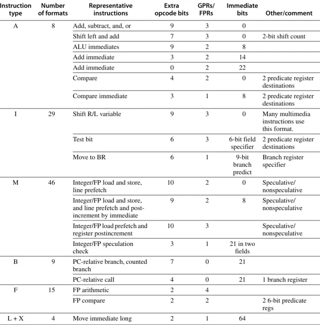
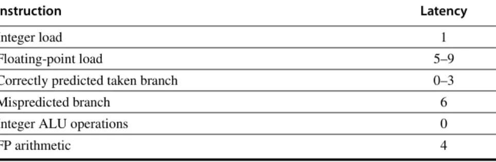
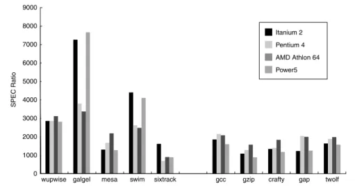
H.6 The Intel IA-64 Architecture and Itanium Processor H-32

H.7 Concluding Remarks H-43

(2)

H

Hardware and Software for

VLIW and EPIC

¹

The EPIC approach is based on the application of massive resources.

These resources include more load-store, computational, and branch units, as well as larger, lower-latency caches than would be required for a superscalar processor. Thus, IA-64 gambles that, in the future, power will not be the critical limitation, and that massive resources, along with the machinery to exploit them, will not penalize performance with their adverse effect on clock speed, path length, or CPI factors.

M. Hopkins in a commentary on the EPIC approach and the IA-64 architecture (2000)

(3)

In this chapter, we discuss compiler technology for increasing the amount of parallelism that we can exploit in a program as well as hardware support for these compiler techniques. The next section defines when a loop is parallel, how a dependence can prevent a loop from being parallel, and techniques for eliminating some types of dependences. The following section discusses the topic of scheduling code to improve parallelism. These two sections serve as an introduction to these techniques.

We do not attempt to explain the details of ILP-oriented compiler techniques, since that would take hundreds of pages, rather than the 20 we have allotted.

Instead, we view this material as providing general background that will enable the reader to have a basic understanding of the compiler techniques used to exploit ILP in modern computers.

Hardware support for these compiler techniques can greatly increase their effectiveness, and Sections H.4 and H.5 explore such support. The IA-64 repre- sents the culmination of the compiler and hardware ideas for exploiting parallelism statically and includes support for many of the concepts proposed by researchers during more than a decade of research into the area of compiler-based instruction-level parallelism. Section H.6 provides a description and performance analyses of the Intel IA-64 architecture and its second-generation implementa- tion, Itanium 2.

The core concepts that we exploit in statically based techniques—finding parallelism, reducing control and data dependences, and using speculation—are the same techniques we saw exploited in Chapter 3 using dynamic techniques. The key difference is that the techniques in this appendix are applied at compile time by the compiler, rather than at runtime by the hardware. The advantages of compile time techniques are primarily two: They do not burden runtime execution with any inefficiency, and they can take into account a wider range of the program than a runtime approach might be able to incorporate. As an example of the latter, the next section shows how a compiler might determine that an entire loop can be executed in parallel; hardware techniques might or might not be able to find such parallelism. The major disadvantage of static approaches is that they can use only compile time information. Without runtime information, compile time techniques must often be conservative and assume the worst case.

Loop-level parallelism is normally analyzed at the source level or close to it, while most analysis of ILP is done once instructions have been generated by the compiler. Loop-level analysis involves determining what dependences exist among the operands in a loop across the iterations of that loop. For now, we will

H.1 Introduction: Exploiting Instruction-Level Parallelism Statically

H.2 Detecting and Enhancing Loop-Level Parallelism

(4)

H.2 Detecting and Enhancing Loop-Level Parallelism ■ H-3

consider only data dependences, which arise when an operand is written at some point and read at a later point. Name dependences also exist and may be removed by renaming techniques like those we explored in Chapter 3.

The analysis of loop-level parallelism focuses on determining whether data accesses in later iterations are dependent on data values produced in earlier itera- tions; such a dependence is called a loop-carried dependence. Most of the exam- ples we considered in Section 3.2 have no loop-carried dependences and, thus, are loop-level parallel. To see that a loop is parallel, let us first look at the source representation:

for (i=1000; i>0; i=i–1) x[i] = x[i] + s;

In this loop, there is a dependence between the two uses of x[i], but this dependence is within a single iteration and is not loop carried. There is a dependence between successive uses of i in different iterations, which is loop carried, but this dependence involves an induction variable and can be easily recognized and eliminated. We saw examples of how to eliminate dependences involving induction variables during loop unrolling in Section 3.2, and we will look at additional examples later in this section.

Because finding loop-level parallelism involves recognizing structures such as loops, array references, and induction variable computations, the compiler can do this analysis more easily at or near the source level, as opposed to the machine-code level. Let’s look at a more complex example.

Example Consider a loop like this one:

for (i=1; i<=100; i=i+1) {

A[i+1] = A[i] + C[i]; /* S1 */

B[i+1] = B[i] + A[i+1]; /* S2 */

}

Assume that A, B, and C are distinct, nonoverlapping arrays. (In practice, the arrays may sometimes be the same or may overlap. Because the arrays may be passed as parameters to a procedure, which includes this loop, determining whether arrays overlap or are identical often requires sophisticated, interprocedural analysis of the program.) What are the data dependences among the statements S1 and S2 in the loop?

Answer There are two different dependences:

1. S1 uses a value computed by S1 in an earlier iteration, since iteration i com- putes A[i+1], which is read in iteration i+1. The same is true of S2 for B[i]

and B[i+1].

2. S2 uses the value, A[i+1], computed by S1 in the same iteration.

(5)

These two dependences are different and have different effects. To see how they differ, let’s assume that only one of these dependences exists at a time.

Because the dependence of statement S1 is on an earlier iteration of S1, this dependence is loop carried. This dependence forces successive iterations of this loop to execute in series.

The second dependence (S2 depending on S1) is within an iteration and is not loop carried. Thus, if this were the only dependence, multiple iterations of the loop could execute in parallel, as long as each pair of statements in an iteration were kept in order. We saw this type of dependence in an example in Section 3.2, where unrolling was able to expose the parallelism.

It is also possible to have a loop-carried dependence that does not prevent parallelism, as the next example shows.

Example Consider a loop like this one:

for (i=1; i<=100; i=i+1) {

A[i] = A[i] + B[i]; /* S1 */

B[i+1] = C[i] + D[i]; /* S2 */

}

What are the dependences between S1 and S2? Is this loop parallel? If not, show how to make it parallel.

Answer Statement S1 uses the value assigned in the previous iteration by statement S2, so there is a loop-carried dependence between S2 and S1. Despite this loop-carried dependence, this loop can be made parallel. Unlike the earlier loop, this dependence is not circular: Neither statement depends on itself, and, although S1 depends on S2, S2 does not depend on S1. A loop is parallel if it can be written without a cycle in the dependences, since the absence of a cycle means that the dependences give a partial ordering on the statements.

Although there are no circular dependences in the above loop, it must be transformed to conform to the partial ordering and expose the parallelism. Two observations are critical to this transformation:

1. There is no dependence from S1 to S2. If there were, then there would be a cycle in the dependences and the loop would not be parallel. Since this other dependence is absent, interchanging the two statements will not affect the execution of S2.

2. On the first iteration of the loop, statement S1 depends on the value of B[1]

computed prior to initiating the loop.

These two observations allow us to replace the loop above with the following code sequence:

(6)

A[1] = A[1] + B[1];

for (i=1; i<=99; i=i+1) { B[i+1] = C[i] + D[i];

A[i+1] = A[i+1] + B[i+1];

}

B[101] = C[100] + D[100];

The dependence between the two statements is no longer loop carried, so iterations of the loop may be overlapped, provided the statements in each iteration are kept in order.

Our analysis needs to begin by finding all loop-carried dependences. This dependence information is inexact, in the sense that it tells us that such a depen- dence may exist. Consider the following example:

for (i=1;i<=100;i=i+1) { A[i] = B[i] + C[i]

D[i] = A[i] * E[i]

}

The second reference to A in this example need not be translated to a load instruction, since we know that the value is computed and stored by the previous statement; hence, the second reference to A can simply be a reference to the register into which A was computed. Performing this optimization requires knowing that the two references are always to the same memory address and that there is no intervening access to the same location. Normally, data dependence analysis only tells that one reference may depend on another; a more complex analysis is required to determine that two references must be to the exact same address. In the example above, a simple version of this analysis suffices, since the two references are in the same basic block.

Often loop-carried dependences are in the form of a recurrence:

for (i=2;i<=100;i=i+1) { Y[i] = Y[i-1] + Y[i];

}

A recurrence is when a variable is defined based on the value of that variable in an earlier iteration, often the one immediately preceding, as in the above fragment. Detecting a recurrence can be important for two reasons: Some architectures (especially vector computers) have special support for executing recurrences, and some recurrences can be the source of a reasonable amount of parallelism. To see how the latter can be true, consider this loop:

for (i=6;i<=100;i=i+1) { Y[i] = Y[i-5] + Y[i];

}

(7)

On the iteration i, the loop references element i – 5. The loop is said to have a dependence distance of 5. Many loops with carried dependences have a depen- dence distance of 1. The larger the distance, the more potential parallelism can be obtained by unrolling the loop. For example, if we unroll the first loop, with a dependence distance of 1, successive statements are dependent on one another;

there is still some parallelism among the individual instructions, but not much. If we unroll the loop that has a dependence distance of 5, there is a sequence of five statements that have no dependences, and thus much more ILP. Although many loops with loop-carried dependences have a dependence distance of 1, cases with larger distances do arise, and the longer distance may well provide enough parallelism to keep a processor busy.

Finding Dependences

Finding the dependences in a program is an important part of three tasks: (1) good scheduling of code, (2) determining which loops might contain parallelism, and (3) eliminating name dependences. The complexity of dependence analysis arises because of the presence of arrays and pointers in languages like C or C++, or pass-by-reference parameter passing in FORTRAN. Since scalar variable references explicitly refer to a name, they can usually be analyzed quite easily, with aliasing because of pointers and reference parameters causing some complications and uncertainty in the analysis.

How does the compiler detect dependences in general? Nearly all dependence analysis algorithms work on the assumption that array indices are affine. In sim- plest terms, a one-dimensional array index is affine if it can be written in the form a × i + b, where a and b are constants and i is the loop index variable. The index of a multidimensional array is affine if the index in each dimension is affine.

Sparse array accesses, which typically have the form x[y[i]], are one of the major examples of nonaffine accesses.

Determining whether there is a dependence between two references to the same array in a loop is thus equivalent to determining whether two affine functions can have the same value for different indices between the bounds of the loop. For example, suppose we have stored to an array element with index value a× i + b and loaded from the same array with index value c × i + d, where i is the for-loop index variable that runs from m to n. A dependence exists if two condi- tions hold:

1. There are two iteration indices, j and k, both within the limits of the for loop.

That is, m ≤ j ≤ n, m ≤ k ≤ n.

2. The loop stores into an array element indexed by a × j + b and later fetches from that same array element when it is indexed by c × k + d. That is, a × j + b = c × k + d.

(8)

In general, we cannot determine whether a dependence exists at compile time. For example, the values of a, b, c, and d may not be known (they could be values in other arrays), making it impossible to tell if a dependence exists. In other cases, the dependence testing may be very expensive but decidable at compile time. For example, the accesses may depend on the iteration indices of multiple nested loops. Many programs, however, contain primarily simple indices where a, b, c, and d are all constants. For these cases, it is possible to devise rea- sonable compile time tests for dependence.

As an example, a simple and sufficient test for the absence of a dependence is the greatest common divisor (GCD) test. It is based on the observation that if a loop-carried dependence exists, then GCD (c,a) must divide (d – b). (Recall that an integer, x, divides another integer, y, if we get an integer quotient when we do the division y /x and there is no remainder.)

Example Use the GCD test to determine whether dependences exist in the following loop:

for (i=1; i<=100; i=i+1) { X[2*i+3] = X[2*i] * 5.0;

}

Answer Given the values a = 2, b = 3, c = 2, and d = 0, then GCD(a,c) = 2, and d – b = –3.

Since 2 does not divide –3, no dependence is possible.

The GCD test is sufficient to guarantee that no dependence exists; however, there are cases where the GCD test succeeds but no dependence exists. This can arise, for example, because the GCD test does not take the loop bounds into account.

In general, determining whether a dependence actually exists is NP complete.

In practice, however, many common cases can be analyzed precisely at low cost.

Recently, approaches using a hierarchy of exact tests increasing in generality and cost have been shown to be both accurate and efficient. (A test is exact if it precisely determines whether a dependence exists. Although the general case is NP complete, there exist exact tests for restricted situations that are much cheaper.)

In addition to detecting the presence of a dependence, a compiler wants to classify the type of dependence. This classification allows a compiler to recog- nize name dependences and eliminate them at compile time by renaming and copying.

Example The following loop has multiple types of dependences. Find all the true dependences, output dependences, and antidependences, and eliminate the output dependences and antidependences by renaming.

(9)

for (i=1; i<=100; i=i+1) { Y[i] = X[i] / c; /* S1 */

X[i] = X[i] + c; /* S2 */

Z[i] = Y[i] + c; /* S3 */

Y[i] = c - Y[i]; /* S4 */

}

Answer The following dependences exist among the four statements:

1. There are true dependences from S1 to S3 and from S1 to S4 because of Y[i]. These are not loop carried, so they do not prevent the loop from being considered parallel. These dependences will force S3 and S4 to wait for S1 to complete.

2. There is an antidependence from S1 to S2, based on X[i].

3. There is an antidependence from S3 to S4 for Y[i].

4. There is an output dependence from S1 to S4, based on Y[i].

The following version of the loop eliminates these false (or pseudo) dependences:

for (i=1; i<=100; i=i+1 {

/* Y renamed to T to remove output dependence */

T[i] = X[i] / c;

/* X renamed to X1 to remove antidependence */

X1[i] = X[i] + c;

/* Y renamed to T to remove antidependence */

Z[i] = T[i] + c;

Y[i] = c - T[i];

}

After the loop, the variable X has been renamed X1. In code that follows the loop, the compiler can simply replace the name X by X1. In this case, renaming does not require an actual copy operation but can be done by substituting names or by register allocation. In other cases, however, renaming will require copying.

Dependence analysis is a critical technology for exploiting parallelism. At the instruction level, it provides information needed to interchange memory references when scheduling, as well as to determine the benefits of unrolling a loop.

For detecting loop-level parallelism, dependence analysis is the basic tool. Effec- tively compiling programs to either vector computers or multiprocessors depends critically on this analysis. The major drawback of dependence analysis is that it applies only under a limited set of circumstances—namely, among references within a single loop nest and using affine index functions. Thus, there is a wide variety of situations in which array-oriented dependence analysis cannot tell us what we might want to know, including the following:

(10)

■ When objects are referenced via pointers rather than array indices (but see discussion below)

■ When array indexing is indirect through another array, which happens with many representations of sparse arrays

■ When a dependence may exist for some value of the inputs but does not exist in actuality when the code is run since the inputs never take on those values

■ When an optimization depends on knowing more than just the possibility of a dependence but needs to know on which write of a variable does a read of that variable depend

To deal with the issue of analyzing programs with pointers, another type of analysis, often called points-to analysis, is required (see Wilson and Lam [1995]).

The key question that we want answered from dependence analysis of pointers is whether two pointers can designate the same address. In the case of complex dynamic data structures, this problem is extremely difficult. For example, we may want to know whether two pointers can reference the same node in a list at a given point in a program, which in general is undecidable and in practice is extremely difficult to answer. We may, however, be able to answer a simpler question: Can two pointers designate nodes in the same list, even if they may be separate nodes? This more restricted analysis can still be quite useful in scheduling memory accesses performed through pointers.

The basic approach used in points-to analysis relies on information from three major sources:

1. Type information, which restricts what a pointer can point to.

2. Information derived when an object is allocated or when the address of an object is taken, which can be used to restrict what a pointer can point to. For example, if p always points to an object allocated in a given source line and q never points to that object, then p and q can never point to the same object.

3. Information derived from pointer assignments. For example, if p may be assigned the value of q, then p may point to anything q points to.

There are several cases where analyzing pointers has been successfully applied and is extremely useful:

■ When pointers are used to pass the address of an object as a parameter, it is possible to use points-to analysis to determine the possible set of objects referenced by a pointer. One important use is to determine if two pointer parameters may designate the same object.

■ When a pointer can point to one of several types, it is sometimes possible to determine the type of the data object that a pointer designates at different parts of the program.

■ It is often possible to separate out pointers that may only point to a local object versus a global one.

(11)

There are two different types of limitations that affect our ability to do accurate dependence analysis for large programs. The first type of limitation arises from restrictions in the analysis algorithms. Often, we are limited by the lack of applica- bility of the analysis rather than a shortcoming in dependence analysis per se. For example, dependence analysis for pointers is essentially impossible for programs that use pointers in arbitrary fashion—such as by doing arithmetic on pointers.

The second limitation is the need to analyze behavior across procedure boundaries to get accurate information. For example, if a procedure accepts two parameters that are pointers, determining whether the values could be the same requires analyzing across procedure boundaries. This type of analysis, called interprocedural analysis, is much more difficult and complex than analysis within a single procedure. Unlike the case of analyzing array indices within a single loop nest, points-to analysis usually requires an interprocedural analysis. The reason for this is simple. Suppose we are analyzing a program segment with two pointers; if the analysis does not know anything about the two pointers at the start of the program segment, it must be conservative and assume the worst case. The worst case is that the two pointers may designate the same object, but they are not guaranteed to designate the same object. This worst case is likely to propagate through the analysis, producing useless information. In practice, getting fully accurate interprocedural information is usually too expensive for real programs.

Instead, compilers usually use approximations in interprocedural analysis. The result is that the information may be too inaccurate to be useful.

Modern programming languages that use strong typing, such as Java, make the analysis of dependences easier. At the same time the extensive use of proce- dures to structure programs, as well as abstract data types, makes the analysis more difficult. Nonetheless, we expect that continued advances in analysis algorithms, combined with the increasing importance of pointer dependency analysis, will mean that there is continued progress on this important problem.

Eliminating Dependent Computations

Compilers can reduce the impact of dependent computations so as to achieve more instruction-level parallelism (ILP). The key technique is to eliminate or reduce a dependent computation by back substitution, which increases the amount of parallelism and sometimes increases the amount of computation required. These techniques can be applied both within a basic block and within loops, and we describe them differently.

Within a basic block, algebraic simplifications of expressions and an optimi- zation called copy propagation, which eliminates operations that copy values, can be used to simplify sequences like the following:

DADDUI R1,R2,#4 DADDUI R1,R1,#4

(12)

to

DADDUI R1,R2,#8

assuming this is the only use of R1. In fact, the techniques we used to reduce multiple increments of array indices during loop unrolling and to move the increments across memory addresses in Section 3.2 are examples of this type of optimization.

In these examples, computations are actually eliminated, but it is also possible that we may want to increase the parallelism of the code, possibly even increasing the number of operations. Such optimizations are called tree height reduction because they reduce the height of the tree structure representing a com- putation, making it wider but shorter. Consider the following code sequence:

ADD R1,R2,R3

ADD R4,R1,R6

ADD R8,R4,R7

Notice that this sequence requires at least three execution cycles, since all the instructions depend on the immediate predecessor. By taking advantage of associativity, we can transform the code and rewrite it as

ADD R1,R2,R3

ADD R4,R6,R7

ADD R8,R1,R4

This sequence can be computed in two execution cycles. When loop unrolling is used, opportunities for these types of optimizations occur frequently.

Although arithmetic with unlimited range and precision is associative, com- puter arithmetic is not associative, for either integer arithmetic, because of limited range, or floating-point arithmetic, because of both range and precision.

Thus, using these restructuring techniques can sometimes lead to erroneous behavior, although such occurrences are rare. For this reason, most compilers require that optimizations that rely on associativity be explicitly enabled.

When loops are unrolled, this sort of algebraic optimization is important to reduce the impact of dependences arising from recurrences. Recurrences are expressions whose value on one iteration is given by a function that depends on the previous iterations. When a loop with a recurrence is unrolled, we may be able to algebraically optimize the unrolled loop, so that the recurrence need only be evaluated once per unrolled iteration. One common type of recurrence arises from an explicit program statement, such as:

sum = sum + x;

(13)

Assume we unroll a loop with this recurrence five times. If we let the value of x on these five iterations be given by x1, x2, x3, x4, and x5, then we can write the value of sum at the end of each unroll as:

sum = sum + x1 + x2 + x3 + x4 + x5;

If unoptimized, this expression requires five dependent operations, but it can be rewritten as:

sum = ((sum + x1) + (x2 + x3)) + (x4 + x5);

which can be evaluated in only three dependent operations.

Recurrences also arise from implicit calculations, such as those associated with array indexing. Each array index translates to an address that is computed based on the loop index variable. Again, with unrolling and algebraic optimization, the dependent computations can be minimized.

We have already seen that one compiler technique, loop unrolling, is useful to uncover parallelism among instructions by creating longer sequences of straight- line code. There are two other important techniques that have been developed for this purpose: software pipelining and trace scheduling.

Software Pipelining: Symbolic Loop Unrolling

Software pipelining is a technique for reorganizing loops such that each itera- tion in the software-pipelined code is made from instructions chosen from different iterations of the original loop. This approach is most easily understood by looking at the scheduled code for the unrolled loop, which appeared in the example on page 78. The scheduler in this example essentially interleaves instructions from different loop iterations, so as to separate the dependent instructions that occur within a single loop iteration. By choosing instructions from different iterations, dependent computations are separated from one another by an entire loop body, increasing the possibility that the unrolled loop can be scheduled without stalls.

A software-pipelined loop interleaves instructions from different iterations without unrolling the loop, as illustrated in Figure H.1. This technique is the software counterpart to what Tomasulo’s algorithm does in hardware. The software- pipelined loop for the earlier example would contain one load, one add, and one store, each from a different iteration. There is also some start-up code that is needed before the loop begins as well as code to finish up after the loop is com- pleted. We will ignore these in this discussion, for simplicity.

H.3 Scheduling and Structuring Code for Parallelism

(14)

H.3 Scheduling and Structuring Code for Parallelism ■ H-13

Example Show a software-pipelined version of this loop, which increments all the ele- ments of an array whose starting address is in R1 by the contents of F2:

Loop: L.D F0,0(R1)

ADD.D F4,F0,F2

S.D F4,0(R1)

DADDUI R1,R1,#-8

BNE R1,R2,Loop

You may omit the start-up and clean-up code.

Answer Software pipelining symbolically unrolls the loop and then selects instructions from each iteration. Since the unrolling is symbolic, the loop overhead instructions (the DADDUI and BNE) need not be replicated. Here’s the body of the unrolled loop without overhead instructions, highlighting the instructions taken from each iteration:

Iteration i: L.D F0,0(R1)

ADD.D F4,F0,F2 S.D F4,0(R1) Iteration i+1: L.D F0,0(R1) ADD.D F4,F0,F2

S.D F4,0(R1)

Iteration i+2: L.D F0,0(R1) ADD.D F4,F0,F2 S.D F4,0(R1)

Figure H.1 A software-pipelined loop chooses instructions from different loop iter- ations, thus separating the dependent instructions within one iteration of the origi- nal loop. The start-up and finish-up code will correspond to the portions above and below the software-pipelined iteration.

Software- pipelined iteration

Iteration

0 Iteration

1 Iteration

2 Iteration

3 Iteration

4

(15)

The selected instructions from different iterations are then put together in the loop with the loop control instructions:

Loop: S.D F4,16(R1) ;stores into M[i]

ADD.D F4,F0,F2 ;adds to M[i-1]

L.D F0,0(R1) ;loads M[i-2]

DADDUI R1,R1,#-8

BNE R1,R2,Loop

This loop can be run at a rate of 5 cycles per result, ignoring the start-up and clean-up portions, and assuming that DADDUI is scheduled before the ADD.D and that the L.D instruction, with an adjusted offset, is placed in the branch delay slot.

Because the load and store are separated by offsets of 16 (two iterations), the loop should run for two fewer iterations. Notice that the reuse of registers (e.g., F4, F0, and R1) requires the hardware to avoid the write after read (WAR) hazards that would occur in the loop. This hazard should not be a problem in this case, since no data-dependent stalls should occur.

By looking at the unrolled version we can see what the start-up code and finish-up code will need to be. For start-up, we will need to execute any instructions that correspond to iteration 1 and 2 that will not be executed. These instructions are the L.D for iterations 1 and 2 and the ADD.D for iteration 1. For the finish-up code, we need to execute any instructions that will not be executed in the final two iterations. These include the ADD.D for the last iteration and the S.D for the last two iterations.

Register management in software-pipelined loops can be tricky. The previous example is not too hard since the registers that are written on one loop iteration are read on the next. In other cases, we may need to increase the number of iterations between when we issue an instruction and when the result is used. This increase is required when there are a small number of instructions in the loop body and the latencies are large. In such cases, a combination of software pipelining and loop unrolling is needed.

Software pipelining can be thought of as symbolic loop unrolling. Indeed, some of the algorithms for software pipelining use loop-unrolling algorithms to figure out how to software-pipeline the loop. The major advantage of software pipelining over straight loop unrolling is that software pipelining consumes less code space. Software pipelining and loop unrolling, in addition to yielding a bet- ter scheduled inner loop, each reduce a different type of overhead. Loop unrolling reduces the overhead of the loop—the branch and counter update code.

Software pipelining reduces the time when the loop is not running at peak speed to once per loop at the beginning and end. If we unroll a loop that does 100 iterations a constant number of times, say, 4, we pay the overhead 100/4 = 25 times—every time the inner unrolled loop is initiated. Figure H.2 shows this behavior graphically. Because these techniques attack two different types of overhead, the best performance can come from doing both. In practice, compila-

(16)

tion using software pipelining is quite difficult for several reasons: Many loops require significant transformation before they can be software pipelined, the trade-offs in terms of overhead versus efficiency of the software-pipelined loop are complex, and the issue of register management creates additional complexi- ties. To help deal with the last two of these issues, the IA-64 added extensive hardware sport for software pipelining. Although this hardware can make it more efficient to apply software pipelining, it does not eliminate the need for complex compiler support, or the need to make difficult decisions about the best way to compile a loop.

Global Code Scheduling

In Section 3.2 we examined the use of loop unrolling and code scheduling to improve ILP. The techniques in Section 3.2 work well when the loop body is straight-line code, since the resulting unrolled loop looks like a single basic block.

Similarly, software pipelining works well when the body is a single basic block, since it is easier to find the repeatable schedule. When the body of an unrolled loop contains internal control flow, however, scheduling the code is much more complex. In general, effective scheduling of a loop body with internal control flow will require moving instructions across branches, which is global code scheduling.

In this section, we first examine the challenge and limitations of global code Figure H.2 The execution pattern for (a) a software-pipelined loop and (b) an unrolled loop. The shaded areas are the times when the loop is not running with maxi- mum overlap or parallelism among instructions. This occurs once at the beginning and once at the end for the software-pipelined loop. For the unrolled loop it occurs m/n times if the loop has a total of m iterations and is unrolled n times. Each block repre- sents an unroll of n iterations. Increasing the number of unrollings will reduce the start- up and clean-up overhead. The overhead of one iteration overlaps with the overhead of the next, thereby reducing the impact. The total area under the polygonal region in each case will be the same, since the total number of operations is just the execution rate multiplied by the time.

(a) Software pipelining

Proportional to number of unrolls

Overlap between unrolled iterations

Time Wind-down code Start-up

code

(b) Loop unrolling

Time Number

of overlapped operations

Number of overlapped operations

(17)

scheduling. In Section H.4 we examine hardware support for eliminating control flow within an inner loop, then we examine two compiler techniques that can be used when eliminating the control flow is not a viable approach.

Global code scheduling aims to compact a code fragment with internal control structure into the shortest possible sequence that preserves the data and control dependences. The data dependences force a partial order on operations, while the control dependences dictate instructions across which code cannot be easily moved. Data dependences are overcome by unrolling and, in the case of memory operations, using dependence analysis to determine if two references refer to the same address. Finding the shortest possible sequence for a piece of code means finding the shortest sequence for the critical path, which is the longest sequence of dependent instructions.

Control dependences arising from loop branches are reduced by unrolling.

Global code scheduling can reduce the effect of control dependences arising from conditional nonloop branches by moving code. Since moving code across branches will often affect the frequency of execution of such code, effectively using global code motion requires estimates of the relative frequency of different paths. Although global code motion cannot guarantee faster code, if the frequency information is accurate, the compiler can determine whether such code movement is likely to lead to faster code.

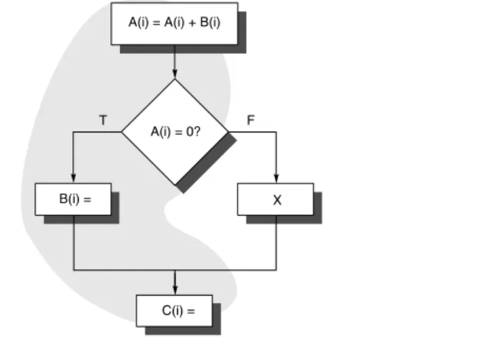
Global code motion is important since many inner loops contain conditional statements. Figure H.3 shows a typical code fragment, which may be thought of as an iteration of an unrolled loop, and highlights the more common control flow.

Figure H.3 A code fragment and the common path shaded with gray. Moving the assignments to B or C requires a more complex analysis than for straight-line code. In this section we focus on scheduling this code segment efficiently without hardware assistance. Predication or conditional instructions, which we discuss in the next section, provide another way to schedule this code.

A(i) = A(i) + B(i)

T F

B(i) = X

A(i) = 0?

C(i) =

(18)

Effectively scheduling this code could require that we move the assignments to B and C to earlier in the execution sequence, before the test of A. Such global code motion must satisfy a set of constraints to be legal. In addition, the movement of the code associated with B, unlike that associated with C, is speculative: It will speed the computation up only when the path containing the code would be taken.

To perform the movement of B, we must ensure that neither the data flow nor the exception behavior is changed. Compilers avoid changing the exception behavior by not moving certain classes of instructions, such as memory references, that can cause exceptions. In Section H.5, we will see how hardware support allows for more opportunities for speculative code motion and removes control dependences. Although such enhanced support for speculation can make it possible to explore more opportunities, the difficulty of choosing how to best compile the code remains complex.

How can the compiler ensure that the assignments to B and C can be moved without affecting the data flow? To see what’s involved, let’s look at a typical code generation sequence for the flowchart in Figure H.3. Assuming that the addresses for A, B, C are in R1, R2, and R3, respectively, here is such a sequence:

LD R4,0(R1) ;load A

LD R5,0(R2) ;load B

DADDU R4,R4,R5 ;Add to A

SD R4,0(R1) ;Store A

...

BNEZ R4,elsepart ;Test A

... ;then part

SD ...,0(R2) ;Stores to B

...

J join ;jump over else

elsepart: ... ;else part

X ;code for X

...

join: ... ;after if

SD ...,0(R3) ;store C[i]

Let’s first consider the problem of moving the assignment to B to before the BNEZ instruction. Call the last instruction to assign to B before the if statement i.

If B is referenced before it is assigned either in code segment X or after the if statement, call the referencing instruction j. If there is such an instruction j, then moving the assignment to B will change the data flow of the program. In particu- lar, moving the assignment to B will cause j to become data dependent on the moved version of the assignment to B rather than on i, on which j originally depended. You could imagine more clever schemes to allow B to be moved even when the value is used: For example, in the first case, we could make a shadow copy of B before the if statement and use that shadow copy in X. Such schemes are usually avoided, both because they are complex to implement and because

(19)

they will slow down the program if the trace selected is not optimal and the operations end up requiring additional instructions to execute.

Moving the assignment to C up to before the first branch requires two steps.

First, the assignment is moved over the join point of the else part into the portion corresponding to the then part. This movement makes the instructions for C control dependent on the branch and means that they will not execute if the else path, which is the infrequent path, is chosen. Hence, instructions that were data dependent on the assignment to C, and which execute after this code fragment, will be affected. To ensure the correct value is computed for such instructions, a copy is made of the instructions that compute and assign to C on the else path. Second, we can move C from the then part of the branch across the branch condition, if it does not affect any data flow into the branch condition. If C is moved to before the if test, the copy of C in the else branch can usually be eliminated, since it will be redundant.

We can see from this example that global code scheduling is subject to many constraints. This observation is what led designers to provide hardware support to make such code motion easier, and Sections H.4 and H.5 explores such support in detail.

Global code scheduling also requires complex trade-offs to make code motion decisions. For example, assuming that the assignment to B can be moved before the conditional branch (possibly with some compensation code on the alternative branch), will this movement make the code run faster? The answer is, possibly! Similarly, moving the copies of C into the if and else branches makes the code initially bigger! Only if the compiler can successfully move the computation across the if test will there be a likely benefit.

Consider the factors that the compiler would have to consider in moving the computation and assignment of B:

■ What are the relative execution frequencies of the then case and the else case in the branch? If the then case is much more frequent, the code motion may be beneficial. If not, it is less likely, although not impossible, to consider moving the code.

■ What is the cost of executing the computation and assignment to B above the branch? It may be that there are a number of empty instruction issue slots in the code above the branch and that the instructions for B can be placed into these slots that would otherwise go empty. This opportunity makes the computation of B “free” at least to first order.

■ How will the movement of B change the execution time for the then case? If B is at the start of the critical path for the then case, moving it may be highly beneficial.

■ Is B the best code fragment that can be moved above the branch? How does it compare with moving C or other statements within the then case?

■ What is the cost of the compensation code that may be necessary for the else case? How effectively can this code be scheduled, and what is its impact on execution time?

(20)

As we can see from this partial list, global code scheduling is an extremely complex problem. The trade-offs depend on many factors, and individual decisions to globally schedule instructions are highly interdependent. Even choosing which instructions to start considering as candidates for global code motion is complex!

To try to simplify this process, several different methods for global code scheduling have been developed. The two methods we briefly explore here rely on a simple principle: Focus the attention of the compiler on a straight-line code segment representing what is estimated to be the most frequently executed code path. Unrolling is used to generate the straight-line code, but, of course, the complexity arises in how conditional branches are handled. In both cases, they are effectively straightened by choosing and scheduling the most frequent path.

Trace Scheduling: Focusing on the Critical Path

Trace scheduling is useful for processors with a large number of issues per clock, where conditional or predicated execution (see Section H.4) is inappropriate or unsupported, and where simple loop unrolling may not be sufficient by itself to uncover enough ILP to keep the processor busy. Trace scheduling is a way to organize the global code motion process, so as to simplify the code scheduling by incurring the costs of possible code motion on the less frequent paths. Because it can generate significant overheads on the designated infrequent path, it is best used where profile information indicates significant differences in frequency between different paths and where the profile information is highly indicative of program behavior independent of the input. Of course, this limits its effective applicability to certain classes of programs.

There are two steps to trace scheduling. The first step, called trace selection, tries to find a likely sequence of basic blocks whose operations will be put together into a smaller number of instructions; this sequence is called a trace.

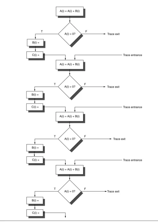
Loop unrolling is used to generate long traces, since loop branches are taken with high probability. Additionally, by using static branch prediction, other conditional branches are also chosen as taken or not taken, so that the resultant trace is a straight-line sequence resulting from concatenating many basic blocks. If, for example, the program fragment shown in Figure H.3 corresponds to an inner loop with the highlighted path being much more frequent, and the loop were unwound four times, the primary trace would consist of four copies of the shaded portion of the program, as shown in Figure H.4.

Once a trace is selected, the second process, called trace compaction, tries to squeeze the trace into a small number of wide instructions. Trace compaction is code scheduling; hence, it attempts to move operations as early as it can in a sequence (trace), packing the operations into as few wide instructions (or issue packets) as possible.

The advantage of the trace scheduling approach is that it simplifies the decisions concerning global code motion. In particular, branches are viewed as jumps into or out of the selected trace, which is assumed to be the most probable path.

(21)

Figure H.4 This trace is obtained by assuming that the program fragment in Figure H.3 is the inner loop and unwinding it four times, treating the shaded portion in Figure H.3 as the likely path. The trace exits correspond to jumps off the frequent path, and the trace entrances correspond to returns to the trace.

A(i) = A(i) + B(i)

T F

B(i) =

A(i) = 0?

C(i) =

Trace entrance

A(i) = A(i) + B(i)

T F

B(i) =

A(i) = 0?

C(i) =

Trace exit Trace exit

Trace entrance

A(i) = A(i) + B(i)

T F

B(i) =

A(i) = 0?

C(i) =

Trace exit

Trace entrance

A(i) = A(i) + B(i)

T F

B(i) =

C(i) =

A(i) = 0? Trace exit

(22)

When code is moved across such trace entry and exit points, additional bookkeeping code will often be needed on the entry or exit point. The key assumption is that the trace is so much more probable than the alternatives that the cost of the bookkeeping code need not be a deciding factor: If an instruction can be moved and thereby make the main trace execute faster, it is moved.

Although trace scheduling has been successfully applied to scientific code with its intensive loops and accurate profile data, it remains unclear whether this approach is suitable for programs that are less simply characterized and less loop intensive. In such programs, the significant overheads of compensation code may make trace scheduling an unattractive approach, or, at best, its effective use will be extremely complex for the compiler.

Superblocks

One of the major drawbacks of trace scheduling is that the entries and exits into the middle of the trace cause significant complications, requiring the compiler to generate and track the compensation code and often making it difficult to assess the cost of such code. Superblocks are formed by a process similar to that used for traces, but are a form of extended basic blocks, which are restricted to a single entry point but allow multiple exits.

Because superblocks have only a single entry point, compacting a superblock is easier than compacting a trace since only code motion across an exit need be considered. In our earlier example, we would form superblocks that contained only one entrance; hence, moving C would be easier. Furthermore, in loops that have a single loop exit based on a count (for example, a for loop with no loop exit other than the loop termination condition), the resulting superblocks have only one exit as well as one entrance. Such blocks can then be scheduled more easily.

How can a superblock with only one entrance be constructed? The answer is to use tail duplication to create a separate block that corresponds to the portion of the trace after the entry. In our previous example, each unrolling of the loop would create an exit from the superblock to a residual loop that handles the remaining iterations. Figure H.5 shows the superblock structure if the code fragment from Figure H.3 is treated as the body of an inner loop and unrolled four times. The residual loop handles any iterations that occur if the superblock is exited, which, in turn, occurs when the unpredicted path is selected. If the expected frequency of the residual loop were still high, a superblock could be created for that loop as well.

The superblock approach reduces the complexity of bookkeeping and scheduling versus the more general trace generation approach but may enlarge code size more than a trace-based approach. Like trace scheduling, superblock scheduling may be most appropriate when other techniques (e.g., if conversion) fail.

Even in such cases, assessing the cost of code duplication may limit the useful- ness of the approach and will certainly complicate the compilation process.

(23)

Loop unrolling, software pipelining, trace scheduling, and superblock scheduling all aim at trying to increase the amount of ILP that can be exploited by a processor issuing more than one instruction on every clock cycle. The Figure H.5 This superblock results from unrolling the code in Figure H.3 four times and creating a superblock.

C(i) = A(i) = A(i) + B(i)

T F

B(i) =

A(i) = 0?

C(i) =

A(i) = A(i) + B(i)

T F

B(i) =

A(i) = 0?

C(i) =

A(i) = A(i) + B(i)

T F

B(i) =

A(i) = 0?

C(i) =

A(i) = A(i) + B(i)

T F

B(i) =

A(i) = 0?

A(i) = A(i) + B(i)

T F

B(i) = X

A(i) = 0?

C(i) =

Execute n times Superblock exit

with n = 4

Superblock exit with n = 3

(24)

H.4 Hardware Support for Exposing Parallelism: Predicated Instructions ■ H-23

effectiveness of each of these techniques and their suitability for various archi- tectural approaches are among the hottest topics being actively pursued by researchers and designers of high-speed processors.

Techniques such as loop unrolling, software pipelining, and trace scheduling can be used to increase the amount of parallelism available when the behavior of branches is fairly predictable at compile time. When the behavior of branches is not well known, compiler techniques alone may not be able to uncover much ILP.

In such cases, the control dependences may severely limit the amount of parallelism that can be exploited. To overcome these problems, an architect can extend the instruction set to include conditional or predicated instructions. Such instruc- tions can be used to eliminate branches, converting a control dependence into a data dependence and potentially improving performance. Such approaches are useful with either the hardware-intensive schemes in Chapter 3 or the software- intensive approaches discussed in this appendix, since in both cases predication can be used to eliminate branches.

The concept behind conditional instructions is quite simple: An instruction refers to a condition, which is evaluated as part of the instruction execution. If the condition is true, the instruction is executed normally; if the condition is false, the execution continues as if the instruction were a no-op. Many newer architectures include some form of conditional instructions. The most common example of such an instruction is conditional move, which moves a value from one register to another if the condition is true. Such an instruction can be used to completely eliminate a branch in simple code sequences.

Example Consider the following code:

if (A==0) {S=T;}

Assuming that registers R1, R2, and R3 hold the values of A, S, and T, respectively, show the code for this statement with the branch and with the conditional move.

Answer The straightforward code using a branch for this statement is (remember that we are assuming normal rather than delayed branches)

BNEZ R1,L ADDU R2,R3,R0 L:

Using a conditional move that performs the move only if the third operand is equal to zero, we can implement this statement in one instruction:

CMOVZ R2,R3,R1

H.4 Hardware Support for Exposing Parallelism:

Predicated Instructions

(25)

The conditional instruction allows us to convert the control dependence present in the branch-based code sequence to a data dependence. ( This transformation is also used for vector computers, where it is called if conversion.) For a pipelined processor, this moves the place where the dependence must be resolved from near the front of the pipeline, where it is resolved for branches, to the end of the pipeline, where the register write occurs.

One obvious use for conditional move is to implement the absolute value function: A = abs (B), which is implemented as if (B<0) {A=-B;} else {A=B;}.

This if statement can be implemented as a pair of conditional moves, or as one unconditional move (A=B) and one conditional move (A=-B).

In the example above or in the compilation of absolute value, conditional moves are used to change a control dependence into a data dependence. This enables us to eliminate the branch and possibly improve the pipeline behavior. As issue rates increase, designers are faced with one of two choices: execute multiple branches per clock cycle or find a method to eliminate branches to avoid this requirement. Handling multiple branches per clock is complex, since one branch must be control dependent on the other. The difficulty of accurately predicting two branch outcomes, updating the prediction tables, and executing the correct sequence has so far caused most designers to avoid processors that execute multiple branches per clock. Conditional moves and predicated instructions provide a way of reducing the branch pressure. In addition, a conditional move can often eliminate a branch that is hard to predict, increasing the potential gain.

Conditional moves are the simplest form of conditional or predicated instructions and, although useful for short sequences, have limitations. In particular, using conditional move to eliminate branches that guard the execution of large blocks of code can be inefficient, since many conditional moves may need to be introduced.

To remedy the inefficiency of using conditional moves, some architectures support full predication, whereby the execution of all instructions is controlled by a predicate. When the predicate is false, the instruction becomes a no-op. Full predication allows us to simply convert large blocks of code that are branch dependent. For example, an if-then-else statement within a loop can be entirely converted to predicated execution, so that the code in the then case executes only if the value of the condition is true and the code in the else case executes only if the value of the condition is false. Predication is particularly valuable with global code scheduling, since it can eliminate nonloop branches, which significantly complicate instruction scheduling.

Predicated instructions can also be used to speculatively move an instruction that is time critical, but may cause an exception if moved before a guarding branch. Although it is possible to do this with conditional move, it is more costly.