行政院國家科學委員會專題研究計畫 成果報告
短產品生命週期需求模式下供應鏈協合規劃之研究(第 2 年)
研究成果報告(完整版)
計 畫 類 別 : 個別型
計 畫 編 號 : NSC 96-2416-H-011-007-MY2
執 行 期 間 : 97 年 08 月 01 日至 98 年 07 月 31 日 執 行 單 位 : 國立臺灣科技大學工業管理系
計 畫 主 持 人 : 周碩彥
計畫參與人員: 碩士班研究生-兼任助理人員:黃文宏 碩士班研究生-兼任助理人員:許馨尹 碩士班研究生-兼任助理人員:江御彰
報 告 附 件 : 出席國際會議研究心得報告及發表論文
處 理 方 式 : 本計畫可公開查詢
中 華 民 國 98 年 12 月 20 日
Inventory Management for Dependent Demand Characterized by Fractional Brownian Motion
Shu-Ting Yang
a, Shuo-Yan Chou
aa
Department of Industrial Management
National Taiwan University of Science and Technology
Abstract
Inventory management is an important issue in manufacturing. The goal in developing these inventory models is to determine the optimal order quantity and gain the maximum profit. Hence, in this thesis, we assume that the demand in the manufacture is under fractional Brownian motion. We also use fractional Brownian motion by the Hurst exponent in the fixed lead-time demand to modify (Q, r) inventory model. Finally, we simulated the fBm process by different H values for the lead time demand to develop an inventory policy. We compare the result with an independent model so that we could find out that our model is better than the assumed independent model. We hope that these results could provide managers to make a correct decision.
Keywords: fractional Brownian motion; Hurst exponent; (Q, r) inventory model
1. Introduction
Inventory management plays an important role in industry. In a company, if there are too many in stock or out-of-stock, there will be an increase in costs. Sometimes there would even be a loss in sales. As a result, we should have better inventory control and management techniques to order our products.
However, in order to have better inventory control, predicting demand is becoming more important. Sometimes the lead time demand is assumed to be independent of history. But we think the demand should be dependent to each other.
In addition, we have also found in literature that when the demand was uncertain, they usually assumed different probability density functions to model the lead time demand. But in 1958, Scarf addressed the newsboy problem where only the mean and the variance of the demand are known without any further assumptions about the form of the distribution of the demand [8].
In the previous research discoveries since 1956, Hurst discovered that a large time
series data of natural events seem to be governed by a simple relation and they are not
always independent to each other. He invented a new statistic theory, the rescaled
range analysis, to explain the “persistence” and “anti-persistence” of several natural
phenomena and finally obtained a Hurst exponent H, which measures the intensity of
long-range dependence in a time series. After Hurst’s findings, Mandelbrot put
forward a new theory, namely “fractional Brownian motion (fBm).” Fractional
Brownian motion is used to model the variation of many natural phenomena because
it considers the dependence between each increment. In regard to the above, we
consider that many situations where the variety of lead time demand exhibits some
shortage costs and the lead-time demand is under fractional Brownian motion have not been explored. Therefore, this thesis focuses on developing an inventory system with backorders and a fixed replenishment lead time demand influenced by the Hurst exponent. The objective is to minimize the total annual cost and to find out the optimal order quantity for managers to take appropriate inventory strategies.
2. Theoretical Background
2.1. The Hurst Phenomenon and Hurst law
Hurst (1956) [9] spent a lifetime inventing a new statistical method - the rescaled range analysis, also called R/S analysis or Hurst method. He solved the problems related to water storage by observing the discharge record from the Great Lakes of the Nile Basin in Egypt. He wanted to design an ideal reservoir that never overflows or empties. An ideal reservoir would store water from good years for use in bad ones. Also it necessitated a reservoir to be of sufficient capacity to meet the shortages that might occur during a century.
Hurst investigated the reservoir size that would be required to maintain the maximum possible steady discharge during the period from the lake. First, he calculated the mean discharge for the period n and the capacity of the reservoir as obtained by adding all the departures from the mean to form a series of accumulated totals. After that, in this series the difference can be found between the highest and lowest of these accumulated totals—that is, the range R . This range R is the storage that maintains the average discharge. According to this concept, Hurst proposed the rescaled range analysis.
Let there be a given year, t , such that a reservoir is fed by the discharge of water
average inflow is
1
1 [ (1) (2) ( )]
1 ( )
T
T
t
X X X X T
T T
X t
This average should equal the volume released per year from the reservoir. Then denote X t T
( , )as the accumulated departure of the influx X t
( )from the mean X :
T1
( , ) [( (1) ) ( (2) ) ( ( ) )]
[ ( ) ]
T T T
T
T t
X t T X X X X X t X
X t X
Let R
Tbe the difference between the minimum and the maximum accumulated inflow X contained in the reservoir over a period of T years. The explicit expression for R
Tis
1 1
max ( , ) min ( , )
T t T t T
R X t T X t T
And sample standard deviation S
Tis
2 2 2
1 [( (1) ) ( (2) ) ( ( ) ) ]
T T T T
S X X X X X T X
T
What Hurst discovered is that a large number of natural phenomena events called
Hurst phenomena, such as flood levels on the Nile, river discharges, global
temperature changes, mud sediments, and tree rings, seem to obey by a simple
relation with the rescaled range. It was be defined by the dimensionless ratio R S .
T THe sets R S
T T( aT )
H, namely Hurst Law, where H is coefficient called the Hurst
exponent. To compute H for each time series, he found that there are a lot of
records in times revealing that the rescales range, R S , is described very well by
T Twhere a
1/ 2, and then computes H for each time series (Wallis, 1970) [28] by
log( / )log( / 2)
T T
H R S
T
Hurst applied this rescaled range analysis to explain several natural phenomena with “persistence” or “anti-persistence”. Also, the Hurst exponent H can measure the intensity of long-range dependence in a time series. It provides information about the memory range or long correlations versus short correlations of time series processes.
There are many evidences in many different research fields that show the Hurst exponent mainly differs from 0.5, especially in many natural processes, like sunspot fluctuation, river discharges and rainfall levels. They also present a long-term
“memory effect” in processes, and all of them have values of H not equal to 0.5. Hurst devised an experiment that takes into account these kinds of natural processes that
“remember” earlier events. For instance, the river’s discharge depends not only on the current level of rainfall but also on earlier rainfall
(Mandelbrot and Wallis, 1969a;1969) [17] [18]. There are lots of statistical results collected by Hurst showing that for
many natural phenomena with H
0.5[9]. Also the process in fractional FourierTransformation or on the wavelet spectrum is said to have long range dependence, especially when
0.5 H
1 (Stoev et al., 2005) [26]. In addition, many real worldprocesses give H about 0.73. Especially, exacting self-similarity processes have H equals to 1.
Here we provide a summary of those analyses. They show that the Hurst exponent
provides three given information from 0 to 1:
(2) For
0.5 H
1, the Hurst phenomenon is the process displaying persistence on all time scales. In the rainfall levels case, if we had a decrease in the past, then we would see a decrease in the future—on the average. Consequently, an increasing trend in the past implies an increasing trend in the future for all processes. Thus, the process is positive dependence to each other.
(3) Moreover, if
0 H
0.5, the process has an anti-persistence behavior. There is a negative dependence between the increments. In other words, X t
( )will probably decrease/increase for t
t
0if it increased/decreased for t
0 0 .
2.2. The Fractional Brownian
motionWe mention that the most perfect crystal has many impurities and other defects that is placed at random. Randomness is inherent in all natural phenomena. Before, the study of random functions, namely Markov processes, people have been overwhelmingly devoted to sequences of independent random variables. Besides the empirical findings of the design of water system by Hurst and Hurst’s law, there is a common basic feature of many phenomena, namely the “span of interdependence”.
Mandelbrot and Van Ness (1968) proposed to designate a family of random functions, called fractional Brownian motion (fBm)
[19]. They believe that fBm does provideuseful models for a host of natural time series and therefore wish to present their properties of interest to scientists, engineers and statisticians.
The fractional Brownian motion (fBm) is a Gaussian process whose covariance
function is a generalization of Wiener process. Comparable with the classical
Brownian motion as seen in Appendix A given the value at X t , where ( )
1t
1t
2,
behavior over time. It is clear that there is a need for a version of the random process that has some memory of the past. Such a process was fBm introduced and analyzed by Mandelbrot and Van Ness (1968) [3]. It is defined by parameter H with
0 H
1. For H
0.5, the definition of a fractional Brownian motion reduces to that of classical Brownian motion. Crownover (1995)
[4] and Feder (1988) [7] also provedthat the H parameter of fBm is the Hurst exponent and the fBm satisfied the rescaled range analysis.
The following is a fractional Brownian motion defined by Falconer (1990) [6],
DefinitionA real stochastic process X t
( ), with t
[0, ), is a fractional Brownian motion with parameter H, called the Hurst exponent, where
0 H
1, such that
(1) X
(0)
0(2) X t
( )is almost surely continuous everywhere for t
[0, )(3) The increments have Gaussian increment property
2 1
( ) ( )
X X t X t
with mean zero and variance
2(t
2 t
1)2H, where t
2 t
1and is a positive constant.
A fractional Brownian motion with parameter H
0.5is the same as an ordinary Brownian motion.
Variance Law and Stationarity
Restating the variance part of the property gives us the variance law for
t
Ht t
X t
X (
2) (
1)]
2 2 1 2var[
for any t and
1t in the interval [a, b]. Since the variance depends only on the
2difference in t and
1t , not on the values themselves, the increments are stationary.
2Or Hsieh (1997) [9].
H H
s C t
X s t X
E [ (
)
( )]
2 2 [ ( 1) ( )]2C
H E X t X t , where s
1 Non-independence of IncrementsIn contrast with the ordinary Brownian motion, which satisfies the independent increments property, a fractional Brownian motion with parameter H
0.5does not satisfy this property.
Non-Markovian Behavior
If H
0.5, then X t
( ) X
(0)and X x h
(
)X t
( )tend to have the same sign, and X t
( )tends to be increasing in the future if it was increasing in the past. If
0.5
H , then X t
( ) X
(0)and X x h
(
)X t
( )tend to have opposite signs, and
( )X t trends to reverse. Combining these observations, it shows that a fractional Brownian motion is not a Markov process, except when H
0.5.
Statistical Self-similarity
The increments of a fractional Brownian motion satisfy
( ) ( ) 1H ( ( ) ( ))X t t X t X t r t X t
r
for any r
0. (The symbol means that the two random variables have same
such as coastlines, are statistically self-similarity. Parts of them show the same statistical properties at many scales. In other words, the whole object has the same shape as one or more of the parts.
Long range dependence
Most of the features of fractional Brownian motion are long range dependence; in the other hand, in particular, past increments are correlated with future increments.
Denote symbol B
H( ) t as fractional Brownian motion. We consider the relation between the increment of past B
H(0)
B
H(
t ) from time –t to 0 and the increment of future B
H( ) t
B
H(0) ; the correlation function of future increments B
H( ) t with past increments
B
H(
t ) may be written as:
2 1
2
[ ( ) ( )]
( ) 2 1
[ ( ) ]
H H H
H
E B t B t
C t E B t
Table 1
The variation of Hurst exponent
H
0.1 0.2 0.3 0.4 0.5 0.6 0.7 0.8 0.9
( )
C t -0.426 -0.340 -0.242 -0.129 0.000 0.149 0.320 0.516 0.741
Table 1 shows that when
H
0.5, C t
( )
0. That is, the increment in the past is uncorrelated with the increment in the future. It is the random process that has independent increments. However, when H
0.5, it is a random process of dependent increments. When an fBm with a Hurst exponent has
0.5 H
1,
( ) 0
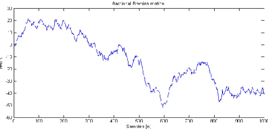
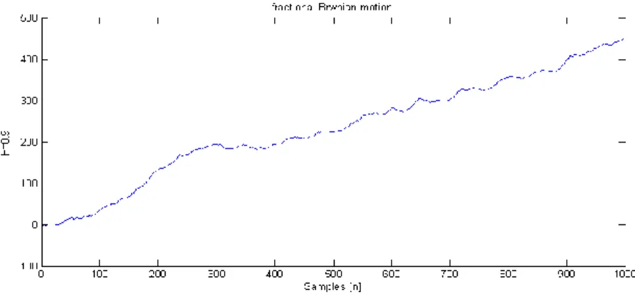
C t , the increments in the past and in the future have positive correlation. Its increments have a higher probability to increase or decrease while the preceding one is increasing or decreasing. We could say the process is persistent or there is trend-reinforcing behavior in the time series. It is a long-term memory. On the
increased or decreased in the past, then it will probably decrease or increase in the
future. The behaviors are illustrated in
Fig 1. For 0 H
0.5, the trend in the
amplitude of vibration is apparently greater; otherwise, the graph in
0.5 H
1is
not very rugged looking.
Fig. 1. Graphs of fractional Brownian motion starting at 0 for H=0.2, 0.3, 0.4, 0.6, 0.7,
0.8, and 0.9.
Fig. 1. Graphs of fractional Brownian motion starting at 0 for H=0.2, 0.3, 0.4, 0.6, 0.7, 0.8, and 0.9 (Cont.).
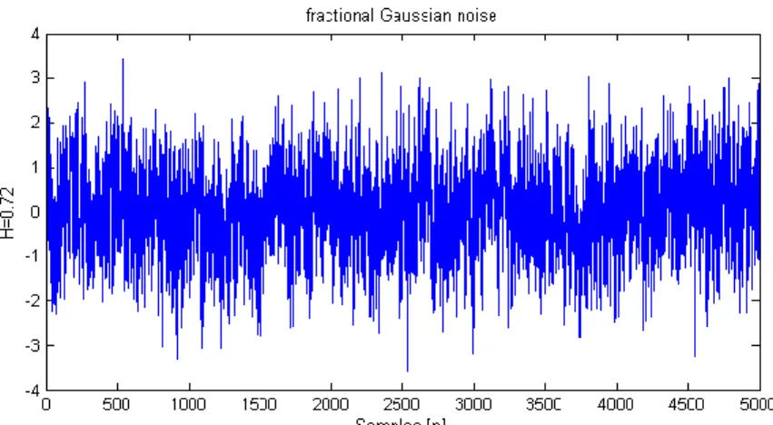
2.3. The fractional Gaussian noise
Fractional Gaussian noise (fGn) is derived from fractional Brownian motion (fBm) which is a long-range dependent Gaussian process with a Hurst parameter H and with stationary increments. In practice, the fBm plays a fundamental role in modeling long-range dependence and its increments that are used in modeling. The increment process of the fBm is fGn, which is expressed as
( , ) ( ) ( )
BH H H
X t B t B t
is a normal distribution with mean zero and variance
H2
2Hfor all t
[0, )and
[0, )
, where
H2is a position constant and
is the sampling period.
If H
0.5, the increments of an fBm are stationary. However, it depends on
random variables. Particularly, it is not short-term memory, but the long-term memory
that is affected most by the latest increments. The autocorrelation of fGn could be
seen in Magre and Guglielmi (1997) [19]. Fig 2 shows examples of fGn with a sample
size of 5000.
Fig. 2. An example of fGn with pre-determined Hurst parameter of 0.72
2.4. The dimension of the graph
Mandelbrot’s fractal geometry both provides a description and a mathematical model for many seemingly complex forms of those found in nature
[3]. Shapes suchas coastlines, mountains and clouds are not easily described by traditional Euclidean geometry. Further, they often possess a remarkable simplifying invariance under changes of magnification. In nature, this statistical self-similarity is the essential quality of fractals. It may be quantified by a fractal dimension, which is a number that agrees with our intuitive notion of dimension but need not to be an integer.
One of the main concepts of fractal geometry is the property of self-similarity. A D-dimensional self-similar object can be divided into N smaller copies of itself each of which is scaled down by a factor r ,
r
DN
1
For instance, one line replaced by 4 parts and the ratio is 1/3, and the curve will be
shown in
Fig 3 In this example, the dimension isD
1.26. It could be easily seen
that the fractal dimension is not an integer and is unlike the Euclidean dimension.
Fig. 3. The Koch Curve of N = 4 and r = 1/3 [3]
When D increases from 1 to 2, the resulting “curves” will progress from being
“line-like” to “filling” much of the plane. Hence, the fractal dimension D provides a quantitative measure of wig lines of the curves.
A one-variable fractional Brownian motion for the box dimension of the graph of a sample path can be calculated in the same way as that for an ordinary Brownian motion [3]. The Hurst exponent is also directly related to the fractal dimension, which gives a measure of the roughness of a surface. The relationship between the fractal dimension, D, and the Hurst exponent, H, is D
2 H .
3. Dependent Demand Pattern
3.1. Data research
Predicting the market demand is an important issue in product management.
Especially, in capacity planning where decision maker must depend on some of the data’s prediction to set up a schedule or make a procedure to meet what is needed.
Traditionally, many researches were done on the basis of normal distribution to
develop a measure of the economic model because the real probability density
sometimes have a dependent relation with the past ones.
Fractional Brownian motion was initially used in modeling hydrological phenomena. It also has been shown that fBm can be suitable for the analysis of computer network traffic. In the twentieth century, it was used in various fields as financial mathematics and random landscape generation. Moreover, the Hurst exponent, H, is a measure of the bias in Fractional Brownian motion. It is referred to as the “index of dependence” and the relative tendency of a time series to either cluster in a direction or strongly regress to the mean. Further, H parameter is a measure of the level of self-similarity of a time series that exhibits long-range dependence. H takes on values from 0.5 to 1. The closer H is to 1, the greater is the degree of persistence or long-rang dependence. With
0 H
0.5it implies an anti-persistent time series or mean-reverting processes. When H
0.5, it is Brownian motion.
In our research, we believe that the demand in the manufacture exists in a
dependent relation to its history and the demands are under the Fractional Brownian
motion. In other words, the demands of the manufacturing industry have the basic
feature of fBm that is the span of interdependence between their increments. In order
to verify our point, we collected some manufacturing data for monthly sales from the
Department of Statistics, Ministry of Economic Affairs, R.O.C. The data collected
was from 2000 to 2009. According to these actual monthly sales data in the market,
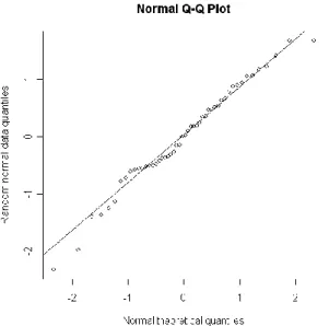
we accept them as our time series data. First, due to fBm being a Gaussian process,
we use Q-Q plot (see Appendix B) and the chi-square goodness-of-fit test (see
Appendix C) to test if our data is of normal distribution. If they do not conform, we
result, we could make a summarization. If H
0.5, we could say that the demands in the manufacture industry obey fBm.
Table 2 shows that our time series data information including the name of product,
the data collection period, the quantity collected, and the product’s origin.
Table 2 Research data
product data collection period quantity of data
sock ( 1000 dozen) 2000/1~2008/12 108
clock ( unit) 2000/12~2009/3 100
diesel fuel( kiloliters) 2000/12~2009/3 100
Source from Ministry of Economic Affairs
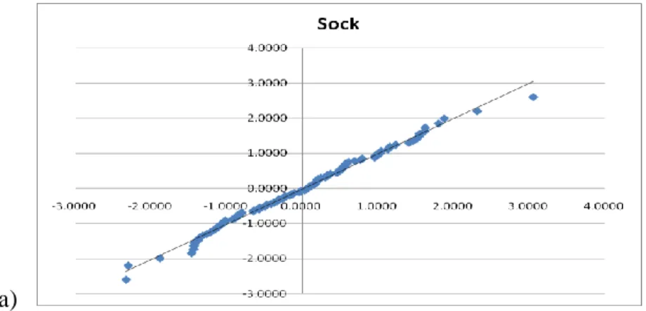
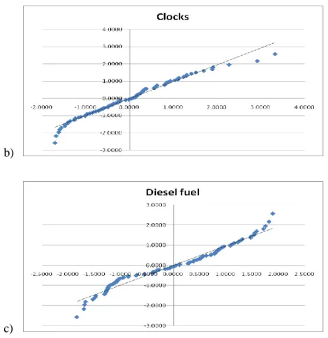
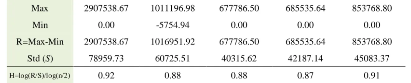
As revealed by
Fig 4, the Q-Q plots of three product data provide someinformation. We could see if the data have gathered near or almost close to the trendline, it could be a normal distribution.
a)
b)
c)
Fig. 4. Q-Q plot for twenty products
After plotting the Q-Q plot, we made a chi-square goodness-of-fit test to test if our data is also of normal distribution.
Table 3 illustrates one of three examples thatprocess the chi-square goodness-of-fit test. Compared with the significance level , that is desired to 0.05 now, if the value of the hypothesis test is larger than , we will reject the null hypotheses. As we would hope, the chi-square test does not reject the normality hypothesis for the normal distribution data set and does reject it for the non-normal cases.
Table 3
Chi-square goodness-of-fit test of (b) sock Let n is the sample size,
o is observed frequencies
ie is expected frequencies
i2 2 2
{ | 9.487}
0.05,5 1
C
Monthly Sales
(period)
Volume( o ) Probability(
ip )
ie
i n p
i (o
i e
i)2 (o
i e
i) /2e
ilow 850 9 0.092 9.914 0.836 0.084
850~1050 21 0.183 19.710 1.664 0.084
1050~1300 38 0.347 37.519 0.231 0.006
1300~1550 28 0.267 28.847 0.717 0.025
over 1550 12 0.111 12.010 0.000 0.000
sum 108 1.000 0.2
2 2
1
( )
0.2 9.5
k
k k
i k
o e
e C
2 2.05,4:
0.2 9.5 .
, .
the result of test
cannot reject
So the monthly sales of sock is normal distribution
Moreover,
Table 4 contains all of our remaining final products. It also providesdetails of the result including two important parameters, Hurst exponent H estimation by R/S analysis and fractional dimension D computation.
Table 4
Research data with Hurst exponent
Product Mean Range (R) Std Hurst (H) Fractional
Dimension (D)
(a) sock (1000 dozen) 1215.09 5075.52 273.66 0.73 1.27
(b) clock 174435.83 2907538.67 78959.73 0.92 1.08
(c) diesel fuel
( kiloliters) 1100469.22 11422180.58 283705.43 0.95 1.05
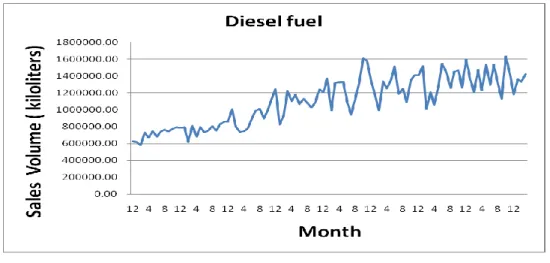
We also could see in
Table 5 when we calculate the Hurst exponent in differentshort period between 2000/12 to 2009/3, all values of H are close to the origin
0.92
H . We could infer that our data has a self-similar property.
Table 5
Hurst exponent of (b) clock data in different period
Max 2907538.67 1011196.98 677786.50 685535.64 853768.80
Min 0.00 -5754.94 0.00 0.00 0.00
R=Max-Min 2907538.67 1016951.92 677786.50 685535.64 853768.80 Std (S) 78959.73 60725.51 40315.62 42187.14 45083.37
H=log(R/S)/log(n/2) 0.92 0.88 0.88 0.87 0.91
Finally, we plot the time series data from monthly sales volume in Fig 5.
(a) Sock with H=0.73
(b) Clock with H=0.92
Fig. 5. Plot data sets for monthly sales in the market
(c) Diesel fuel with H=0.95
Fig. 5. Plot data sets for monthly sales in the market (Cont.)
3.2. Analysis result
According to Fig 5, we can see figures decay or growth happening slowly. Data
are not decreasing or increasing as rapidly at different times as in exponential decay.
These data show that they are not in short-range dependence but exist rather in long-range dependence.
As Table 4 shows, we observe that all H values are larger than 0.5. It proves our initial doubt that the demand of manufacturing is not following random walk. There appears to be persistent persistence and long-rang dependence. Mandelbrot supposes these are under fractional Brownian motion, not random work processes. An fBm is described as a series having long-term memory effects that when the former value is large, the latter will usually follow to be large. This relationship will break when exogenous events happen. It also verifies what Apley and Tsung discussed in 2002;
these cases with the Hurst exponent smaller than 0.5 are not discussed because the
fBm exhibited negative autocorrelation, a situation uncommon in industry
[1].shaking such as in (a) sock.
In our conclusion, we analyze that demands are belonging to the fBm in the manufacture of the item. So, describing market demand by using fBm is better and more suitable than using tradition statistical methods.
4. Inventory model
4.1. Introduction
Depending upon different demand process assumptions, inventory control model can be broadly separated into two types, deterministic and probabilistic models. In the probabilistic model, assumptions about the probability density function of the demand process are usually made. Various probability density functions have been applied to model demands for establishing inventory management policy.
Every probability density function has its own advantages and disadvantages for application in its field. In most situations, when we only know the mean and variance of demand in the process but do not know what the real probability density function in the demand process is; we would assume the probability density function is a normal distribution for the inventory model. But Scarf in 1958
[18]addressed the newsboy problem where the mean and the variance of the demand are the only known variables without any further assumptions about the form of the distribution of the demand. He also had expressed a closed form for the maximization profile and the optimal order quantity.
If we use a traditional inventory model, we think there will be a higher total cost
because we usually assume the demand to be independent. Many publications
assumed normality and independence in the inventory model. And there are others
independence by Bagchi et al. (1982) [2], Kottas and Lau (1970, 1980) [13] [17], Lau and Wang (1986)
[18], Ray (1980, 1989) [22] [23], and Van Ness and Stevenson(1983) [27]. In practice, demands show a tendency to be autocorrelated.
As we mentioned before, the demands in the manufacturing industry follow fractional Brownian motion. After Mandelbrot and Ness’s reporting, fBm has been used in different fields like hydrology, economics, astronomy, electronics, geophysics, finance and so forth. Many scientists, engineers and statisticians have used fBm to re-model their existing phenomena and problems. However, fBm is not used in inventory, quality control and other fields.
Moreover, Hurst proposed an ideal reservoir based upon the given record of observed discharges from the Great Lake of the Nile Basin; this whole idea is a suitable application in inventory management. For instance, the lead time demands are like the discharges of the river and the market is like the Nile lake. How much product should we make in order to meet the demand? The capacity management plays an important role in manufacturing. And our objective is to achieve fewer stocks and to gain maximum profit.
In order to reach our goal, we should construct our inventory model by fractional Brownian motion. Now we consider a fixed replenishment lead time, (Q, r) inventory model with known mean and variance. Then we use fBm to describe the lead time demand process and try to find a different solution.
4.2. Notations and assumptions
The notations below will be used in this thesis.
HC yearly per unit inventory holding cost UC unit cost
SC shortage cost VC variable cost
x unit time demand during lead time
t average value of x
tt fixed replenishment lead time H Hurst exponent,
0 H
1C
Ha positive constant from fractional Brownian motion X demand during the lead time t
iq allowable stockout probability during the lead time t
i ( )B r the expected shortage at the end of the period cycle N present stock at reorder point
fraction of the demand backordered during the stockout period ,
0,1 fixed penalty cost per unit stockout
0marginal profit (i.e., cost of lost demand) per unit Decision variables
Q order quantity r reorder point k safety factor
In order to clearly define the scope of the model, the following assumptions are made.
(1) The demand of fixed lead time X is composed of a sequence of demands x .
t0.5
H
1. When H
0.5, x is a random variable with a normal
tdistribution.
(3) We assume each item has the same fixed replenishment lead time. On the other hand, all t are the same.
(4) In original EOQ model, it is not permitted to be stockout. But we broke the assumption for pressing close to truth in this research. The symbol q represents the allowable stockout probability during t and the symbol presents the fraction of the fixed lead-time demand backordered during the stockout period.
So
1- is the ratio of the lost sales from the stockout.
(5) k is the safety factor where k statisfies P X
( r
)q and q represents the allowable stockout probability during t. Additionally, the safety stock equals the safety factor k multiplied by the standard deviation of the lead time demand. So the reorder point r is the expected demand during a fixed lead time plus the safety stock.
(6) As
0.5 H
1there exits “persistence”, that is, an increasing or decreasing trend in the past implies an increasing or decreasing trend in the future for all processes. When
0 H
0.5, we have “anti-persistence”. In these situations an increase or decrease in the past implies a decrease or increase in the future. For process with H
0.5, it becomes a common normal distribution demand inventory model.
4.3. Continuous-review System
In this inventory model, t is assumed to be the time lag and the fixed
demand of fixed replenishment lead time X is composed of a sequence of demands x , we divide by a fixed replenishment lead time
tt . We could get the average fixed lead-time demand t . According to fractional Brownian motion, the mean and variance of the fixed lead time demand X are t and C t
H 2 H.
When the fixed lead time demand X equals the reorder point r , the stock will satisfy demand. The shortage would not happen since X
r . But if, X
r a shortage would occur and then the expected inventory shortage
X r
X r prob X
at the end of period cycle is given by B r
( ). For
(0
1)the fraction of the backordered demand during the stockout period, the expected number of backorders per cycle is B r
( )and the expected demand lost sales per cycle is thus
(1
) ( )B r . Hence, the expected shortage cost per period cycle [
(1 )
o] ( ) B r is composed of the expected penalty cost B r
( )and the expected profit loss
o(1
) ( ) B r .
The expected net inventory levels that can be derived (Ravindran et al., 1987) [21]
immediately before and after the order Q arrives are r t
(1
) ( )B r and
(1 ) ( )Q r t B r respectively. Consequently, the average inventory on hand is
(1 ) ( )2
Q r t B r (1)
According to fractional Brownian motion r X k t k C t
H H, we have
(1 ) ( ) 2
H H
Q k C t B r (2)
The expected annual cost function in this model formulation is identified to four
separate cost components by unit cost (UC), reordering cost (RC), holding cost (HC)
=UC× Q (3)
Reordering cost component: reorder cost (RC) × number of orders places (1)
= RC (4)
Holding cost component: An average stock of (
(1 ) ( ) 2H H
Q k C t B r )
held for a time period
= HC× (
(1 ) ( )2
H H
Q k C t B r ) × T (5)
Shortage cost component: an expected shortage of
x r
x r prob x
held
for a time period
= SC ×
x r
x r prob x
=[
o(1
)] ( ) B r (6)
Adding these four components together, we can get the expected approximate annual total cost per cycle:
( , )
[ (1 ) ( )] [ (1 ) ] ( )
2
H
H o
EAC Q k UC RC HC SC
UC Q RC HC T Q k C t B r B r
(7) Then dividing by T and substituting Q D T gives the total cost per unit time:
( , )
[ (1 ) ( )]
[ (1 ) ] ( )
2
H H
o
UC RC HC SC
EAC Q k
T T T T
HC T Q k C t B r
B r
UC Q RC
(8) Because the unit cost component is fixed and not influenced by the order quantity, we can only concentrate on the other terms which form the variable cost (VC) with fractional Brownian motion. That is:
( , ) [ (1 ) ( )] [ (1 ) ] ( )
2
H
H o
D Q D
VC Q k RC HC k C t B r B r
Q Q
(9) We want to find the order quantity that maximizes the expected profit against the worst possible distribution of the demand with knowing only the mean and variance of the lead time demand. So we consider any cumulative distribution, which is called G, of the lead time demand. We let
denote the class of G’s cumulative density functions with finite mean t and variance C
Ht
2H.
Since the distribution G of X is unknown, it is desirable to minimize the total expected annual cost against the worst possible distribution
.
In order to resolve the problems derived from the unknown distribution and knowing only the mean and variance of the lead time demand, we must use the following proposition asserted by Gallego and Moon (1993)
[8] to find the mostunfavorable c.d.f. G in
for each
( , )Q k and then to minimize the variable cost over
( , )Q k . Our goal is to solve this problem under investigation:
0, 0
min max ( , )
Q t G
VC Q k
Proposition : Gallego and Moon showed that for any G
2 2
( ) 1[ ( ) ( )]
2
H
B r C t
H r t r t (10)
1
2( ) ( 1 )
2
H
B r
C t
H k
k (11) Thus, using inequality (11), the objective function (9) is reduced to minimize
( , ) [ (1 ) ( )] [ (1 ) ] ( )
2
1 2 1 2
{ (1 )[ ( 1 )]} [ (1 ) ][ ( 1 )]
2 2 2
1 2 1 2
(1 )[ ( 1 )] [ ( 1 )][ (1 )
2 2 2
D Q H D
VC Q k RC Q HC k CHt B r o B r Q
D Q H H H D
RC Q HC k CHt CHt k k o CHt k k Q
D Q H H H
RC Q HC HC k CHt HC CHt k k CHt k k
]
1 2
[ ] ( 1 ){ (1 ) [ (1 ) ] }
2 2
o DQ
D Q H H D
RC Q HC k CHt CHt k k HC o Q
(12) Taking the partial derivatives of VC Q k
( , )with respect to Q , we obtain
2
2 2 0
( , )
( 1 )[ (1 )]
2 2
H
C t D
HVC Q k RC D HC
k k
Q Q Q
(13)
And then taking the second derivative for Q ,
2
2
2 3 3 0
( , ) 2
[ (1 )]( 1 ) 0
H
D C t
HVC Q k RC D
k k
Q Q
Q
(14)
It is clear that we have
1 k
2 k
0for any given safety factor k. Therefore, the formulation (14) is a positive number and the variable cost VC Q k
( , )is convex in
Q .
For fixed Q , the minimum variable cost will occur at the point of Q . Setting Eq.
*(13) to zero, we have
2
*
D {2 RC ( 1 k k )[
0(1 )]}
Q HC
(15)
For another decision variable r which is r t k C t
H. Because t and
Hence, we can take the partial derivatives of VC Q k
( , )with respect to k , we obtain
2 0
( , )
( 1) { (1 ) [ (1 )] }
1 2
H H H
H
VC Q k K C t D
HC C t HC
k k Q
(16) and then taking the second derivative for k ,
3 2
2 2 2 0
( , ) 1
{ (1 ) [ (1 )] }[(1 ) ] 0
2
H H
VC Q k D
C t HC k
k Q
……...(17)
It is clear that for any given safety factor k, we have
3 2 2
(1
k
) 0
. Therefore, the
formulation (17) is a positive number and the expected annual cost VC Q k
( , )is convex in k . Let
0
( ) 1 { (1 ) [ (1 )] }
2
H H
g C t HC D
Q
For a fixed k , the minimum variable cost will occur at the point of k
*that setting the formulation (16) equal to zero. From Eq. (17), we can get
*2
*
1 ( )
1 2
H Hk g
k HC C t
………...….(18)
From Eq. (18), we can get the optimal safety factor k , and the decision variables order quantity Q and reorder point r will be obtained from the same equation.
4.4. Numberical example
4.4.1. Parameters and assumption
In order to exhibit solution by our model under the fractional Brownian motion,
we use MATLAB to simulate the fBm process. We adopt the Cholesky algorithm for
Hurst exponents as the demand of market. For the value of the H exponent with 0.1, 0.2, 0.3, 0.4, 0.6, 0.7, 0.8, and 0.9 , we have eight cases. According to eight kinds of simulation of demands with H, we develop different inventory policies. We compare our results with a traditional model with H
0.5, and then we would see which ones are better. We think our model is built by adding the fBm concept; it will be more suitable for real market. Therefore, it should allow fewer stocks to be stored and also to avoid being out-of-stock.
According to H
0.5, the lead time demand is of normal distribution and the fixed replenishment lead time demand in the inventory model is reduced to an independent normal variable. Hence, the optimal order quantity is
* 2 {
D RC
[ 0(1 )]C t
H H ( )}k
Q HC
(19)
reorder point is r t k C t
H Hand variable cost is:
(
*, ) [ (1 ) ( )] [ (1 ) ] ( )
2
H H H
H H o H
D Q D
VC Q r RC HC k C t C t k C t k
Q Q
(20) where ( ) k
( ) k
k [1
( )] k and the ( ) k is the p.d.f. and
( ) k is c.d.f. of the normal distribution.
We set the parameters are following: RC=$200 per of order, HC=$20 per item,
H
4
C
, fixed replenishment lead time t=10 days,
30per unit short,
0 9
marginal profit per unit, order ratio
0.6. The result of the solution is summarized
in Table 6.
Table 6
Numerical results from different H
H1 Q1 r1 k1 VC1 VC2 (H=0.5) Percent
0.1 276.26 105.58 2.216 5501.70 5682.40 3.95%
0.2 277.84 107.00 2.209 5550.10 6122.40 7.58%
0.3 279.82 108.78 2.200 5606.00 6533.40 10.05%
0.4 282.32 111.00 2.189 5610.30 7546.70 13.64%
0.5 272.74 110.81 1.709 11300.00 11300.00 0.00%
0.6 289.41 117.19 2.158 5835.80 6900.80 11.24%
0.7 294.39 121.43 2.138 5929.40 6905.50 15.88%
0.8 300.65 126.65 2.112 6009.90 7719.80 23.66%
0.9 308.53 133.06 2.081 6854.40 9353.90 26.72%
*Percent = (Total_VC2 - Total_VC1) / Total_VC2
*Q1 column= optimal order quantity by using our fBm inventory model
*r1 column = reorder quantity by using our fBm inventory model
*k1 column = safety factor by using our fBm inventory model
*VC1 column =variable cost by using our fBm inventory model
*VC2 column = variable cost by using normal formula with H=0.5. (Eq. 19,20)
Table 6 summarizes the results of the computation in MATLAB. The percent in
the first right column shows that the eight values of H
0.5 differ from H
0.5 , we have greater performance and better improvement. It could prove the times when we assume demand under fBm is better than normal distribution.
5. Sensitivity Analysis and Effects of the parameters
(1) Taking the partial derivatives of the equation (15) with respect to β, we can obtain
*
0
Q . The optimal order quantity Q is in a negative correlation
*with backorder ratio . On the other hand, Table 7 shows that the relation is
0
1 * *
*
Q
Q
Q . Besides, the greater H is, the greater Q is.
*Table 7
Q* is negative correlation with
ß Q* Q* Q* Q*
0 278.320 283.070 295.88 310.85
0.4 278.000 282.570 294.90 309.31
0.7 277.760 282.190 294.14 308.13
1 277.510 281.790 293.36 306.91
H=0.2 H=0.4 H=0.7 H=0.9
(2) The effect of on minimum variable cost may be examined. When
1, the shortage in the inventory model will be completely in backorder and also has minimum value. And it has the maximum when
0, the shortage would totally cease to exist. We take the partial derivatives of the equation (5) with respect to , and obtain VC
0
. There is negative relation between the variable cost, VC, and , such that as VC increase, decreases. As can be seen in Table 8, the relation shows that VC
1 VC
VC
0.
Table 8
The relation between VC* and is negative.
ß VC* VC* VC* VC*
0 6713.800 9301.3 8567.20 8899.2
0.4 6024.500 6499.5 6989.60 6428.80
0.7 5931.000 5653.0 6134.40 6323.80
1 5764.400 5611.2 6045.10 6302.30
H=0.2 H=0.4 H=0.7 H=0.9
(3) Taking derivatives of equation (15) with respect to k , we obtain
*
0
k Q .
That means that for any safety factor k
0, Q and
*k have an inverse relationship. It implies that increasing the order quantity Q decreases
*k . As
k
*Table 9
Q* and k have an inverse relationship.
H 0.1 0.2 0.3 0.4 0.5 0.6 0.7 0.8 0.9
Q* 276.26 277.84 279.82 282.32 272.74 289.41 294.39 300.65 308.53
k 2.216 2.209 2.200 2.189 1.71 2.1585 2.14 2.11 2.08
(4) Table 10 shows that two decision variables, order quantity Q and reorder point
*r , have positive relation. It can be obviously seen from
Table 10 that r andQ in this inventory model are affected by Hurst exponent. When
* 0.5 H
1, the increments have a positive dependence; in other words, the process has a persistent behavior and the demand has a persistently increasing trend. In this case, we know the variance of the fixed lead-time demand is larger. Therefore, in order to prevent shortages, we should raise the reorder point. Besides, for
0 H
0.5, the process has an anti-persistent behavior because there is a negative dependence between the increments. This implies that the demand has persistently decreasing trend. Since the variance of the fixed lead-time demand is smaller, we should lower the reorder point to meet decreasing lead time demand and the predetermined service level. For H
0.5, we know the process follows the Normal distribution, and there are a lot of approaches developed in relevant references.
Table 10
Q* and r has a positive relation.
H 0.1 0.2 0.3 0.4 0.5 0.6 0.7 0.8 0.9
Q* 276.26 277.84 279.82 282.32 272.74 289.41 294.39 300.65 308.53
r 105.58 107.00 108.78 111.00 110.81 117.19 121.43 126.65 133.06
![Fig. 3. The Koch Curve of N = 4 and r = 1/3 [3]](https://thumb-ap.123doks.com/thumbv2/9libinfo/9125038.409458/15.893.310.616.143.241/fig-koch-curve-n-r.webp)