Decomposition methods for linear support vector machines

DECOMPOSITION METHODS FOR LINEAR SUPPORT VECTOR MACHINES

Kai-Min Chung, Wei-Chun Kao, Tony Sun, and Chih-Jen Lin

Department of Computer Science

National Taiwan University, Taipei

106,

Taiwan

[email protected]

ABSTRACT

We explain that decomposition methods, in particular, SMO-type algorithms, are not suitable for linear SVMs with more data than attributes. To remedy this difficulty, we consider a recent result by Keenhi and Lin [7] that for an SVM which is not linearly sep- arable, after C is large enough, the dual solutions are at similar faces. Motivated by this property, we show that alpha seeding is extremely useful for solving a sequence of linear SVMs. It largely reduces the number of decomposition iterations to the point that solving many linear SVMs requires less time than the original de- composition method for one single SVM. We also conduct com- parisons with other methods which are efficient for linear SVMs, and demonstrate the effectiveness of the proposed approach for helping the model selection.

1. INTRODUCTION

Given training vectors

x,

E R", i = 1,.

. .

,1, in two classes, and

a

vector y E

R'

such that

y,

E {l, -I}, the standard SVM for- mulation [3] is as follows:

subject to

y;(wTQ(x;)

+

b) t

1

- E i ,

(1)

ti

2

n , i = 1

,...

,L.

If

Q(x)

= ,I ( I ) is the form of a linear SVM. On the other hand,

if

Q

maps x to a higher dimensional space, we call ( I ) a non-linear SVM.

For a non-linear SVM, the number of variables depends on the size of w and can he very large (even infinite), so people solve the following dual form:

1

Y 2

min

- a T ~ a

-

eTa

subject to yTa = 0, (2)

n 5

ai

5

c , i = 1

,...,

1 ,

where

Q

is an 1 x

1

positive semi-definite matrix with Q., =

~;yj$(x;)~$(xj),

and e is the vector of

all

ones. Usually we call

K(x,,xj)

= $ ( x ; ) ~ $ ( x ~ ) the kemel function. (2) is solv- able because its number of variables is the size of the training set, independent of the dimensionality of

4(x).

The primal and dual relation shows w =

E:=,

a.y,Q(x.)

so

sgn(w*$(x)

+

b)

= ~ g n ( C f = ,

eiy<K(z,,x)

+

b ) is the decision function.

Unfortunately, for large training set,

Q

becomes a huge dense matrix that traditional optimization methods cannot be directly ap- plied. Currently, some specially designed approaches such

as

de- composition methods [6] and finding the nearest points of two con- vex hulls

181

are major ways

of

solving (2).

0-7803-7663-3/03/$17.00 02003 IEEE

On the other hand, for linear SVMs, if n

<<

1, w is not a huge vector variable so (I) can be solved by many regular optimization methods. Currently, on a normal computer, people have been able to train a linear SVM with millions of data (e.g. [12]); but for a non-linear SVM with much fewer data, we already need more computational time as well as computer memory.

Therefore, it is natural to ask whether in an SVM software lin- ear and non-linear SVMs should be treated differently and solved by two methods. It is also interesting to see how capable non-linear SVM methods (e.g. decomposition methods) are for linear SVMs. Recently, in many situations, linear and non-linear SVMs are considered together. Some approaches [9, 1 I] approximate non- linear SVM by different problems which are in the form of linear SVM with n

<<

1. In addition, for non-linear SVM model selec- tion with Gaussian kemel, [7] proposed an efficient method which has to conduct linear SVM model selection first (i.e. linear SVMs with different C ) . Therefore, it i s important to discuss optimiza- tion methods for linear and non-linear SVMs at the same time.

This paper is organized as follows. In Section 2, we show that existing decomposition methods are inefficient for training lin- ear SVMs. Section 3 presents our new strategy of training linear SVM via decomposition methods, which is hundred or thousand times faster. The proposed method is compared with existing lin- ear SVM methods in Section 4. We then, in Section 5 , apply the new implementation to solve a sequence of linear SVMs required for the model selection method in [71. Concluding remarks are in Section 6 .

2. EXISTING DECOMPOSITION METHODS FOR LINEAR SVM WITH 1~

<<

1

The decomposition method is an iterative procedure. In each step, the index set of variables are separated to two sets B and

N,

where

B

is the working set. Then in that iteration variables corresponding to

N

are fixed while a sub-problem

on

variables corresponding to B is minimized. If q is the size of the working set B , in each iteration, only q columns of the Hessian matrix

Q

are required. They can be calculated and stored in the computer memory when needed. Thus, unlike regular optimization methods which usually require the access of the whole

Q ,

here, the memory problem

is

avoided. Clearly, decomposition methods are specially designed for nonlinear SVMs. In this section, we discuss issues when they are applied to solve linear SVMs.

2.1. Slow Convergence

Unlike popular optimization methods such as Newton or quasi- Newton which enjoy fast convergence, decomposition methods converges slowly as in each iteration only very few variables are

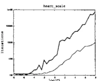
Fig. 1. Number of decomposition iterations for solving SVM with linear (the thick line) and RBF (the thin line) kernel

updated. We will show that the situation is even worse when solv- ing linear SVMs.

It has been demonstrated (e.g. [51) by experiments that if G is large and the Hessian matrix Q is not well-conditioned, decompo- sition methods converge very slowly. For linear SVMs, if n

<<

1, then Q is a low-rank matrix which is not well-conditioned. When C is large, we can see the number of decomposition iterations dra- matically increases. The situation is much worse than that for non- linear SVMs. In Figure 2.1, we demonstrate a simple example by using the problem heart from the statlog database. Each attribute isscaledto [-1, 11. WeuseLlBSVM [ I ] tosolvelinearandnonlin- ear SVMs (RBF kemel, e ~ l ~ z ~ ~ ~ ~ ~ l z ~ ~ * o z ~ with 1 / ( 2 c 2 ) = l / n ) with C = 2-', 2 - 7 . 5 , . . . ,2' and present the number of item- tions. Though two different optimization problems are solved (in particular, their Q.j's are in different ranges), Figure 2. I clearly in- dicates the huge number of iterations for solving the linear SVM. In the following, we give some theoretical explanation about this difficulty.

For problems which are not linearly separable, [7] proved the following result:

Theorem 1 There exists

afifnite

value

c

'

and ( w * ,

b')

such that

( w , b ) = ( w * , b') solves ( I ) afrer C

2

C'. In addition,

xi=,

E.

is a consranr after

C

2

C'.

Therefore, after

C

2 c',

aTQa

= wTw becomes a con- stant. Since $ w T w

+

c

Et=,

<.

= eTa - ~ Q ' Q U , after

c

2

c',

$aTQa

- eTa is a linear decreasing function of C. It has been shown in [ I O ] that, under some conditions, a com- monly used decomposition method is linearly convergent. There- fore, using the zero vector as the initial point, the smaller the opti- mal value is, more decomposition iterations are needed.

Though linear SVM with n

<

1 does not satisfy the assump- tions in [IO], if it is still linearly convergent, when

C

is large,

i a T Q a

- eTa decreases linearly with

C.

This results in the dif- ficulty that the number of decomposition iterations may increase linearly.

Furthermore, [IO, Section 41 explains that the linear conver- gence rate of linear SVMs is relatively smaller than that of non- linear SVMs whose kernel matrices are well-conditioned. This indicates that decomposition methods is inherently not suitable for linear SVM due to its slow convergence.

2.2. Special Implementation for Linear SVMs

Though we have shown a disadvantage of using decomposition methods for linear SVMs, for practical implementations, there are special properties of linear SVMs which can speed up each itera- tion.

Most decomposition implementations maintain the gradient vector of the dual objective function during iterations. It is used for

selecting the working set or checking the stopping condition. We usually calculate the gradient

Qa

- e by the following way: Sup- pose

,'+'

and a* are solutions of two consecutive decomposition iterations, Qa*+'-e = Qa*-e+Q(a'+'

-a*).

Since f r o m a ' to a*+', only q components are changed, Q(a*+' -

a * )

involves with q columns of the matrix Q . Far a non-linear SVM where Q is too large to be stored in the computer memory, the calculation of

lq kemel elements becomes the main computational cost in each decomposition iteration. If each kernel evaluation requires

O ( n )

operations, O(1nq) is the complexity of each iteration.

However, for linear SVM, Q(a"+' - a ' ) = X T ( X ( a " + ' ~

a')),

where

X

= [ylxl,.

. .

,

ylxl] is an n by 1 matrix. Thus, XJa'+l ~ a') involves O(nq) operations and X T ( X ( a * + ' ~

a

)) needs O(1n). Therefore, O(1nq) operations are largely re- duced to

O(1n).

The first decomposition software which imple- ments this for linear SVM is SVM1*gh' [6]. Another implementa- tion is BSVM 151.

However, for SMO [14] implementations where q = 2, the main cost of each iteration is only reduced by half. From this

as-

pect, SMO type implementations are particular not suitable for lin- ear SVM. In other words, using a larger q, the cost on updating the gradient is the same but the number of iterations is smaller. Thus, we should increase q until the cost of solving the sub-problem (usually O ( q 3 ) ) becomes a dominant part.

3. ALPHA SEEDING FOR LINEAR SVM

Results in [7] show the following properties of the dual linear SVM: There is

6'

such that for all

C

2

C', there are optimal so- lutions at the same face. In addition, for all C

>

C', the primal so- lution w is the same. The definition that two points are at the same face is as follows: Let

a'

be a feasible vector of (2) for

C

= C1 and

a'

be a feasible vector of (2) for C = CZ. We say that a' and a2 are on the same face if the following hold: (i)

{i

I

0

<

at

<

C,} =

{Z

1

0

<

a1

<

Cz}; (ii)

{Z

I

at = C,} = {i

1

a1 =

G } ;

and, (iii)

{i

1 ai

= 0) = {z

I

a;

= 0 ) . Therefore, a face means a partition of {l,

. . .

, 1 } to three sets where corresponding components of a are free, upper-bounded, and lower-hounded.

Based on these properties, we conjecture [hat for large C , op- timal solutions are at similar faces. Therefore, if

a'

is an optimal solution at C = Cl, then a'C,/C, can be a very good initial point for solving (2) with C = CZ. This technique, called alpha seed- ing, was originally proposed for SVM model selection [4] where

several (2) with different C have to be solved.

Earlier work which focus

on

nonlinear SVMs mainly use alpha seeding as a heuristic. Now for linear SVMs, a'C2/CI is at the same face as

a'

so most likely it is at a similar face of one optimal solution of

C

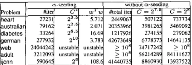
= CZ. This strongly supports its use as the initial solution.

Next, we conduct some comparisons between the proposed and the original implementations. Here, we consider two-class problems only. Some statistics of the data set used are in Table 2.

We train linear SVMs with

C

=

[Z-',

Z - 7 . 5 , .

.

. ,2']. Table I presents the total number of iterations of training 33 linear SVMs using the alpha seeding approach. There are quite a few implemen- tation considerations. Here, the code is modified from LIBSVM; details are in [2]. We then individually solve 33 problems and list the number of iterations (total, C = 2'.5, and C = 2'). For the new approach, we also list lhe approximate C' for which linear SVM with

C

2

C' have the same decision function. In addition, the constant w T w after C

?

C' is also given. For some problems

Table 1. Comparison of iterations (linear kernel); with and without alpha seeding.

Table 2. Comparison of iterations (RBF kernel); with and without alpha seeding.

(e.g. web and adult),

w T w

has not reached a constant until C

is

very large

so

we indicate them as “unstable” in Table I It can be clearly seen that the alpha seeding approach performs

so well to the point that its total number of iterations is much less than solving one single linear SVM with the original decomposi- tion implementation. Therefore, even if we intend to solve one linear SVM with a particular C, using the proposed alpha seeding method starting from a smaller

C

may be more efficient.

Our experimental results indicate that the slow convergence of decomposition methods causes a huge number of iterations for changing some initial zero components to the upper hound

C.

On the other hand, the new approach starts from a small C where an optimal solution can be easily obtained. Then, as the next

C

is only slightly increased, the optimal solution face is not changed much. Hence, using the previous solution multiplied by the increase of C as initial points, the saving on the number of iterations is dramatic. Furthermore, since we have solved linear SVMs with different

C, model selection by cross validation is already done. To be more

precise, we can randomly separate data

to

different folds first. If one fold is singled out as the validation set, we sequentially train the rest and predict the validation set using different

C.

This will he discussed in Section 5 .

To demonstrate that alpha seeding is much more effective for linear than nonlinear SVMs, Table 2 presents the number of iter- ations using the RBF kernel K ( z i , z j ) = e - ~ l z . - z i ~ ~ z / ( z a z ) with 1/20’ = l / n . It can be clearly seen that the saving of iterations by using alpha seeding is marginal. In addition, comparing the “total iter.” columns of both tables, we confirm again the slow convergence for linear SVMs if without alpha seeding.

To further justify the alpha seeding approach for linear SVMs, in [2] we prove the following theorem:

Theorem

2

Assume that any two parallel hyperplanes in the fea- ture space do nor conrain more rhan n

+

1 points of {xr} on them.

We have

1. For any optimal solution of (Z), if has no more than n

+

1 free componenrs.

2. There is C’ such rhar +er C

2

C’, all optimal solutions of

(2)

share at least fhe same 1 - n - 1 upper and lower- bounded a variables.

This result indicates that if n

<<

1,

starting from small C, most components of optimal solutions are at bounds. From any

61

to C,, even if all free components are different, two solutions share at least 1 - 2(n

+

1) bounded variables. If Cz is not far away from C1, it is less likely that an upper (lower) component at

61

becomes a lower (upper) bound at

CZ.

Thus, it is highly possible that the initial solution by alpha seeding has correctly identified at least 1 ~ 2(n

+

1) components of an optimal solution.

Theorem 2 also helps to explain why web is the most difficult problem for results in Table 1. Its large number of attributes might lead to more free variables during iterations or at the final solution. Thus, alpha seeding is less effective.

Another result which supports the use of alpha seeding is the following theorem:

Theorem 3 There are two vecrors A,

B,

and a number C’ such thatfor any C

2

C’,

AC

+

B is an optimal solution of(2). The proof is in [21. This theorem extends the result in 171 which shows only that for any C

>

C‘, there are optimal solutions a which form a linear function of

C on

the interval

[C‘,

c].

Clearly Ai

2

0 so we can consider the following three situations of vectors A and

B:

For the second case, at

2

=

A,Cz

+

E ;

= 0. For the first case, A;C

>>

B;

after

C

is large enough. Thus,

a t 2

= AiCz

+

Btg x A ; C z

+

B;. Using Theorem 2, there are few (< n

+

1) components satisfying the third case. This analysis also shows the effectiveness of using alpha seeding.

1. 0

<

A,

5

1, 2. A; = 0 , B ; = 0,

3.

A; = 0,B;

>

0.

4. COMPARISON WITH OTHER APPROACHES

Table 3. Comparison of approaches for linear SVMs (time in sec- ond; q : size of the working set of decomposition methods.)

It is interesting to compare the proposed approach with other methods. In particular, there are approaches which are mainly suit- able for linear SVMs. In this section, we consider Active SVM (ASVM) [12] and Lagrangian SVM (LSVM) [13].

LIBSVM, the software used in Section 3, implements an SMO- type decomposition method where in each iteration two variables are updated. For problems with more free variables at final so- lutions, many such updates (i.e. iterations) are needed. As now the number of free variables is generally less than n

+

1 and most bounded variables have been identified in the beginning using al- pha seeding, we suspect that a decomposition method with a larger working set can benefit more from the alpha seeding. Thus, here we implement it in another decomposition software BSVM [51 which allows an arbitrary size of the working set.

However, BSVM. ASVM, and LSVM all solve slightly dif- ferent formulations from (1 ). (Due to space limit, we discuss the difference of their implementations in [Z].) Thus, it is very difficult to conduct a fair comparison. Our goal here is only to demonstrate

that decomposition methods, which are originally unsuitable for solving linear SVMs, can be competative with other linear-SVM methods, using the proposed implementation. Table 3 presents a comparison of the four implementations. We use the same bench- mark problems as in Section 3 . The computational experiments were done on a Pentium 111-I000 with 1024MB RAM using the gcc compiler.

For each problem, linear SVMs with C = 2-', 2 r ' . 5 , . . . ,2' are solved. Except the total computational time, we also list the number of iterations of the two decomposition implementations. Clearly for problems with small n, for each C , BSVM takes very few iterations. The computational time is also less than that of LIBSVM. T h i s is consistent with our earlier statement that for linear SVMs, SMO-type decomposition methods arc less favorable than general decomposition methods with larger working sets.

Since alpha seeding is not applied to ASVM and LSVM, we admit that their computational time can be improved. Results here also serves as the first comparison between ASVM and LSVM. Clearly ASVM is faster. Moreover, due to the huge computational time, we set the maximal iterations of

LSVM

to be 1000. For problems adult and web, after C is large, the limit of iterations is reached before stopping conditions are satisfied.

5.

EXPERIMENTS ON MODEL SELECTION If the RBF kernel is used, 17) proposes the following model selec- tion procedure for finding good

C

and U ' :

1. Search far the best C of linear SVMs and call it

6.

2. Fix

C

from step 1 and search for the best (C, U ' ) satisfying

log U' = log

C

~ log

6

using the

RBF

kernel.

That is, we solve a sequence of linear SVMs first and then a se-

quence of nonlinear SVMs with the KBF kernel. The advantage of

this approach over

an

exhaust search of the parameter space

is

that only parameters on two lines are considered. If the original decom- position method is used for both linear and nonlinear SVMs here, due to the huge number of iterations, solving the linear SVMs be- comes the bottleneck. Our goal in this section is to show that using the new approach for linear SVMs, the computational time spent on the linear pan is no longer a problem.

Earlier in [7], due to the difficulty on solving linear SVMs, only small two-class problems are tested. Here we would like to evaluate this approach on large multi-class datasets. We consider four problems: d n a , satimage,

letter,

and shuttle. Details of our settings are in

[21.

We search for

6

by five-@Id cross validation on linear SVMs using uniformly spaced log,

C

value in J-,lO, 101 (with grid space 0.5). Then the search of (log,

C,

log, U ) IS by considering points

in (-2,121 x [-10,4] (with grid space 1) satisfying logu' = log C

-

log

C.

Thus, the number of SVMs solved in two steps may be different.

Table 4 presents experimental results. For each problem, we compare the test accuracy by a complete grid search and the model selection method in [7]. Their performance is very similar. How- ever, the total model selection time of the new method is much shorter. We achieve this because using the alpha seeding, solving one linear SVM is as fast as solving a non-linear one. Otherwise, time for solving linear SVMs is a lot more so the proposed model selection method does not possess any advantage.

Table 4. Comparison of different model selection methods (time in

second; "Linear(#SVMs):" time for linear SVMs and the number of linear SVMs solved.)

6. CONCLUSION

In conclusion, we hope that based on this work, SVM software using decomposition methods can be suitable for all types of prob-

lems, no matter n

<<

1 or n

>>

1.

7. REFERENCES

111 C.-C. Chang and C:J. Lin. LIBSVM: a l i b m n , f o r

support vector machines. 2001. Software available at

http://www.csie.ntu.edu.t~/-~jlin/libsvm.

[21 K:M. Chung, W.-C. Kao. T. Sun, , and C.-I. Lin. Decompasi- tion methods for linear suppon vector machines. Technical repon. Depanment of Computer Science and Information Engineering, Na- tional Taiwan Uniuersity, 2002.

[3] C. Cones and V. Vapnik. Suppon-vector network. Machine Learning.

20273-297. 1995.

[4] D. DeCoste and K. Wagstaff. Alpha seeding for support vector ma- chines. In Proceedings of lnfernalionol Conference on Knowledge

Discovery and Dora Mining (KDD-ZOOO), 2000.

[ 5 ] C.-W. Hsu andC.-J. Lin. A simple decomposition method for support

vector machines. Machine Learning, 46291-314, 2002.

I61 T. Joachims. Making large-scale SVM learning practical. I n

B.

Schhlkopf, C. J. C. Burges, and A. 1. Smola, editors, Advances in Kernel Methods - Suppon Vecror Leorning, Cambridge. MA, 1998. MIT Press.

171 S. S . Keenhi and C . ~ J . Lin. Asymptotic behaviors of

suppon vector machines with Gaussian kernel, 2002.

http://uniw.csie.ntu.edu.tw/-cjlin/papers/limit.ps.gz.

[SI S. S. Keenhi, S . K. Shevade. C. Bhattacharyya, and K. K. K. Murthy.

A fast iterative nearest point algorithm far suppon vector machine classifierdesign. 1EEETrnnsoclionson Neural Nerworks, 13(1):124- 136,2000.

191 Y.-I. Lee and 0. L. Mangararian. RSVM Reduced suppon veclor machines. In Proceedings of the First SIAM lnrernotionul Conference

on Data Mining, 2001

I101 C.-J. Lin. Linear convergence o f a decomposition method far suppon vector machines. Technical report, Depmment of Computer Science, National Taiwan University, Taipei, Taiwan, 2001

[Ill K.-M. Lin and C.-J. Lin. A study on reduced support vector ma-

chines. Technical repon, Department of Computer Science and In-

formation Engineering, National Taiwan University, Taipei, Taiwan, 2002.

1121 0. L. Mangasmian and D. R. Musicant. Active set support vector ma-

chine classification. In Advances in Neural Information Processing

Systems, pages 577-583, 2000.

I131 0. L. Mangararian and D. K. Musicant. Lagrangian suppon vector machines. JournalofMachim Learning Rerearch, 1:161-177,2001.

[I41 J. C. Platl. Fast training of support vector machines using sequential minimal oolimiration. In B. Schiilkoaof. C. J. C. Burma. and A. J.