As an alternative to the application of the standard coherent

Chapter 4

PolSK Modulated Harmonic Mode-Locked Fiber Ring Laser

In this chapter, we purpose to generate the optical pulse train with higher repetition rate than modulation frequency. This paper is organized as following: Section 4-1 introduces the background of the polarization shift keying and experimental motivation. In section 4-2, we explain the physics and principle of the polarization shift keying. In section 4-3 we discuss system description and polarization shift keying present the experimental results. In section 4-4 we give the summary.

4-1 Introduction

As an alternative to the application of the standard coherent

modulation techniques like ASK, FSK, PSK and DPSK to coherent

optical communications, modulation methods exploiting the vector

characteristics of the propagating light radiation have been recently proposed and/or experimentally demonstrated in laboratory [42-45].

They use the state of polarization (SOP) of a fully polarized lightwave as

the information-bearing parameter, exploiting the two orthogonal

channels available in free space as well as in a single-mode fiber

propagation. In free space, two orthogonal input signals maintain their

state of polarization while propagating. In the case of single-mode fibers

fed by a monochromatic light source, orthogonal SOP pairs at the input

lead to orthogonal output SOP pairs, although the input state of

polarization is not maintained in general. Moreover, careful

measurements reported in [46-47], and [48] have shown that

depolarization phenomena or polarization dependent losses are of little

importance even after relatively long fiber spans. These properties are

crucial to digital modulation based on SOP, called Polarization Shift

Keying (POLSK). Demodulation and detection is accomplished through

the analysis of the SOP. A SOP is fully described by the knowledge of the

Stokes parameters. People Stokes receiver as a coherent heterodyne

receiver extracting the Stokes parameters from the IF signals. All

proposed POLSK systems make use of a binary modulation scheme

(2-POLSK), i.e., information is sent by switching the polarization of the transmitted lightwave between two linear orthogonal SOP’s. In the three-dimensional space defined by the Stokes parameters two orthogonal.

Thus, detection of binary modulation schemes is simply accomplished by

looking at the sign of the scalar product of the received SOP vector in the

Stokes space with a reference vector representing one of the received

SOP’s in the absence of noise. This reference vector depends on the fiber

induced changes on the transmitted SOP’s and for this reason all 2-PolSK

systems must somehow keep track of it. While the system outsketched in

[49] exploits the S

path. A complete Stokes receiver is used by the

system proposed in [50]. A fourth interesting scheme

(JMPSK) has been

presented in [51], which uses a rather different signal processing. All

these schemes can he viewed as POLSK systems. The above-mentioned

reference recovery is accomplished electro-optically. This implies that

they can make use of only part of the Stokes receiver because it is

supposed that active electro-optic controls force the received SOP’s to

align with a specific axis of the receiver Stokes space reference. The third

and fourth systems, which will be shown to be equivalent, perform an

electronic reference recovery by means of long-term averages over the

received signals.

All the known results place PolSK modulation, in terms of required power, between ASK and DPSK, with a theoretical degradation of 3 dB with respect to DPSK in the absence of laser phase noise.

As to the effect of the laser phase noise, a general analytical treatment in coherent optical heterodyne receivers is not available. However, numerical analyses and experimental results have proved the considerable insensitivity to phase noise of receivers based on non-linear memoryless processing of the signal. That the IF filter bandwidth is large enough to avoid phase-to-amplitude noise conversion [52-54]. PolSK schemes can be thought of belonging to this class of systems, also called PNCHR (phase-noise-canceling heterodyne receivers) [55].

4-2 Theory of PolSK

The state of polarization (SOP) of a fully polarized light- wave can be described through the Stokes parameters. Given a reference plane , normal to the propagation axis of an electromagnetic field, the expression of which is [56]

y x ˆˆ,

zˆ

)) (

)

(

x x

e

t a

E =

)) (

)

(

y y

e

t a

E =

y E x E

E ˆ =

ˆ +

ˆ (4-1)

The Stokes parameters can be calculated as follows[57]:

2 2

1

a

a

S = −

) cos(

2

2 a

a

δ

S =

) sin(

3

2 a

a

δ

S = (4-2)

with

y

x

φ

φ

δ = − (4-3)

In (4-2) we have omitted the dependence on time of the parameters for notational simplicity. This will be used throughout the paper in all unambiguous cases.

In classical optics an average is generally taken of the quantities appearing in the right hand side of (4-2). For our use we assume (4-2) to define “instantaneous” values for these parameters. A fourth parameter[58]

(4-4)

2 2 2

0

a

a

S = +

represents the total electromagnetic power density traveling in the zˆ

direction. The following also shown as:

(4-5) The S

2 3 2 2 2 1 2

0 S S S

S

= + +

i

can be represented in a three-dimensional space with unit vectors . We will call this space “Stokes space.” For waves having the same power density, lies on a sphere of radius , called

“Poincare sphere”. A fundamental feature of this representation is that SOP’s orthogonal according to the hermitian scalar product[59]:

3 2 1, ˆ , ˆ

ˆ S S

S

Sˆ S₀

) ( )

)

ˆ ( ˆ ˆ

ˆ ′ ⋅ E ′′ = v ′ ⋅ v ′′ a ′ a ′′ e

e

E (4-6)

map onto points which are antipodal on the Poincare sphere. Moreover all linear polarizations lie on the (S

. S

) plane, while the points

represent the two possible circular SOP’s. The other points represent elliptic SOP’s.

We will prove in the following that the performance of every receiver operating on the Stokes parameters obtained from a received signal perturbed by additive white Gaussian noise (AWGN) are invariant with respect to the choice of the reference system in the receiver, or, equivalently, with respect to the modifications induced by the fiber onto the SOP.

3 0

ˆs

± S

3 2 1

, ˆ , ˆ

ˆ S S

S

We assume that the power of the local oscillator is equally split between the and channels. Shot noise processes appearing on the and

. IF channels after photodetection can be written as [60]:

x

x

y

) sin(

)

cos( w t x w t

x

x =

−

) sin(

)

cos( w t y w t y

y =

−

(4-7)

where are independent white Gaussian random processes with power spectral density N

s c s

c

y

x

,

0. In optical systems, the received field is

generally affected by phase noise, and so is the local oscillator. Up to now, a general analytical treatment of phase noise in receivers that use band - pass filtering and then non-linear processing of the signal, as in Stokes receiver branches, is not available. However, in such receivers, under reasonable hypotheses, phase noise can be considered to be suppressed to a great extent. These hypotheses are:

(a) ideal square-law elements, or multipliers;

(b) IF filter bandwidth “large enough” with respect to the IF beat linewidth to avoid phase noise to amplitude noise conversion.

The “large enough” criterion means that in general it is necessary to allow

for a wider IF bandwidth than the one that would be chosen on the basis

of the information signal spectrum only. However, wider IF filter bandwidths mean larger noise power, thus a certain penalty has to be expected. It can be significantly reduced by the use of a filter. Under (a) and (b), phase noise cancels Out within the nonlinear elements, where only products of synchronous signal components are performed. In the following treatment we will assume that (a) and (b) hold. However, even under this assumption, in the mathematical expressions of the baseband signals of a generic receiver employing square-law devices or multipliers, phase-noise does not cancel in signal-times-noise terms. This leads to rather involved formulas, although, once the statistical properties of these terms are analyzed, it turns out that they are not altered by the presence of phase noise factors. To get rid of these complex noise expression, and to prove that under a) and b), phase noise no longer affects these systems, we first get back to the original shot noise processes (3-7). We state that expressing shot noise through

(4-8) (where

t t jw

t j w

e x e

x ˆ ′

= ˆ

)

n(t

φ

represents the phase noise, a random process independent of ), the process . has identical statistical characteristics as . The

xˆ x′ ˆ xˆ

same holds for

ˆ . To prove this, we express x

′, x

′ as a function of . We get [61]

s

c

x

x ,

⎥ ⎦

⎢ ⎤

⎣

= ⎡

⎥ ⎦

⎢ ⎤

⎣

⎡

′

′

s c s

c

x U x x

x (4-9)

where U is

⎢⎣

⎡ t t

n n

φ φ cos

sin _⎥

(4-10)

⎦

⎤

− t

t

n n

φ φ sin cos

a real unitary stochastic matrix. Now, we resort to the following theorems, whose proof is reported.

Theorem 1: given two independent real zero-mean stationary random processes, jointly Gaussian and identically distributed, say a and b, and the transformation:

(4-11) where U is a real unitary matrix, the processes a’ and b’ are still independent zero-mean Gaussian random processes with the same distributions as a and b.

Theorem 2: assuming all the hypothesis of (T1), except for U that is now a stochastic unitary matrix, in the sense that its coefficients are stationary random process independent of a, b,. such that

⎥⎦

⎢ ⎤

⎣

= ⎡

⎥⎦

⎢ ⎤

⎣

⎡

′

′

b U a b a

1 ) ( )

( =

+ t U t

U

(4-12)

(T1) still holds if and only if a, b are white random processes. It is straightforward to verify that (Tl) and (T2) prove (4-8).

Once this equivalent representation has been adopted, phase noise factors cancel out of noise-times-signal terms in much the same way as they cancel out of signal-times-signal terms. Hence, under (a) and (b) the systems has a complete immunity with respect to phase noise, and this tolerance is mirrored in baseband formulas where all phase noise related terms disappear.

Let us now assume that the incoming field polarization is linear and aligned with one of the analysis axis, say , of the Stokes receiver.

Baseband expressions of the Stokes parameters are in this case:

xˆ

2 2 2

2 2

1

A 2 Ax

x

x

y

y

S = + + + − −

c s

s c

c

y x y Ay

x

S

= 2 ( + ) + 2

c s

c c

s

y x y Ay

x

S

= 2 ( + ) + 2 (4-13)

This assumption implies that the signal, intended as a term where noise

factors are absent (i.e.,

only. The set (4-13) is a very neat and readable form of the output of the Stokes receiver. When the signal SOP, however, instead of being linear and aligned with , is of a general form, this simple form becomes more complicated and results in expressions where all the S

xˆ

i

’s display both noise and signal terms. Nevertheless, we will show that the analysis of noise statistics and, as a consequence, of PolSK systems performance can be carried out on just the simple (4-13) form, without any loss of generality.

To prove this we first introduce the Cayley-Klein [62] representation of a rotation of the reference system in a three dimensional space:

⎢⎣

⎡

= +

3 2 1

jS S

P S

(4-14)

(4-15)

⎥⎦

⎤

−

− 1

3 2

S jS S

⎢⎣

⎡ + ′

′

= ′

′

3 2 1

S j S

P S ⎥= ⁺

⎦

⎤

− ′

− ′

′ QPQ

S S j S

1 3 2

where P is the matrix representation of a point of coordinates (S

. S

. S

) with respect to the reference set . , and Q is a rotation matrix such that P’ is the matrix representation of P according to a new reference set . For a theoretical treatment of this formalism.

3 2

1

, ˆ , ˆ

ˆ S S

S

3 2

1

, ˆ , ˆ

ˆ S S

S ′ ′ ′

In this context we need only to know that Q is capable of performing all possible rotations of the reference axes, and that it is a unitary matrix with the additional constraint of a unit determinant.

A way to represent a generic transformation of the SOP of a fully polarized lighwave, which preserves the degree of polarization, is the following. Given E r

E′ r

, the

electromagnetic field vectors before and after the transformation, and given their decomposition:

)) ( ( ₀

)

(

x x

e

t a

E =

E

′ = a

′ ( t ) e

)) ( ( ₀

)

(

y y

e

t a

E =

E ′

= a ′

( t ) e

(4-16)

where X,Y and X, Y are transverse reference axis sets(i.e., normal to the direction of propagation), we have

⎥ ⎦

⎢ ⎤

⎣

= ⎡

⎥ ⎦

⎢ ⎤

⎣

⎡

′

′

y x y

x

E Q E E

E

(4-17)

where Q is a complex matrix with unit determinant called Jones matrix. A

subset of Jones matrices, called the set of matrices of birefringence or

optical activity, not only preserves the degree of polarization, but also has

the additional feature of preserving orthogonality (according to the

Hermitian scalar product) between two fields which are orthogonal before the transfomation. Matrices of this kind are complex unitary matrices with unit determinant. Throughout this paper, when talking of Jones matrices, we strictly refer to this latter subset.

Calling S r

the SOP vector of the E r

field and S′ r

the SOP vector of the E′ r

field, with S r

and S′ r

expressed according to Stokes references consistent with the x r , y r _and, x r , ′ r y ′ geometrical reference axes, we associate to S r

and S′ r

their matrix representation P

P′

respectively, according to (4-14).

The proof of this result, in the framework and with the notations of this paper, is given in Appendix A. In a more general and abstract. To implies that a generic SOP transformation which preserves the degree of polarization is equivalent to a rotation of the reference axes in the Stokes space. If this rotation is expressed through the Cayley-Klein formalism, the corresponding rotation matrix Q coincides with the Jones matrix.

Let us now get back to the original problem of the generality of the (4-13)

form. We assume that x r , ′ r y ′ coincide with the analysis axes of a

Stokes receiver. Consequently, the IF-stage signal vector in the Stokes

receiver is, according to the notation (4-2) and dropping a constant factor:

⎥ ⎦

⎢ ⎤

⎣

= ⎡

⎥ ⎦

⎢ ⎤

⎣

⎡

′ + ′

⎥ ⎦

⎢ ⎤

⎣

⎡

ch ch y

x

y x E

E y

x

(4-18)

where are the analytic signal representation of the noise processes and are the noisy signals on the IF-branches of the Stokes receiver.

Now, we assume that: (a) the fiber does not affect the degree of polarization of the field;(b) the fiber does not induce loss of orthogonality between two orthogonal (according to the Hermitian scalar product) input fields. Assumptions (a) and (b) stem from the results of experimental and theoretical works, such as [63], which have demonstrated that depolarization effects or polarization- dependent losses are to a great extent negligible in optical fibers. Under the above-mentioned hypotheses, it is always possible to write (3-18) as follows:

y x r , ′ r ′

ch ch y x ,

(4-19)

⎥ ⎦

⎢ ⎤

⎣

= ⎡

⎥ ⎦

⎢ ⎤

⎣ + ⎡ ′′

⎥ ⎦

⎢ ⎤

⎣

⎡

ch ch

y x Q E

y x

0

where Q is a Jones birefringence matrix that changes the field SOP in such a way to transform a field linearly polarized along .x in the arbitrary reference x r , ′′ r y ′′ into the received field

r

′

r ′

,

From (4-19) we can write:

⎜⎜

⎝

⎛ ⎥

⎦

⎢ ⎤

⎣

= ⎡

⎟⎟⎠

⎥⎞

⎦

⎢ ⎤

⎣ +⎡ ′′

⎥⎦

⎢ ⎤

⎣

⎡

′′

′′

ch ch

y E x

y Q x

0

(4-20)

with:

(4-21)

⎥ ⎦

⎢ ⎤

⎣

= ⎡

⎥ ⎦

⎢ ⎤

⎣

⎡

′′

′′

x ₁

4-2-1 Performance of PolSK Modulation Schemes

Let us now compute the performance starting from the expression (4-13) of the Stokes parameters. We will try first to characterize the received noisy vector

with respect to the unnoisy one

SrI

. In practice, we are substituting in finding the conditional of the receiver output given the ideal unnoisy one

)

\

\S ( N I

S S S

f

I N

r

r r

r

(4-25)

To do this, we shall take the unnoisy signal unit vector, which according to (4-13) is

, as the polar axis of a polar reference with

respect to which

will have components:

) , , (

θ α

r

≡

The angle θ can be expressed as follows

⎟⎟

⎟

⎠

⎞

⎜⎜

⎜

⎝

⎛ ⋅

=

I N

I N

S S

S S r r r r cos

θ (4-26)

Calling

the projection of

over the plane orthogonal to , and chosen a unit vector over this plane

SrI

Srα

we have:

⎟⎟

⎟

⎠

⎞

⎜⎜

⎜

⎝

⎛ ⋅

=

⊥

− N

I N

S S S

r

r r cos

α (4-27)

We will assume

α =

in the reference used in (4-13). Our aim is to fully describe the statistical properties of the random variables

α θ

ρ , , .The distribution of p is a noncentral chi-square with four degrees of freedom and noncentrality parameter A

[64]is

) (

) 2 (

) 1

(

2

σ

σ

y A I A e

y y f

y A p

− +

= (y>0) (4-28)

And the cdf

) (

1 )

( ₂

σ σ

A y Q y

F_p = − ⋅

(4-29)

Where Q

is a generalized Marcum function, of index 2. The angle α is

uniformly distributed over the interval [0,2 π ]. To prove this result we

first define

s c

x b

x A a

= +

=

s c

y d

y c

=

=

(4-30)

Substituting a,b,c,d in

of (3-13) we get

) (

2 3

) (

2 2

ad bc S

bd ac S

−

=

+

=

(4-31)

Theorem 4 (T4): given four real independent Gaussian random processes a,b,c,d, with equal variance and of which as least c,d are zero-mean, a vector in a bi-dimensional space with components

σ

) ,

(

+

−

(4-32)

Forms an angle with respect to a fixed reference axis on its plane which is uniformly distributed over the interval [0,2 π ]. Alternatively, this statmednt can be also formulated substituting a,b to c,d in the sentence.

We know that

⊥ =

. Applying (T4) to

the above-stated result for α is proved. Calculations concerning θ are much more involved.

Through the steps described in detail in Appendix B it’s pdf turns out to be

)]

cos 1 4 ( 1 2 [

) sin

(

2

2 (1 cos ) 2

4

θ

σ

θ θ

θ

=

+ A +

e f

A

θ ∈ [ 0 , π ] (4-33)

Integrating (4-33) we find the even simpler of θ

) cos 1 2 (

1 1 ) (

) cos 1 ( 2 4

2

θ θ

θ

θ

= −

+

− A −

e

F

θ ∈ [ 0 , π ] (4-34)

Finally, we state the following result. The angle α is statistically independent of both θ and

. To show this, we resort to the auxiliary vector representation

2 1

1

a v b v

v r = r + r (4-35)

with a, b random Gaussian processes. The angle α

formed by v r

_with respect to a reference vector, say v r

, and the magnitude are statistically independent random variables.Therefore, since θ depends only on p quantities, which in turn are independent of α

and α

, we conclude that θ is independent of α. For the same reason α is independent of

) ( ρ

ρ

ρ = +

signal-to-noise ratio approaches zero (A→0). Moreover, in that case it can be shown through direct computation of the characteristic function that the pdf of the single Stokes parameter Si is a Laplace one, with parameter

2 2

1 σ

. The statistical characterization of p θ, and α obtained in this

section makes it possible to study the performance of n-POLSK and

d-DPOLSK systems. In the following sections we will exploit these results to derive the error probability for some specific system configurations.

4-2-1 Principles of operation optical

Our electro-optic polarization modulator uses a single waveguide mode converter to switch light between polarization states that lie on the great circle of the Poincaré sphere that contains the horizontal linear polarization state (the H state), the vertical linear polarization state (the V state), and the two poles (the right-handed and the left-handed circular polarization states, the R and L states, respectively), the HRVL circle.

This single waveguide mode converter is a “two-moded” AlGaAs/GaAs waveguide fabricated bricated in (100) GaAs and running in a < 011

> direction. The waveguide is two-moded in that it supports two

orthogonal eigen-modes. Light is launched into one facet of the

waveguide in either the H state, corresponding to the fundamental

TE-like mode, or the V state, corresponding to the fundamental TM-like

mode. This launched, linearly polarized, light is resolved into two

components each of which corresponds to one of the eigen-modes of the

waveguide. By design, these two eigen-modes are linearly polarized at 45

to the horizontal and the vertical directions and correspond to the D and D’. Essentially our polarization modulator is as a TE change TM mode converter followed by a “static” polarization controller. The TE,TM mode converter operates in the following manner. A cross section of the AlGaAs/GaAs waveguide together with the crystal orientation. Application of an electric field in a < 0 1 1 > direction induces changes in the optical indicatrix along the e < 2 1 1 > and < 2 1 1

> directions via the electro-optic effect. These changes are equal but opposite. If, say, light in the H state, the TE-like mode polarized parallel the [0 1 1] direction, is launched into the waveguide it will resolve itself into the D and D’ states, the hybrid eigen-modes polarized in the [2 1 1]

and the [2 1 1] directions. Since in our modulator the differential modal

loss of the hybrid eigen-modes is low, the polarization state at the output

will move along the great circle passing through the poles as the applied

electric field changes. In the conversion from TE to TM, or visa versa, the

polarization state moves along the great circle of the Poincaré sphere that

connects the two points, H and V, on the equator of the sphere through

one of the poles, depending on the direction of the applied field. Using

the polarization modulator, ultrahigh-speed modulation between any two states on the Poincaré sphere can be achieved.

4-2-2 Principles of operation electrical

In order to achieve ultrahigh-speed operation the velocity of the modulating electrical signal must be matched to that of the optical signal and the resistive losses must be kept to a minimum. The velocity of the modulating electrical signal is matched to that of the optical signal by loading the transmission line with fins and pads see[ref 5-6] . The fins and pads add capacitance to the line, without creating a significant change in the inductance, which results in a lower phase velocity or higher microwave index. The microwave index is tailored to be the same as the group index of the optical waveguide at the upper 3 dB point of the modulator.

4-3 PolSK of Harmonic Mode-Locked Fiber Ring Laser Experiment

In harmonic mode-locked fiber lasers, the optical modulator is the

determining component for locking the harmonics of the resonant spectrum into a particular longitudinal mode. For this reason, it is very important to characterize the optical modulator. With detuning the modulation frequency and polarization state, we can get the optical pulse train with repetition rate up to 20 GHz, which is eight times of modulation frequency 2.6 GHz. We proposed to solve the problem by using nonlinear modulation of modulator without adding any other components.

4-3-1 Experimental Setup

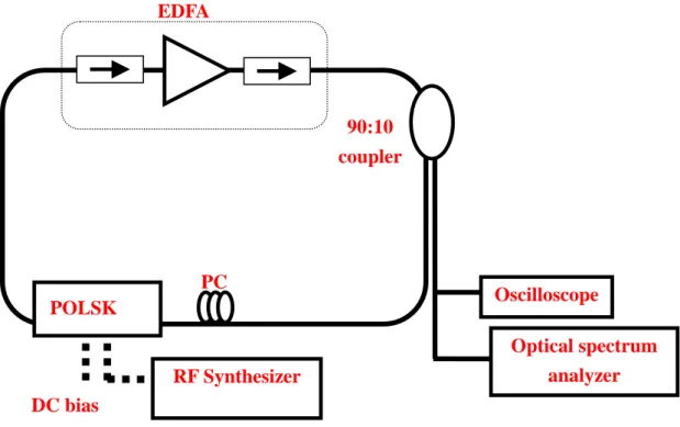
The configuration of the laser is shown schematically in Fig. 4-1. The

cavity length is 21.83 m. The gain media of the ring laser cavity is

provided by an erbium-doped fiber amplifier (Holland Electronic Corp

mount, model NE6000). The output power of the EDFA is 25dBm. There

are two isolators incorporated in the erbium-doped fiber amplifier to

ensure the unidirectional operation of the ring laser. In this structure we

also use 40 GHz polarization shift keying(Versawave-a division of JGKB

Photonics), and then driven by superimposing a sinusoidal signal with

amplitude level of 17 dBm derived from a 2.69 GHz synthesizer (Leader,

modal no. 3221). The laser could be forced to operate stably at harmonic

frequencies of the cavity fundamental mode by detuning the modulation frequency. Because of the somewhat polarization dependent of the modulator, a polarization controller is placed before the modulator to adjust the polarization state of the light for improving the modulation efficiency. The Power is coupled out of the cavity with a 90:10 fiber coupler, where 90﹪of the total power is used as feedback to the cavity, and 10﹪is extracted out from the cavity to measurent. The output spectral and temporal characteristics are measured with an optical spectrum analyzer (Anritsu, modal no. MS9710C) with 0.05 nm resolution, a high speed digital sampling oscilloscope (Agilent, 86100A).

When the polarization controller is correctly adjusted, then various orders of rational harmonic mode-locking can be obtained by only detuning the modulation frequency.

4-4 Experimental Result

In this section, we use the fiber ring to get pulse output and analyze the

result of detuning the modulation frequency. We have tried to adjust the

modulation frequency to measurement the change of pulse train. When

we change modulation frequency from RF generator to observe RMS

jitter and repetition rate. To obtain higher repetition rate, the harmonic mode-locking technique should be used. The phenomenon of pulse train is observed when the modulation frequency is changed.

4-4-1 5 GHz Pulse Train Generation

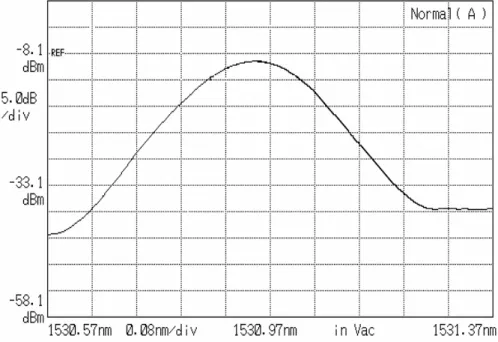
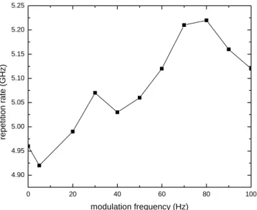
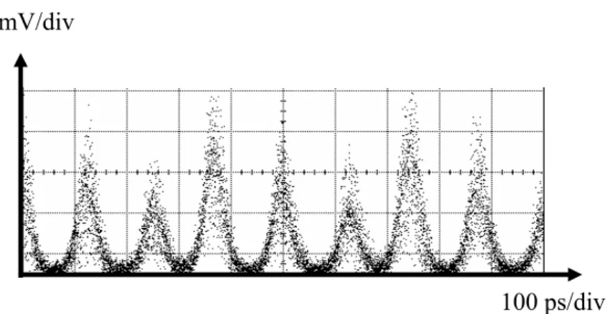
Fig. 4-3 shows the output pulse train of the rational harmonic mode-locked laser when the modulation frequency is set to 2.62334676 GHz. The pulse period is 200 ps which correspond to a repetition rate of 5 GHz and use optical spectrum amplifier to get wavelength as shown as in Fig. 4-4 We also measure the repetition rate in Fig. 4-5 and RMS jitter in Fig. 4-6 by changing modulation frequency. We observe the RMS jitter to find the maximum value of 23.71 ps and minimum value of 23.16 ps.

We alsi observe the rise time Fig. 4-7 to find the maximum value of 14.56 ps and minimum value of 14.18 ps.

4-4-2 7.5 GHz Pulse Train Generation

Fig. 4-8 shows the output pulse train of the rational harmonic

mode-locked laser when the modulation frequency is set to 2.6622143

GHz. The pulse period is 133 ps which correspond to a repetition rate of

7.5 GHz and use optical spectrum amplifier to get wavelength as show as in Fig. 4-9. We also measure the repetition rate in Fig. 4-10 and RMS jitter in Fig. 4-11 by changing modulation frequency. We observe the RMS jitter to find the maximum value of 22.73 ps and minimum value of 18.21ps. We also observe the rise time Fig. 4-12 to find the maximum value of 13.76 ps and minimum value of 12.17 ps.

4-4-3 10GHz Pulse Train Generation

Fig. 4-13 shows the output pulse train of the rational harmonic mode-locked laser when the modulation frequency is set to 2.6423582 GHz. The pulse period is 100 ps which correspond to a repetition rate of 10 GHz and use optical spectrum amplifier to get wavelength in Fig.

4-14 . We also measure the repetition rate in Fig. 4-15 and RMS jitter in Fig. 4-16 by changing modulation frequency. We observe the RMS jitter to find the maximum value of 17.67 ps and minimum value of 16.82 ps.

We also observe the rise time Fig. 4-17 to find the maximum value of 11.81 ps and minimum value of 11.08 ps.

4-4-3 20GHz Pulse Train Generation

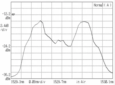
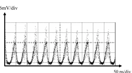
Fig. 4-18 shows the output pulse train of the rational harmonic

mode-locked laser when the modulation frequency is set to 2.65734218 GHz. The pulse period is 50 ps which correspond to a repetition rate of 15 GHz and use optical spectrum amplifier to get wavelength in Fig.

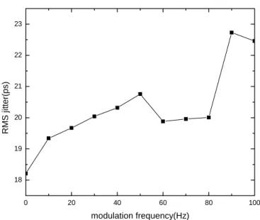
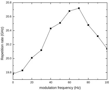
4-19 . We also measure the repetition rate in Fig. 4-20 and RMS jitter in Fig. 4-21 by changing modulation frequency. We observe the RMS jitter to find the maximum value of 14.68 ps and minimum value of 13.81 ps.

We also observe the rise time Fig. 4-22 to find the maximum value of 10.81 ps and minimum value of 9.82 ps.

4-5 Summary

In this chapter, we have demonstrated a new structure of using

amplitude modulated fiber ring laser. We have trigger the mode locked

laser of repetition rate of 5Gb/s, 7.5Gb/s,10Gb/s, 20Gb/s with modulation

frequency of 2.62334676 GHz, 2.66331431 GHz, 2.6423582 GHz,

2.65734218 GHz. In above experiment, we have known repetition

rate ,RMS jitter and rise time changing with modulation.

POLSK

DC bias

RF Synthesizer PC

90:10 coupler

Oscilloscope

Optical spectrum analyzer EDFA

Fig. 4-1 The structure of a phase-modulated

Fig. 4-2 The structure of signal in polarmeter

100 ps/div 6mV/div

Fig. 4-3 The 5 GHz of Polsk mode lock with modulation frequency of 2.62334 GHz

Fig. 4-4 The 5GHz lasing spectrum with modulation frequency of 2.62334 GHz

0 20 40 60 80 100 4.90

4.95 5.00 5.05 5.10 5.15 5.20 5.25

repetition rate (GHz)

modulation frequency (Hz)

Fig. 4-5 Change of repetition rate by detuning modulation frequency

0 20 40 60 80 100

23.1 23.2 23.3 23.4 23.5 23.6 23.7 23.8

RMS jitter (ps)

modulation frequency (Hz)

Fig. 4-6 Variation of RMS jitter by detuning modulation frequency

0 20 40 60 80 100 14.15

14.20 14.25 14.30 14.35 14.40 14.45 14.50 14.55 14.60

Rise time (ps)

modulation freuency (Hz)

Fig. 4-7 Variation of rise time by detuning modulation frequency

6mV/div

100 ps/div

Fig. 4-8 The 7.5 GHz of Polsk mode lock with modulation frequency of 2.66221 GHz

Fig. 4-9 The 7.5 GHz lasing spectrum with modulation frequency of 2.66221 GHz

0 20 40 60 80 100

7.0 7.2 7.4 7.6 7.8 8.0 8.2

repetition rate(GHz)

modulation frequency(Hz)

Fig. 4-10 Change of repetition rate by detuning modulation frequency

0 20 40 60 80 100 18

19 20 21 22 23

RMS jitter(ps)

modulation frequency(Hz)

0 20 40 60 80 100

12.0 12.2 12.4 12.6 12.8 13.0 13.2 13.4 13.6 13.8

rise time (ps)

modulation frequency(Hz)

Fig. 4-11 Variation of RMS jitter by detuning modulation frequency

Fig. 4-12 Variation of rise time by detuning modulation frequency

100 ps/div 6mV/div

Fig. 4-13 The 10 GHz of Polsk mode lock with modulation frequency of 2.64235 GHz

Fig. 4-14 The 10GHz lasing spectrum with modulation frequency of 2.64235 GHz

0 20 40 60 80 100 10.0

10.1 10.2 10.3 10.4 10.5 10.6

Repetition rate (GHz)

modulation frequency (Hz)

Fig. 4-15 Change of repetition rate by detuning modulation frequency

0 20 40 60 80 100

16.8 17.0 17.2 17.4 17.6 17.8

RMS jitter (ps)

modulation frequency (Hz)

Fig. 4-16 Variation of RMS jitter by detuning modulation frequency

0 20 40 60 80 100 11.0

11.1 11.2 11.3 11.4 11.5 11.6 11.7 11.8 11.9

Rise time (ps)

modulation frequency (Hz)

Fig. 4-17 Variation of rise time by detuning modulation frequency

50 ps/div 6mV/div

Fig. 4-18 The 20 GHz of Polsk mode lock with modulation frequency of 2.65734 GHz

0 20 40 60 80 100 19.8

20.0 20.2 20.4 20.6 20.8

Repetition rate (GHz)

modulation frequency (Hz)

Fig. 4-20 Change of repetition rate by detuning modulation frequency

Fig. 4-19 The 20 GHz lasing spectrum with modulation frequency of 2.65734 GHz

0 20 40 60 80 100 13.8

14.0 14.2 14.4 14.6 14.8

RMS jitter (ps)

modulation frequency (Hz)

Fig. 4-21 Variation of RMS jitter by detuning modulation frequency

0 20 40 60 80 100

9.8 10.0 10.2 10.4 10.6 10.8

Rise time (ps)

modulation frequency (Hz)

Fig. 4-22 Variation of rise time by detuning modulation frequency