佇列閾值及寇斯多相統計模型探討與大腸直腸癌早期發現和住院之相關時間分布

(1)

國立臺灣大學公共衛生學院流行病學與預防醫學研究所碩士論文

Graduate Institute of Epidemiology and Preventive Medicine College of Public Health

National Taiwan University Master Thesis

佇列閾值及寇斯多相統計模型探討與大腸直腸癌早期發現和住院之相關時間分布

Queue, Hurdle, and Coxian Phase-type Model for Time Distributions Related to Early Detection and Hospitalization of Colorectal Cancer

任小萱

Grace Hsiao-Hsuan Jen 指導教授：陳秀熙博士

Advisor：Tony Hsiu-Hsi Chen, Ph.D.

中華民國 104 年 5 月

May, 2015

(2)

i

誌謝

在研究所以前，我並未接觸過公共衛生及流行病學領域，很感謝流預所的老師們讓我有機會進入生物統計組來學習這方面的知識。在研究所學習的這兩年，

在老師們細心且專業地指導下，讓我慢慢奠定生物統計的基礎以及培養研究的樂趣，此外我也漸漸體會到公共衛生對於國家社會的重要性，讓我覺得踏上這條路非常的值得。

在這兩年，非常感謝我的指導教授－陳秀熙老師，在老師身上總是可以學到很多，不管是專業上的知識或是生活上的經驗，老師都會毫無保留的與我們分享，

讓我在這兩年過得非常充實、受益良多。這篇論文的完成，最感謝的就是陳老師，

在論文研究及寫作的路上，老師寶貴的指導和建議，幫助我培養自己的思考能力，

能與老師一起做研究是一件非常幸福的事。此外還要感謝嚴明芳老師、陳立昇老師、范靜媛老師以及邱月暇老師，老師們總是在我遇到困難時，給予及時的幫助；

感謝邱瀚模醫師及李宜家醫師讓我從臨床的觀點學習到許多醫學上的知識；感謝我的口試委員張淑惠教授、林明薇教授以及丘政民教授給予我論文寶貴的意見。

在兩年的研究生活，特別感謝研究團隊的許辰陽博士、莊書琳博士、曹慧嫺博士以及蘇秋文學姐，教導我程式技術及學術知識；謝謝思敏幫了我許多忙，我們一起奮鬥、一起努力，有妳在就不孤單；謝謝芸婕總是給我力量，彼此打氣，

有妳的陪伴生活充滿趣味；謝謝琮閔雖然我們都很忙碌，但還是可以互相分享生活點滴；謝謝同學和朋友們，偶爾一起放鬆心情，開心大笑後再繼續往前進。

最後，感謝我的爸媽及家人給予我的支持及鼓勵，提供我最好的環境來學習，

聽我分享生活點滴並回饋給我寶貴的生活經驗，使我越來越強壯，有你們無私的奉獻與愛才有現在的我，我愛你們！

任小萱謹誌于臺灣大學流行病學與預防醫學研究所中華民國 104 年 7 月

(3)

ii

中文摘要

背景

台灣大腸直腸癌的發生率逐年增加，對於大腸直腸癌的早期發現可以先透過糞便潛血檢查再進一步地接受大腸鏡來進行確診，在確診為大腸直腸癌病人後，

後續的住院治療這些都是不容忽視的問題。然而為了考慮民眾的篩檢到達率、未接受大腸鏡確診者的特性、等待接受大腸鏡確診的時間以及大腸直腸癌病人接受後續住院治療的住院天數，傳統的佇列模型是無法實行的。

研究目的

本論文的研究目的是將佇列過程、閾值模型以及寇斯多相模型整合為一個統計方法，並將此方法應用在分析台灣全國大腸直腸癌篩檢之陽性個案所需進行大腸鏡確診的等待時間以及大腸直腸癌病人的住院天數。

研究方法

閾值模型由邏輯斯迴歸以及截尾卜瓦松迴歸模型所組成，邏輯斯迴歸用來研究未接受大腸鏡確診者的特性，截尾卜瓦松模型則用來分析等待接受大腸鏡確診的時間分布。而寇斯多相模型可以探討等待時間的最佳隱藏階段，處理接受轉介民眾之間的異質性。為了可以更進一步地考慮民眾的篩檢到達率，我們結合了卜瓦松過程、閾值模型以及寇斯多相模型進而發展出一個佇列閾值寇斯多相模型。

在住院治療方面，我們利用寇斯多相模型對 178 位大腸直腸癌病人的住院天數進行分析，探討其最佳的隱藏階段個數。

結果

第一部份：在篩檢前期（2004-2009 年），閾值模型的結果顯示女性、年齡較高者、

居住在東部、離島或非都會區民眾、在醫院進行篩檢的民眾或是盛行篩檢個案（首

(4)

iii

次參與篩檢）有較高的機率不接受後續轉介，而居住在中部或大都會地區、在衛生所或健康服務中心接受篩檢的民眾或是非首篩個案其所需等待接受大腸鏡確診的時間較短。

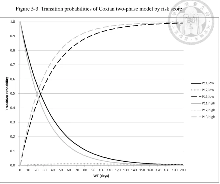
第二部份：在佇列閾值二階段寇斯多相階段模型中，等待大腸鏡確診的時間可被分類為等待時間較短階段以及等待時間較長階段，其結果顯示民眾的篩檢到達率每人天為 0.00021，不接受後續確診的機率為 0.26，一年大約有 15% 的民眾對於後續大腸鏡的確診會猶豫不決而陷入等待時間較長的階段。在等待時間較短階段的平均等待時間為 32 天而在等待時間較長階段的平均等待時間為 169 天。當我們將危險分數考慮到模型中進行分析時，佇列閾值二階段寇斯多相階段模型顯示低分群在等待時間較短階段的平均等待時間為 36 天而高分群為 30 天，在等待時間較長階段，兩群的平均等待時間皆為 167 天。

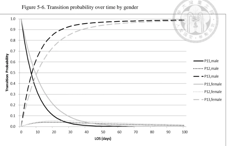
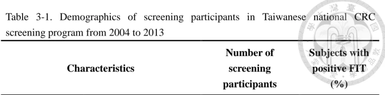
第三部份：在住院治療方面，我們利用三階段寇斯多相模型對 178 位大腸直腸癌病人的住院天數進行分析，住院天數可被分為短期停留階段、中期停留階段及長期停留階段。在短期停留階段中，平均住院天數為 10 天，而中期停留階段及長期停留階段的平均住院天數均為 49 天。當我們將性別放入模型中考量時，可利用二階段寇斯多相模型對住院天數進行分析，住院天數可被分為短期停留階段及長期停留階段。二階段寇斯多相模型的結果顯示男性會比女性較早出院或死亡。若將年齡放入模型中考量時，年長者相對於年輕的病人較早出院或死亡。

結論

這是一個新的佇列閾值寇斯多相模型，它被用來解決佇列過程、陽性個案不接受後續轉介的閾值問題以及針對等待接受大腸鏡轉介的時間和大腸直腸癌病人接受後續住院治療的住院天數來探討其最佳的隱藏階段數。

關鍵字：寇斯多相模型、閾值模型、等候時間、大腸直腸癌、大腸直腸癌篩檢

(5)

iv

Abstracts

Background

As the incidence rate of colorectal cancer (CRC) has been increasing in Taiwan, early detection of CRC through fecal immunochemical test (FIT) screening first and then colonoscopy examination and hospitalization of CRCs cannot be overemphasized.

However, the arrival rate of screenees, the non-compliers of undergoing colonoscopy, the waiting time (WT) for undergoing colonoscopy, and the length of stay (LOS) for CRCs has rendered the conventional queue model infeasible.

Aims

The objective was to integrate the queue process, hurdle model, and Coxian phase-type model into a unifying framework that was applied to two empirical datasets, one relating to the WT of undergoing colonoscopy from Taiwanese nationwide screening program, and the other pertaining to the LOS on hospitalized CRCs enrolled from one medical centre.

Methods

The hurdle model was developed in combination with a mixture of the logistic regression model that dealt with the non-compliance part and the truncated Poisson regression model pertaining to the WT distribution. The Coxian phase-type was further developed to identify the optimal hidden phase of WT. To further consider the arrival

(6)

v

rate of screenees, we developed the queue hurdle Coxian phase-type model which is the combination of the Poisson process, hurdle model and Coxian phase-type model. Data on the LOS of 178 CRCs were modelled by the Coxian phase-type model to identify the optimal number of hidden phases.

Results

Part I : From 2004 to 2009, the results of the hurdle model indicate the factors

associated with non-compliance for colonoscopy included female, older age group, eastern Taiwan or offshore islands area, rural area, hospital screening unit and prevalent screening rounds, and the factors associated with shorter WT for colonoscopy included middle Taiwan area, main urban area, public health centers screening unit and subsequent screening rounds.

Part II : The queue hurdle 2-phase Coxian phase-type model was classified as short-

and long waiting phase. The arrival rate was 0.00021 per person-days and the probability of non-compliance with colonoscopy was 0.26. Annually, around 15%

subjects were so hesitant to be referred to undergo colonoscopy that they were trapped in long waiting phase. The mean WT of short waiting phase and long waiting phase were 32 days and 169 days, respectively. Further to consider the effect of risk score on the model, the queue hurdle 2-phase Coxian phase-type model indicates the mean WT in short waiting phase were 36 days and 30 days for the low score group and the high

(7)

vi

score group, separately and 167 days in longer waiting phase among these two groups.

Part III : For hospitalization, the LOS with 178 CRCs was modelled by the 3-phase

Coxian phase-type model classified as short-stay, medium-stay and longer-stay phase.

In the short-stay phase, the expected LOS was 10 days whereas both the medium- and longer-stay phases were 49 days. When gender was taken into account, the LOS was modelled as a 2-phase Coxian phase-type model, short- and long-stay care. It shows that male would discharge or die earlier than female. Regarding age, it shows the elderly would discharge or die earlier than the young.

Conclusions

A new queue hurdle Coxian phase-type model was developed to solve the queue process, the hurdle issue in relation to the problem of non-compliance with the referral of positive results of screenees to have confirmatory diagnosis, and to identify hidden phases during the WT for undergoing colonoscopy among the referrals and LOS in hospitalization for the treated CRCs.

Keywords : Coxian phase-type, the hurdle model, waiting time, colorectal cancer, colorectal cancer screening

(8)

vii

Figure

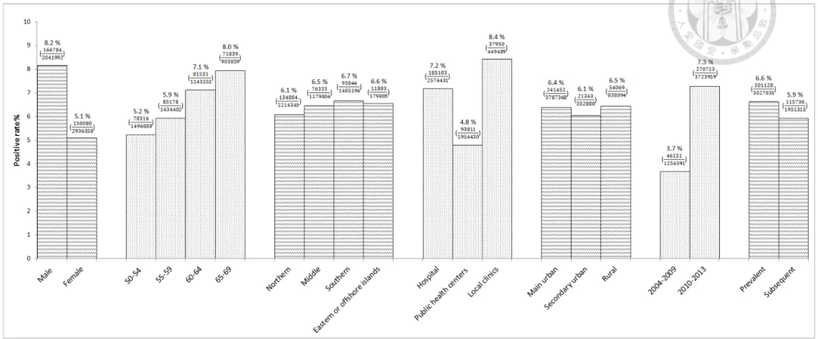
Figure 3-1. Demographics of screening participants in Taiwanese national CRC

screening program from 2004 to 2013 ... 52

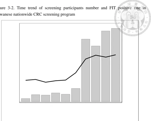
Figure 3-2. Time trend of screening participants number and FIT positive rate in Taiwanese nationwide CRC screening program ... 53

Figure 3-3. Time trend of referral rate and waiting time for colonoscopy in Taiwanese nationwide CRC screening program ... 53

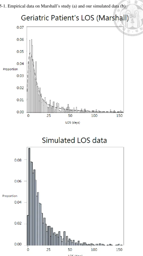
Figure 5-1. Empirical data on Marshall’s study (a) and our simulated data (b) ... 54

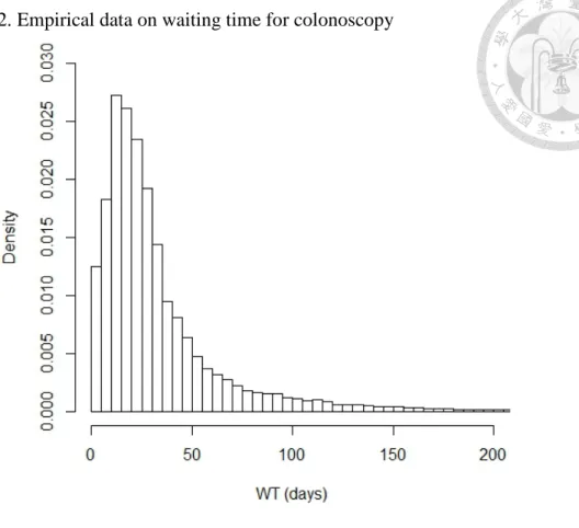
Figure 5-2. Empirical data on waiting time for colonoscopy ... 55

Figure 5-3. Transition probabilities of Coxian two-phase model by risk score ... 56

Figure 5-4. Empirical data on LOS ... 57

Figure 5-5. Fitted three-phase Coxian phase-type distribution for SKH data set... 57

Figure 5-6. Transition probability over time by gender... 58

Figure 5-7. Transition probability over time by age ... 58

(10)

ix

Table

Table 3-1. Demographics of screening participants in Taiwanese national CRC screening program from 2004 to 2013 ... 59 Table 3-2. Descriptive results of attendees, positive rate, referral rate, the distribution of waiting time (WT) ... 60 Table 3-3. Comparison of referral rate and median WT for colonoscopy in inaugural and rolling out period ... 61 Table 3-4. Distributions of discharge types ... 62 Table 5-1. Results for fitting Coxian phase-type distribution to the simulated data on

LOS of Marshall study compared with the original findings ... 63 Table 5-2. Univariate analysis of factors affecting the compliance with colonoscopy and WT for undergoing colonoscopy ... 64 Table 5-3. Model Selection for the hurdle regression model for the possible interaction assessment of putative factors ... 65 Table 5-4. Multivariate analysis on main effect and interaction of factors affecting the non-compliance with colonoscopy ... 66 Table 5-5. Multivariate analysis of main effect and interaction of factors affecting WT for undergoing colonoscopy ... 67 Table 5-6. The estimated results of Coxian phase-type models ... 68

(11)

x

Table 5-7. The expected WT calculated with queue hurdle Coxian two-phase phase-type model ... 69 Table 5-8. Estimated results of queue hurdle one-phase Coxian phase-type model

with the covariate of risk score affecting WT for the referral of colonoscopy ... 69 Table 5-9. Estimated results of queue hurdle two-phase Coxian phase-type model

with the covariate of risk score affecting WT for the referral of colonoscopy ... 70 Table 5-10. Estimated results of fitting Coxian phase-type distribution to SKH data

set ... 72 Table 5-11. The expected LOS in phase i (days) among the three-phase Coxian

Phase-type models ... 72 Table 5-12. The comparison of two 3-phase Coxian models assuming three and two

absorbing rates ... 73 Table 5-13. Model selections for Coxian phase-type model ... 74 Table 5-14. Descriptive results of length of stay (LOS) by gender ... 75 Table 5-15. Estimated results on transition rates and regression coefficients regarding

the effect of gender in two-phase Coxian phase-type model ... 76 Table 5-16. Descriptive results of length of stay (LOS) by age ... 78

(12)

xi

Table 5-17. Estimated results on transition rates and regression coefficients regarding the effect of age in two-phase Coxian phase-type model ... 79 Table 6-1. The estimated results of Coxian phase-type models with three

approaches ... 82

(13)

1

Chapter 1 Introduction

While population-based service screening for colorectal cancer (CRC) with fecal immunological test (FIT) has been demonstrated in reducing mortality in several previous studies^[1][2], a concern is raised as to whether the clinical capacity of colonoscopic examination is sufficient enough to meet enormous burden of referrals with positive result of FIT. The waiting time (WT) for undergoing confirmatory diagnosis would be longer if the capacity is not sufficient and vice versa. Although an organized service screening program has been scheduled by the pre-determined referral date, the WT to undergo colonoscopy is still subject to how the referral system with colonoscopy after screening can be offered. It is therefore interesting to get a better understanding of the distribution of WT for undergoing colonoscopy for each organized service screening. The previous study in Canada has shown the average total WT was around 7.5 months^[3]. However, few studies have been conducted to address whether relevant postulated factors such as demographic features, type of institution, geographic areas, calendar period, and prevalent screen or subsequent screen affect the WT.

After early detection of CRC, it is also very interesting to note that the length of stay (LOS) for hospitalization among patients diagnosed as CRC would become heterogeneous with LOS for early detected and late detected CRCs.

(14)

2

Motivated by the empirical data mentioned above, the use of phase-type distribution may be justified. The phase-type time distributions accounting for multi-phase transitions such as short LOS to long LOS for patients during hospitalization have been used to get a better understanding of the underlying dynamic hidden phases. These thoughts have been executed by the use of Coxain phase-type model (Marshall et al^[4]) to estimate LOS for patients hospitalization. It is well acknowledged that the application of Coxian phase-type is very flexible. For example,

the Coxian phase-type distribution may be used to other scenario such as WT for undergoing colonoscopy while a mass screening for CRC is conducted.

Although the Coxian phase-type model has been used in the queue process, its application to population-based screening may need to be modified on the ground of two major reasons. First, the queue process applied to clinical setting is based on individual-based rather than population-based process. How to connect the arrival process among those who have the uptake of population-based screening for CRC with the WT distribution for colonoscopy is the first consideration. In the queue process, the Coxian phase-type model is a specialized case of hyper-exponential queue model. It is natural to consider whether it can be used for hypo-exponential as the referral of participants with positive test may suffer from the problem of non-compliance. From the methodological viewpoint, how to amend the Coxian phase-type model to

(15)

3

accommodate both hyper-exponential and hypo-exponential models, which may be adequate for modelling data on WT making allowance for the non-referral of undergoing colonoscopy, is a challenging task. To solve this issue, we applied the concept of hurdle model with the Poisson regression model to solve the problem of non-compliance while the WT distribution is considered simultaneously. We therefore integrate the queue process, the hurdle model, and the Coxian phase-type model as a unifying model for modelling the queue for colonoscopy and hospitalization of CRC.

As the WT is regarded as time to event, the first part of purpose of my thesis was to develop by combining the hurdle model, the queue process, the Coxian phase-type model as a unified framework to estimate the median and the percentile of WT and further to assess whether the relevant factors are associated with the WT for undergoing colonoscopy.

The second part of my thesis was to the application of the Coxian phase-type model to elucidate the hidden phase of LOS for hospitalization among patients diagnosed as CRC.

(16)

4

Chapter 2 Literature Review

2.1 Evolution of Coxian phase-type distribution

Over the past few decades, Coxian phase-type distributions have been gradually used to model the skewed survival data. The typical example was to apply the Coxian phase-type distribution to modelling hospital LOS of patients and the patient WT in Accident and Emergency Departments^[5] because the proportion of the elderly population tremendously increased recently, leading to enormous medical expenditures

attributed to hospital treatment. Therefore, Marshall^[4] developed the Coxian Phase-type Cost Model (CP-CM) in 2007 to evaluate how to allocate the limited medical resources

and costs.

A patient’s LOS is considered a reliable indicator for measuring the quantity of resources and has a direct impact on the medical expenditures. In this paper, they introduced some previous methods analyzing patient’ LOS: Mean LOS. LOS data are positively skewed, indicating that the majority had a short stay in the hospital whereas few patients had a long stay. If we use mean LOS to estimate LOS, it is less reliable and inaccurate. To tackle this property, the compartment models with 2 or 3 stages or with the Coxian phase-type distribution were used to consider the positive skewness and heterogeneity of LOS.

(17)

5

To discuss the problem of medical costs under the limited medical resources, it is still worthwhile to review several previous methods used to model health-care costs including (1) two regression models that was to estimate mean hospital charges and the other was to estimate the ratio of the average charge per day; (2) Poisson mixture distributions that considered the heterogeneity of patient populations; (3) queuing theory that used the queueing theory to model patient LOS, and then determined the optimal allocation of hospital resources and costs; (4) survival analysis to estimate the medical care costs by using survival analysis, where patient cost data were recognized as survival times with the Kaplan-Meier estimation and the Cox regression model could be considered;(5) 2-state compartment model that represents the acute care and long-stay care separately. Patients in the same compartment had similar characteristics, but they had dissimilar characteristics and different costs in the distinct compartment.

The recently proposed Coxian phase-type distribution could be interpreted as distinct clinical stages of patients in hospital interpreted by the clinical experts. It is natural to extend the Coxian phase-type distribution to the CP-CM enabling the expected expenditures to be estimated. This new model can solve many problems encountered in the previous methods. The following is pertaining to why the CP-CM is thought of as an appropriate model. Firstly, if we use regression analysis, we need normality and equal variance assumption. However, as the LOS data have the skewed

(18)

6

property and heterogeneity, albeit we can take logarithms of LOS to follow normality assumption, regression analysis still cannot be applicable for coping with the heterogeneity. Secondly, if we use the Poisson mixture distribution, we cannot estimate the transition rate from multi-state phase-type transitions. It will be also subject to over-dispersion. Thirdly, although survival analysis is appropriate for censored data and used for a variety of distributional forms, cost estimates may be biased if survival

exceeds the maximal censoring time. Therefore, it is justified to use the CP-CM to overcome these situations.

2.2 Model structure of the Coxian phase-type distribution

The Coxian phase-type distribution describes the time to absorption of a finite Markov chain in continuous time over the phases {1,2,…,k,k+1}. This Markov chain has one absorbing phase (k+1th) and k transient phases (1,…,k). The process only starts in the first transient phase. If the transition is within transient phase, the parameter of its transition rate is denoted as λ_i. If the process is from transient phase to absorbing phase,

the parameter of its transition rate is symbolized as µ_i. Therefore, given in the ith phase at time t, the probability of patient in the i+1th phase after a short time (Δt) can be

expressed as

P(X(t + Δt) = i + 1 |X(t) = i) = λ_iΔt + o(Δt), for i = 1, … , k − 1

(19)

7

Given in the ith phase at time t, the probability of patient in the absorbing phase after a short time (Δt) can be expressed as

P(X(t + Δt) = k + 1 |X(t) = i) = µ_iΔt + o(Δt), for i = 1, … , k

The probability density function (pdf) of the random time variable T, representing the time until absorption, is given by

f(t) = 𝐩𝐩exp(𝐐𝐐t)𝐪𝐪 (2-1) 𝐩𝐩 = (1 0 0 ⋯ 0)

𝐐𝐐 = �

−(λ1+ µ1) λ1 0 ⋯ 0 0

0 −(λ2+ µ2) λ2 ⋯ 0 0

⋮ ⋮ ⋮ ⋱ ⋮ ⋮

0 0 0 ⋯ 0 −µ_k

�

𝐪𝐪 = (µ1 µ2 ⋯ µk)^T

It comprises the probability defining initial transient phases (p), transition rates restricted to the transient phases (Q) and transition rates from transient phases to the absorbing phase (q).

As mentioned above, due to the different costs of distinct treatment and stages of health-care, the CP-CM was developed to model patient’s medical costs and derive the expected total cost from the moment generating function (MGF). It is assumed that the system has been running long enough to reach steady state and that each phase of the system is operating at maximum capacity. Some random variables are defined. It could be divided into three categories:

(20)

8

(1) Time. The random variable T_i is defined the length of time spent in phase i, and follows exponential distribution with λ_i+ µ_i. Then the MGF of T_i is

MT_i(θ) = ∫ exp (θt)f₀^∞ i(t)dt= _λ^λⁱ^+µⁱ

i+µ_i−θ (2-2) (2) Cost. The cost rates are time homogeneous but phase dependent. So if assuming the cost per subject per time unit z in phase i is ciz, it becomes ci. Then, it defined Dij as the total cost per subject that leaves phase j of the system, given it stayed in phase i. It can easily know that Dij has a linear relationship with T, so the MGF of Dij is

Dij = � c𝛙𝛙T𝛙𝛙 j

𝛙𝛙=i

MD_ij(x) = ∏ _λ ^λ^ψ^+µ^ψ

ψ+µ_ψ−xc_ψ

jψ=i (2-3)

(3) The number of subjects. They defined Zij as the number of subjects who leave the system from phase j, given that they started in phase i. It could be disassembled into the number of subjects initially in phase i multiplied by the probability of leaving the system from phase j, given they started in phase i. Therefore, it follows multinomial

distribution, and the MGF is

Zij = ni× pij

Mz_ij,Z_ij+1,…,Z_ik�tij, tij+1, … , tik� = ∏ �∑ p^k_i=1 ^k_j=i ijexp�tij��ⁿⁱ (2-4)

p_ij = �∏ λj−1 γ γ=i �µj

�∏ λ^j_γ=i _γ+µ_γ� if j ≠ k

(21)

9

p_ij = �∏ λj−1 γ

γ=i �

�∏ λ^j−1_γ=i _γ+µ_γ� if j = k

Finally, if we want to get the total cost defined as T_N for all patients while in the system, we can find that it has a linear relationship with Zij and Dij. Therefore, we can figure out its MGF and get the expected future cost for all subjects in the system.

T_N= � � Z_ijD_ij

k j=i k

i=1

MT_N(x) = ∏ �∑ p^k_i=1 ^k_j=i ijM_D_ij(x)�ⁿⁱ (2-5)

Marshall used the CP-CM model to model patients’ costs and calculated the expected cost of patients in hospital. They found that it is an appropriate model and can provide some useful information to clinicians or hospital managers as their future decisions.

2.3 Semi- and Hidden Markov Process

Continuous-time multistate models are widely used in the natural history of chronic diseases. But if we only can observe the process at discrete time points, we have no information about the times or types of events between observation times. The inference becomes difficult. To overcome this issue, the Markov assumption has been made to imply that the sojourn time in these disease states follows exponential distribution which possess the memoryless property, so that it can limit the transition

(22)

10

rates between these states no longer depend on time since entry into the current state.

However, actually the transition intensities of the process often depend on time since entry into a state that calls semi-Markov process. Therefore, the study conducted by Titman^[6] provides an alternative to alleviate this problem by developing an approach that used the phase-type sojourn time distribution to fit semi-Markov models with panel-observed data. In addition, the approach was extended to data where the observed states were subject to measurement errors.

Panel-observed data are that the observation time periods of each measurement are identical for the same patient. Therefore, given the certain observation time, we can observe types of disease states. It no longer needs Markov assumption. Therefore, the panel-observed data can make the inference become easier.

There were several previous studies which also proposed different ways to fit semi-Markov process: (1) If the observation scheme is sufficiently frequent, the likelihood for a semi-Markov model can be expressed easier. All transitions can be observed, although transition times are interval censored. If the process is a panel data, multiple transitions may occur between observations and we need to use multidimensional integral to obtain the likelihood, which becomes very complicated.

(2) When it comes to multiple transitions mentioned in the previous study, the likelihood function would become complex. If it is a progressive model that means

(23)

11

there is only one possible path of transitions and cannot reverse, computation of the integral may be feasible as the model has a small number of states such as 3 or 4. (3) Nonparametric estimation is possible via self-consistent estimators in progressive model.

(4) Progressive model can be fitted semiparametrically with penalized likelihood. (5) Taking two-state recurrent model for example, as it allows reverse transitions that means it can return to the original state, computation of the likelihood will become more intractable. Regarding evenly spaced observation, a minimum chi-square estimation approach can be used to overcome the problem for this model. (6) Stopping-time resampling has been proposed as a simulation based method of computation. (7) If at least one state in the model has the Markov property, the inference for the panel observed semi-Markov models will be much easier. Because of Markov property, the likelihood for an individual can be factorized into sojourn times of departure from the Markov state. (8) In a two state recurrent disease process with panel observed data, they assumed the existence of latent process was a time homogeneous birth death process and its state space was {0,1,2,…}. If a subject was in state 0, he/she would be considered to be disease free. Other stated were considered ill. Therefore, sojourns in the observable illness state are not exponential and the observable process was a semi-Markov process. However, the computation might become straightforward, if the latent Markov structure of the model allowed the likelihood to be expressed as a hidden

(24)

12

Markov model (HMM).

In many clinical studies, the x_i may be regarded as the measurements of a biomarker or screening test. These measurements may have measurement error so that there is a nonzero probability that the state is misclassified. Instead of observing the x_i

directly, we observe o₁, … , o_n. The misclassification probabilities are defined as P{O(t) = s | X(t) = r} = e_rs. (2-6)

That means at time t, it is exactly in state r, but we observe it is in state s. Based on the misclassification probabilities, e_rs remains constant through time and X(t) is a Markov process, so we know that conditional on the true underlying states, the observed states are independent and the o_i can be modeled by a HMM. To present the likelihood contribution of misclassification for an individual, each transition depends on the

complete history of the process. So for each individual, the matrices were constructed as M1, … , Mn, and Mi is an R × R matrix with (r,s) entry prs(ti−1, ti) × es,o_i with t₀ = 0. It presents the misclassification probability that a subject is in state r at time i-1

and actually reaches in state s at time i, but is misclassified in state oi. Then, the likelihood contribution for an individual can be written as

L = π𝐌𝐌_𝟏𝟏𝐌𝐌_𝟐𝟐… 𝐌𝐌_𝐧𝐧𝟏𝟏 (2-7) where π presents the vector of initial state probabilities and 𝟏𝟏 presents a vector of ones of length R. Covariates affecting the transition rates can be modeled by

(25)

13

µ_rs(t; 𝐲𝐲) = µrs(t)exp (βrsT𝐲𝐲), where y is a vector of explanatory variables. Covariate

effects may also be incorporated into the matrix of misclassification probability by assuming linearity on a logit scale logit(e_rs) = αrsT𝐲𝐲.

To describe a Coxian phase-type distribution, they gave a simple two state (alive,dead) survival model for example, demonstrating how a Coxian phase-type distribution could be applied to the sojourn time distribution of each transient state of a general, multistate, semi-Markov model. Consider a two state survival model X(t) with state {1=alive,2=dead}, for which the transition intensity from alive to dead is time inhomogeneous. For a Coxian phase-type model, the sojourn time in the transient state is assumed to be governed by a latent Markov process X*(t) with k transient phases and one absorbing phase k+1 (=dead). The latent process is progressive, so the movement from transient phase j ∈ {1, … , k} is either to the adjacent phase j+1 or to the absorbing state k+1 as below.

The solid line frame presents the observed state X(t) that we can only observe a subject is either alive or dead. The dashed line frame means the latent state X*(t) that

(26)

14

we cannot observe. At time zero, the process is in phase 1. There are two types of parameters. One is (λ₁, … , λ_k−1), the transition intensities between transient phases and the other is (µ₁, … , µ_k), the transition intensities from the transient phase to the absorbing state. These parameters are constant with time, but intensities are different between phases. It induces time inhomogeneity in the movement between the observable states (from alive to dead).

Consider a semi-Markov process X(t) with state space S={1,…,R}, where R is an absorbing state, and t represents time from entry into the initial state. For each of the

observable states r ∈ S we assume there exists a latent process X*(t) with states r₁, … , r_k but we observe only that the subject is in state r. The state space S* of latent

process X*(t) are

𝐒𝐒^∗ = {1₁, 1₂, … , 1_𝑘𝑘} ∪ {2₁, 2₂, … , 2_𝑘𝑘} ∪ ⋯ ∪ {(R − 1)₁, (R − 1)₂, … , (R − 1)_k} ∪ R ,

its dimension is {k(R-1)+1}. In each observable state, it is not necessary to have the same number of latent states.

The sojourn distribution of each nonabsorbing state r of X(t) is assumed to be a k-phase Coxian phase-type distribution, with parameters λr₁, … , λr_k−1, the rates for movement between phases of state r and µr₁s, … , µr_k−1s, the rates for movement out of state r to state s as follows.

(27)

15

The likelihood can be expressed as (2-7), where for an individual the matrix 𝐌𝐌_𝐢𝐢 become {k(R−1) + 1} × {k(R−1) + 1} with (r, s) entry es,x_iprs(t_(i−1), ti), for s ∈ S*. If s is a phase of the observed state xi, then es,x_i = P{X(t) = xi|X^∗(t) = s} takes the value 1 and 0 otherwise.

To incorporate misclassification error, the process is extended to the hidden semi-Markov model (HSMM). The details of the framework refers to Titman et al^[6].

Suppose the misclassification probability matrix is e as (2-6) and each state in X(t) is phase-type distribution. If the latent process X^∗(t) ∈ {r₁, … , r_k} then X(t)=r for r=1,…,R. So the misclassification probability

er∗_js = P�O(t) = s�X^∗(t) = rj� = P(O(t) = s|X(t) = r) = ers , (2-8) for r,s=1,…,R and j=1,…,k. We can find that they are independent of j. Therefore, the latent Markov process, X*(t), defines X(t) deterministically and O(t) | X(t) is multinomial.

The likelihood contribution from an individual can be calculated as

L = π𝐌𝐌_𝟏𝟏^∗𝐌𝐌_𝟐𝟐^∗… 𝐌𝐌_𝐧𝐧^∗𝟏𝟏, (2-9) where M_i^∗ is a {k(R−1) + 1} × {k(R−1) + 1} matrix with (r*, s*) entry

(28)

16

e_s^∗^∗_,o_ip_r^∗_s^∗(t_(i−1), t_i) , for r*, s* ∈ S*. The difference between the HSMM and

semi-Markov model is that the es,x_i in the semi-Markov case is either 0 or 1, but in the hidden semi-Markov case, the e_rs may lie between 0 and 1 and can be treated as unknown parameters.

To explore the development of bronchiolitis obliterans syndrome (BOS) in post-lung-transplantation patients, they used the HMM and the HSMM to fit the data to identify which model was better. It shows the HMM might be the lack of time

homogeneity, so the HSMM could provide a better fit to the data using the phase-type methodology. Through these methods they were able to better characterize the natural

history of lung function decline after thoracic transplantation.

(29)

17

Chapter 3 Data

I. Compliance with colonoscopy from positive FIT of Taiwan nationwide

colorectal cancer screening program

The Taiwan Nationwide CRC screening by FIT is offered for subjects aged 50 to 69 years. The main purpose was to reduce mortality from CRC through early detection.

Those who had fecal hemoglobin concentration (f-Hb) higher than the cutoff of 20 µg Hb/g of feces were considered as positive and were referred for confirmatory tests by colonoscopy.

All the subjects who had ever attended this nationwide screening program during the period from 2004 to 2013 with positive FIT were enrolled in this study. Those who had f-Hb concentration less than 20 µg Hb/g of feces but with family history were also considered as positive test in this study. Those who underwent screening at unknown place, receiving unknown brand to evaluate test characteristics, or having missing f-Hb value were excluded from the following analysis. A total of 4,978,350 subjects attended CRC screening and 316,864 of them had positive test.

Study variables and definition

Baseline characteristics include gender, age at screening, geographic areas, type of screening units, urbanization levels, calendar periods, and round of screening. Subjects

(30)

18

who were detected as positive case for first-time screening were defined as ‘prevalent screen’ and those who were detected for later screening rounds were defined as

‘subsequent screen’. Besides, calendar periods were divided into two periods. In the inaugural 5 years (2004-2009) of the screening program, screening service was mainly offered at the public health center. From 2010 onward, hospitals and local clinics actively invited people for screening. It was divided into two periods, inaugural period and rolling out period, respectively.

Positive Rate, Referral Rate and Median Waiting Time for Colonoscopy

Total positive rate was 6.36% and positive rates of the corresponding characteristics are shown in Table 3-1 and Figure 3-1. Female and those aged 60 years and younger or screening hold at public health centers and during the period of 2004-2009 had a lower positive rate. The difference of positive rates among geographic areas, urbanization levels and rounds of screening were pretty small. The trend of number of attendees and positive rates are presented in Figure 3-2. A soaring trend of attendees and positive rates were noted at year 2009 and 2010. Chronological changes of positive FIT rate, referral rate, and colonoscopy WT are shown in Table 3-2.

Here, we only considered subjects who underwent colonoscopy within 6 months after being detected as positive case and they would be regarded as ‘successful’ referral.

(31)

19

The referral rate and median WT for colonoscopy among subjects with positive FIT are listed in Table 3-3. Overall referral rate and median WT were 72.78% and 28 days during the inaugural period and those for the rolling out period was 59.42% and 46 days.

During the inaugural period, referral rate within age groups and urbanization levels shows a small difference. Male had slightly higher rate than female. Besides, attendees lived in middle Taiwan, underwent screening at public health centers, or was detected at subsequent screen had higher referral rate, and those lived in eastern Taiwan or offshore islands, underwent screening at hospitals, or was detected at prevalent screen had lower referral rate. In rolling out period, within gender groups, the difference in referral rates became small. Those who aged 65-69, underwent at local clinics, or lived at rural area had lower referral rates and northern Taiwanese had higher rate. The rounds of screening had the same drift in these two periods. Both illustrate subsequent screen had higher referral rate. Subjects in rolling out period had lower referral rate and were needed to wait longer time for colonoscopy especially those undergoing screening at local clinics with the WT of 92 days. However, a special discovery was that screening at hospital during rolling out period would reduce WT for colonoscopy from 51 days to 42days. The time trend of referral rate, medium and third quantile of WT are given in Figure 3-3. A decrease in referral rate and increase in WT was observed during the year from 2009 to 2010.

(32)

20

II. Hospitalization of colorectal cancer patients in Shin Kong Wu Ho-su

Memorial Hospital

Based on the computerized information system of Shin Kong Wu Ho-su Memorial

Hospital (SKH) between 1999 and 2013, patients who had received hospital treatment

and whose International Classification of Diseases (ICD) was recorded as 153 or 154 were enrolled as our study population. There were 178 CRC patients who had ever been

hospitalized in SKH between 1999 and 2013.

Study variables and definition

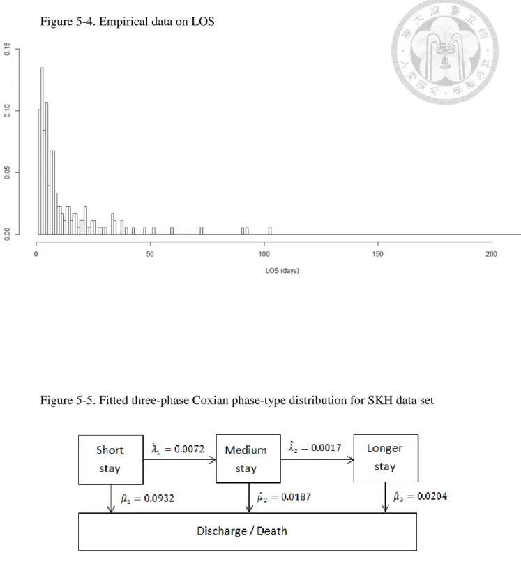
The variables of interest included the patients’ LOS (recorded in days), measured from the day of admission of a patient until they have been discharged. There are six discharge types and their distributions are shown in Table 3-4. The LOS ranges from 1 to 215 days, with a mean of 13.8 days and a median of 7 days.

Baseline characteristics included gender and age at hospitalization. We divided age into those aged below 60, aged between 60 and 74, and aged above 75.

(33)

21

Chapter 4 Methodology

4.1 The hurdle model

Analytical framework of WT for colonoscopy among positive-FIT screenees with the statistical hurdle model is delineated in the following Figure.

(34)

22

To accommodate the non-referral of undergoing colonoscopy (non-complier) and also WT for undergoing colonoscopy among the compliers (see Figure above), we proposed the hurdle model to consider both the non-complier and the WT distribution for the complier. The hurdle part is the application of logistic regression model to identify factors affecting non-compliance with colonoscopy and the progressive part is modelled by the truncated Poisson regression model given the count greater than one to identify factors affecting WT for undergoing colonoscopy.

In the hurdle model assuming there are G subsets determined by relevant covariates (such as age, gender, and so on), yij= 0 representing the j-th screenee of subset i did not undergo colonoscopy and yij = 1 represents the j-th screenee of subset i had underwent colonoscopy for j=1,…,Ni, therefore yi = ∑ yj ij is the number of screenees required for undergoing colonoscopy in subset i and the total number of screenee in subset i is Ni for i=1,…,G. tij is time to undergo colonoscopy of the j-th screenee in subset i, therefore ti = ∑ tj ij represents total WT in subset i. pi is the probability of refusing to undergo colonoscopy (non-complier) estimated with the logistic regression model, and λ_i is the mean arrival rate of receiving colonoscopy estimated with the truncated Poisson regression model which is conditional on at least one screenee undergoing colonoscopy. The hurdle model distribution can be expressed as

(35)

23

(4-1) f(y_i|𝐱𝐱i) = � piN_i−y_i , nonreferral

(1 − pi)^yⁱ_y ^e^−λiti^(λⁱ^tⁱ⁾^yi

i!(1−exp(−λ_it_i)) ,referral where 0 ≤ p_i ≤ 1 ; λ_i, t_i > 0 ; N_i, y_i ≥ 0, xⁱ represents relevant covariates.

The hurdle regression model

The effect of relevant covariates on the non-complier was modelled by using the

following logistic regression model log �_1−p^pⁱ

i� = γ0 + γ1xi1+ γ2xi2+ ⋯ + γkxik (4-2) where γ_j^′s are regression coefficients corresponding to covariates xij′s, and k is the number of covariates considered in each of the model.

The effect of relevant covariates on the WT of the complier was modelled by using the truncated Poisson regression model

log(λ_i) = β₀+ β₁x_i1+ β₂x_i2+ ⋯ + β_kx_ik (4-3) where βj′s are regression coefficients corresponding to covariates xij′s, and k is the number of covariates considered in each of the model.

4.2 Coxian phase-type distributions

The Coxian phase-type distribution describes the time to absorption of a finite Markov chain in continuous time. This Markov chain has one absorbing phase and k transient phases as follows.

(36)

24

The process only starts in the first transient phase. We know (𝐩𝐩, p_k+1) = (1,0,0, ⋯ ,0,0). While LOS data are analyzed, transient phases can represent the severity

of illness and absorbing phase can represent discharge or death, and while WT data are analyzed, transient phases can represent the hidden transition and absorbing phase can represent referral for colonoscopy. When entering the system from the first phase, the subject may move to the second transient phase or the absorbing phase. It is a progressive model and does not allow reverse transitions. As indicated earlier, if the

process is from transient phase to transient phase, the parameter of its transition rate is λ_i. If the process is from transient phase to absorbing phase, the parameter of its

transition rate is µ_i. Therefore, given in the ith phase at time t, the probability of patient

in the i+1th phase after a short time (Δt) is λ_iΔt+o(Δt) for i=1,…,k-1.

P(X(t + Δt) = i + 1 |X(t) = i) = λ_iΔt + o(Δt) (4-4)

Given in the ith phase at time t, the probability of patient in the absorbing phase after a short time (Δt) is µ_iΔt+o(Δt) for i=1,…,k.

P(X(t + Δt) = k + 1 |X(t) = i) = µ_iΔt + o(Δt) (4-5)

(37)

25

Phases {1,…,k} are transient and phase k+1 is absorbing.

The random variable T that is defined as the time to absorption is said to have a Coxian phase-type distribution. The infinitesimal generator for the Markov chain can be

written in block-matrix form as

G = �𝐐𝐐 𝐪𝐪𝟎𝟎 0�

𝐐𝐐 = �

−(λ₁+ µ₁) λ₁ 0 ⋯ 0 0

0 −(λ₂+ µ₂) λ₂ ⋯ 0 0

⋮ ⋮ ⋮ ⋱ ⋮ ⋮

0 0 0 ⋯ 0 −µk

�

𝐪𝐪 = (µ₁ µ₂ ⋯ µ_k)^T

To ensure absorption in a finite time with probability one, it requires that every non-absorbing state is transient, so they block the matrix G and let the matrix Q do not consider the absorbing state. Due to the absorption in a finite time with probability one, the process with Q is an honest Markov process. Therefore, when we want to get solution of the differential equations, we can consider the use of forward and backward Kolmogorov equations. Both sets of equations have the same unique solution to an honest Markov process.

Suppose that initially state i is occupied by X(0)=i, and let pij(t) = P(X(t) = j |X(0) = i).

The forward equations are obtained by the following argument. For Δt>0, pik(t + Δt) = pik(t)[1 + gkkΔt] + ∑ pj≠k ij(t)gjkΔt + o(Δt),

(38)

26

leading to

p_ik^′ (t) = ∑ pj ij(t)gjk.

If we define a matrix P(t), having pij(t) as its (i,j)th element, then

𝐏𝐏^′(𝐭𝐭) = 𝐏𝐏(𝐭𝐭)𝐆𝐆. (4-6)

Now consider the backward equations, it can be obtained by the following argument.

For Δt>0,

pij(t + Δt) = pij(t)[1 + giiΔt] + ∑ pk≠i kj(t)gikΔt + o(Δt),

leading to

p_ij^′(t) = ∑ gk ikpkj(t).

If we define a matrix P(t), having pij(t) as its (i,j)th element, then

𝐏𝐏^′(𝐭𝐭) = 𝐆𝐆𝐏𝐏(𝐭𝐭). (4-7)

The (4-6) and (4-7) with initial condition 𝐏𝐏(𝟎𝟎) = 𝐈𝐈 have the formal solution

𝐏𝐏(𝐭𝐭) = exp(𝐆𝐆t) (4-8) = ∑^∞𝑛𝑛=0𝐆𝐆^{n t}_n!ⁿ (4-9)

When G is a finite matrix, that is when the number of states of the process is finite, the series (4-9) is convergent and (4-8) is the unique solution of both forward and backward equations.

If we assume the process has 3 transient phases and one absorbing phase (4^th phase). The transition matrix is expressed as

(39)

27

G = �

−(λ₁+ µ₁) λ₁ 0 µ₁ 0 −(λ2+ µ2) λ2 µ2

0 0 −µ₃ µ₃

0 0 0 0

�

We can obtain its transition probability by (4-8) or using the stochastic integral as follows.

P12(t) = λ₁[e^−(λ¹^+µ¹^)t− e^−(λ²^+µ²^)t] (λ2+ µ2) − (λ1+ µ1)

P13(t) = λ₁λ₂ µ₃− (λ₂+ µ₂) �

e^−(λ¹^+µ¹^)t− e^−(λ²^+µ²^)t (λ₂+ µ₂) − (λ₁+ µ₁) −

e^−(λ¹^+µ¹^)t− e^−µ³^t µ₃− (λ₁+ µ₁) �

P23(t) =λ₂[e^−(λ²^+µ²^)t− e^−µ³^t] µ3− (λ2+ µ2)

P24(t) = 1 − e^−(λ²^+µ²^)t−e^−(λ²^+µ²^)t− e^−µ³^t µ3− (λ2+ µ2)

P₃₄(t) = 1 − e^−µ³^t

P14(t) = 1 − P11(t) − P12(t) − P13(t) = 1 − e^−(λ¹^+µ¹^)t− P12(t) − P13(t) (4-10) If the random variable T_i represents their LOS/WT in phase i, where T_i~exp (λ_i+ µ_i),

the MGF for the length of time a patient spends in phase i is given by M_T_i(θ) = λ_i+ µ_i

λ_i+ µ_i− θ Therefore, the expected LOS/WT in phase i, determined by

E[Ti] = 1 λi+ µi

(40)

28

And the marginal mean LOS/WT in the system can be obtained by E[T] = � t dP^∞ 14(t)

0

4.3 Queue Hurdle Coxian Phase-type model

In order to take into account the arrival rate of eligible screenees, non-compliance with colonoscopy and the WT for undergoing colonoscopy simultaneously, we used the Poisson distribution to model arrival rate and apply Coxian Phase-type distribution to non-hurdle part of hurdle model. As a result, we developed the Queue Hurdle Coxian Phase-type model as follows.

In the Queue Hurdle Coxian Phase-type model, it has three components: (1)

Poisson Queue process, ν is the arrival rate of eligible screenees per person-days, y_i = 1 is positive FIT and y_i = 0 is negative FIT, the Poisson distribution can be

displayed as

(41)

29

(4-11) f(y_i) =^{exp (−νt}_yⁱ^)(νtⁱ⁾^yi

i! , ν > 0; i = 1, … , n ,

(2) Probability of non-compliance with colonoscopy, say p, (3) Coxian Phase-type distribution, its pdf is the derivative of the transition probabilities derived from (4-8), therefore the Queue Hurdle Coxian Phase-type distribution can be expressed as

f(t₁, t₂) = � e^−νt¹ , FIT (−) e^−νt¹(νt1) × p , FIT (+) but nonrefer

e^−νt¹(νt1) × (1 − p) × fC(t2) , FIT (+) and referral

where t₁ is the arrival time from invitation date to screening date, t₂ is the WT for undergoing colonoscopic exam, and f_C(t₂) is the p.d.f of Coxian Phase-type distribution based on the derivative of the transition probabilities derived from (4-8).

(42)

30

Chapter 5 Results

I. Computer Simulation for Estimating Parameters

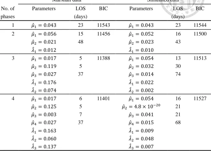
To test if the Coxian phase-type model can be simulated by directly using a mixture of Poisson process, we fit the continuous positively skewed data on which the research conducted by Marshall^[4] was based after simulating their tabular data on LOS of the geriatric patients. As the most adequate model was fitted by a 3-phase Coxian phase-type distribution we simulated the data by a 3-state mixture Poisson process with

the probability density function expressed as follows.

f(t) = π1× θ1e^−θ¹^t+ π2× θ2e^−θ²^t+ π3× θ3e^−θ³^t, (π1+ π2+ π3 = 1)

We set π₁ = 0.46 , π₂ = 0.40 , π₃ = 0.14 and θ₁ = 0.07 , θ₂ = 0.05 , θ₃ = 0.02 . The data set in Marshall’s study indicated the LOS ranged from 0 to 350 days, with a mean of 23 days and a median of 12 days. The simulated data shows the LOS ranged from 0 to 358 days, with 23 days and a median of 14 days (Figure 5-1), which was very close to their original empirical findings.

The Coxian phase-type distribution was fitted to the simulated data by using SAS software. SAS implements an optimization function with the method of maximum likelihood estimation (MLE) given the formulation of the log-likelihood function for different kinds of phase-type distribution. We used the Newton-Raphson algorithm and the minimum Bayesian information criterion (BIC) to decide the most parsimonious

(43)

31

model. In Table 5-1, the estimated parameters in the one or two phase Coxian phase-type model were close between the original results and our simulated data.

However, when the number of phase increased there was a larger discrepancy. The results of simulation suggest while the hidden phases increased the heterogeneity across different phases could not be captured by a mixture of Poisson process.

II. Compliance with colonoscopy from positive FIT of Taiwan nationwide

colorectal cancer screening program

Univariate Analyses and Multivariate Analyses for the Hurdle model

In order to identify factors associated the non-compliance for colonoscopy and those affecting WT for undergoing colonoscopy, we used the hurdle model to deal with these two problems simultaneously.

The hurdle part is to identify which factors might influence subject not to take colonoscopic exam and the non-hurdle part is to identify which factors would affect WT for colonoscopy among attendees complying with colonoscopy. As shown in Table 5-2, the effects of gender on both parts of model were lacking of statistical significance.

Compared with the age group of 50-54, the older age groups had higher odds of refusing to receive colonoscopy whereas the complier after they underwent colonoscopy exam, the effect of age on WT became not statistically significant. In geographic area,

(44)

32

those residing in Eastern Taiwan or offshore islands had the highest odds of non-compliance and had the longest WT for colonoscopy if they actually received colonoscopy exam; those dwelling in Northern Taiwan had the lowest odds of non-compliance and had the shorter WT for colonoscopy than those dwelling in Southern or Eastern Taiwan or offshore islands. Those who attended screening at public health centers had the lowest odds of non-compliance and had the short WT for colonoscopy; those who attended screening at local clinic had the highest odds of non-compliance and had the longest WT for colonoscopy. Attendees living in secondary urban or undergoing screening at inaugural period or being detected at subsequent screening had the lowest odds of non-compliance and had the shortest WT for colonoscopy.

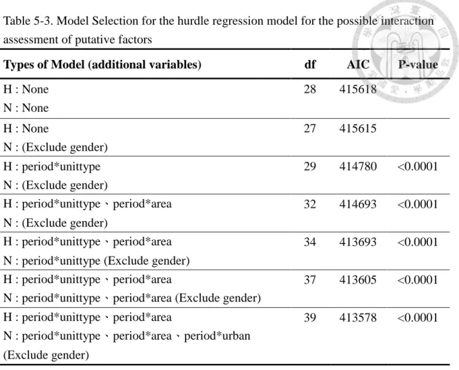
Before fitting the multivariate model, the model selection was done and shown in Table 5-3. Because the change in the structure of screening program during the year from 2009 to 2010 might results in heterogeneity between the inaugural period and rolling out period, we evaluated the interaction between factors and periods of screening program. The results of model selection reveal that the hurdle part included seven baseline characteristics and interaction of periods of screening program between geographic areas and type of screening units, and the non-hurdle part contained six baseline characteristics (excluding gender effect) and interaction of periods of screening

(45)

33

program between geographic areas, type of screening units and urbanization levels. As presented in Table 5-4, multivariate analysis in hurdle part found female, older people, those who lived less urbanized area and those were detected at prevalent screen had higher chance of not complying with colonoscopy. During inaugural period, attendees of eastern Taiwanese or offshore islands had a highest odds of not complying with colonoscopy (OR: 1.51, 95% CI: 1.36-1.66) compared with the northern attendee, but in rolling out period, middle Taiwanese had the highest odds of not complying with colonoscopy (OR: 1.08 95% CI: 1.06-1.10). Although screening at public health centers had the lowest odds in both periods, screening at hospital had the highest odds (OR:

2.54, 95% CI: 2.39-2.69) in inaugural period but decreased during the rolling out period (OR: 1.08, 95% CI 1.06-1.10) and screening at local clinic (OR: 1.79, 95% CI:

1.74-1.84) had the highest odds in rolling out period. When taking the non-hurdle part into account, the results presented in Table 5-5 show attendees who aged between 65 and 69 years had the longest WT for colonoscopy if they actually complied with colonoscopy, but three other age groups had not much difference. Those detected at subsequent screen had shorter WT for colonoscopy than prevalent screen. During inaugural period, attendees living in middle Taiwan (RR: 1.14, 95% CI: 1.07-1.20) or main urban or undergoing screening at public health centers (RR: 1.22, 95% CI:

0.99-1.46) had the shortest WT for colonoscopy. During the rolling out period, those

(46)

34

who lived in middle Taiwan (RR: 1.13, 95% CI: 1.09-1.16) or secondary urban area (RR:

1.07, 95% CI: 1.06-1.09) or undergoing screening at hospital (RR: 1.14, 95% CI:

1.12-1.15) had the shortest WT. It indicates the similar trend in geographic areas in both periods, and the estimates of RR of northern people increased from 1.03 to 1.12.

Queue Hurdle Coxian Phase-type model

As we had already known there was heterogeneity between the inaugural period (2004-2009) and the rolling out period (2010-2013), so we analyzed these two separately. In the current thesis, we only considered the modelling with the Coxian phase-type model using the data on the inaugural period. The continuous data are positively skewed with a long tail, representing those few attendees who had not received colonoscopic exam for an extremely long WT (Figure 5-2) that justifies the WT had better be modelled by the Coxian phase-type distribution. To decide the most appropriate model, we still used the minimum BIC to determine. In Table 5-6, we found the Queue hurdle 2-phase Coxian phase-type model was the most suitable model due to minimum BIC score and could be classified as short waiting (step-by-step) phase and long waiting (shilly-shally) phase. It can be clearly seen that the 3-phase Coxian phase-type model had higher BIC value and also showed the identifiability problem between the referral rate from the moderate waiting phase (µ₂) and the transition rate