科技部補助專題研究計畫報告
一個基於圖形處理器(GPU)的即時微震監測平台(第3年)
報 告 類 別 : 成果報告 計 畫 類 別 : 個別型計畫 計 畫 編 號 : MOST 106-2628-M-006-001-MY3 執 行 期 間 : 108年08月01日至109年07月31日 執 行 單 位 : 國立成功大學地球科學系(所) 計 畫 主 持 人 : 李恩瑞 計畫參與人員: 學士級-專任助理:吳秉芬 碩士班研究生-兼任助理:何宗璟 碩士班研究生-兼任助理:蕭欣宜 碩士班研究生-兼任助理:廖勿渝 碩士班研究生-兼任助理:許沛然 碩士班研究生-兼任助理:康倫愷 碩士班研究生-兼任助理:黃籍億 碩士班研究生-兼任助理:葉儒 碩士班研究生-兼任助理:林容辰 大專生-兼任助理:何立新 大專生-兼任助理:黃籍億 大專生-兼任助理:張家瑋本研究具有政策應用參考價值:□否 ■是,建議提供機關交通部
(勾選「是」者,請列舉建議可提供施政參考之業務主管機關)
本研究具影響公共利益之重大發現:■否 □是
中 文 摘 要 : 對地震形成過程的物理機制(如:地震成核、地震觸發、震後變形)完 整的前震和餘震目錄,將對其分析扮演著關鍵角色。快速準確的地 震檢測和定位算法,可提供及時地震活動信息,從而有助於我們理 解地震的物理機制和地震危險性評估。我們利用圖形處理單元 (GPU)加速並自動化微震監測,並將演算法命名GAMMA,用於精確和 近實時的地震檢測和定位。 GAMMA利用基於反投影的方法自動檢測 潛在的地震,然後使用模板匹配算法在連續記錄中搜索小地震時 ,選擇地震的波形作為模板。 GPU的使用大大加快了計算速度,並 使GAMMA能夠近及時地震監測。我們已成功將GAMMA應用於2019年在 加州的Ridgecrest地震序列。 GAMMA探測到的地震數量是南加州地 震中心目錄中記錄的21倍以上。由GAMMA確定的更完整的目錄可能會 提供重要信息,以增進我們對斷層物理機制的理解,並為各種類型 的研究(包括動態破裂模擬和地殼變形模型)提供有用的控制條件 。 中 文 關 鍵 詞 : 前震、餘震、圖形處理單元、微震監測
英 文 摘 要 : Foreshocks and/or aftershocks play critical roles in improving our understanding of the processes of faulting, such as nucleation of earthquakes, earthquake triggering, and postseismic deformation. A rapid and accurate
earthquake detection and location algorithm can provide timely information of seismic activities, thereby
benefitting our understanding of physical mechanisms of faulting and seismic hazard assessment. We have developed a graphic processing unit (GPU)-accelerated automatic
microseismic monitoring algorithm (GAMMA) for accurate and near real-time detection and location of earthquakes. GAMMA utilizes methods based on backprojection to automatically detect potential earthquakes, and then the waveforms of qualified earthquakes are selected as templates when searching for small earthquakes in continuous recordings using the template-matching algorithm. The use of GPUs has substantially accelerated the calculations and has made GAMMA capable of (near-)real-time earthquake monitoring. We have successfully applied GAMMA to the 2019 Ridgecrest earthquake sequence in southern California. The number of earthquakes detected by GAMMA is more than 21 times that documented in the regional catalog. The more complete
catalog determined by GAMMA may provide crucial information for improving our understanding of the physical mechanisms of faulting and also supply useful constraints for a
variety of types of studies, including dynamic rupture simulations and crustal deformation modeling.
英 文 關 鍵 詞 : foreshock, aftershock, graphic processing unit (GPU), microseismic monitoring
GPU-accelerated Automatic Microseismic Monitoring Algorithm (GAMMA) and its Application to the 2019 Ridgecrest Earthquake Sequence
Abstract
Foreshocks and/or aftershocks play critical roles in improving our understanding of the processes of faulting, such as nucleation of earthquakes, earthquake triggering, and post-seismic deformation. A rapid and accurate earthquake detection and location algorithm can provide timely information of seismic activities, thereby benefitting our
understanding of physical mechanisms of faulting and seismic hazard assessment. We have developed a GPU-accelerated Automatic Microseismic Monitoring Algorithm (GAMMA) for accurate and near real-time detection and location of earthquakes. GAMMA utilizes methods based on back-projection to automatically detect potential earthquakes and then the waveforms of qualified earthquakes are selected as templates when searching for small earthquakes in continuous recordings using the template-matching algorithm (TMA). The use of GPUs has substantially accelerated the
calculations and has made GAMMA capable of (near) real-time earthquake monitoring. We have successfully applied GAMMA to the 2019 Ridgecrest Earthquake Sequence in Southern California. The number of earthquakes detected by GAMMA is more than 21 times of that documented in the regional catalog. The more complete catalog determined by GAMMA may provide crucial information for improving our understanding of the physical mechanisms of faulting and also supply useful constraints for a variety types of studies, including dynamic rupture simulations and crustal deformation modeling.
1. Introduction
The 5 July 2019 Ridgecrest earthquake (Mw 7.1) was the most powerful earthquake in
California after the 1999 Mw 7.1 Hector Mine earthquake. It occurred on the NW-SE
trending Little Lake Fault Zone (LLFZ), which lies at the northern extension of the Eastern California Shear Zone (ECSZ). It was followed by ~3,000 detected aftershocks with magnitudes ranging approximately 2-5.5 Mw within a couple of days. The
hypocenters of the aftershocks extended ~50 km along the LLFZ. It has been estimated that the total number of aftershocks in the six months following the mainshock will be ~34,000 (Wigglesworth, 2019). The Ridgecrest mainshock was preceded by an Mw 6.4
foreshock on a previously unnoticed NE-SW trending fault less than two days ago. The Mw 6.4 foreshock was itself preceded by several smaller foreshocks and followed by an
unusually large number of detected aftershocks (~1,400) with magnitudes ranging approximately 2-5.4 Mw (Croft & Goyette, 2019) before the occurrence of the Mw 7.1
mainshock. The hypocenters of the aftershocks following the Mw 6.4 foreshock revealed
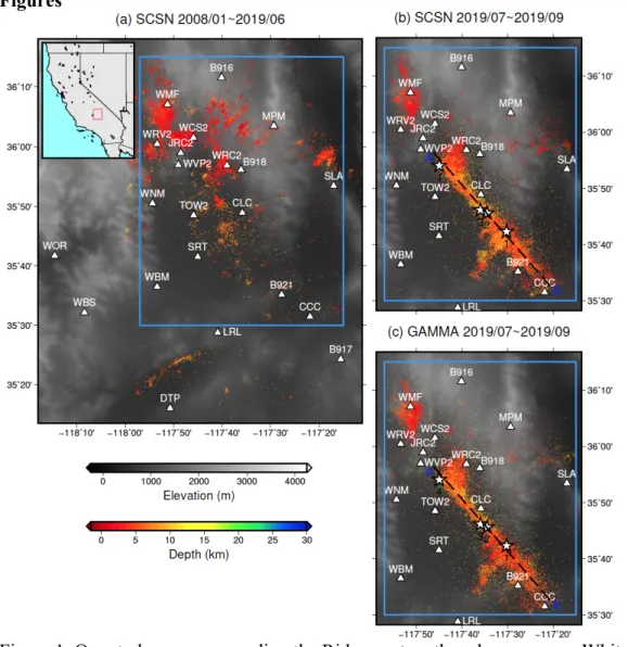
the previously unspecified NE-SW trending fault zone that is conjugate to the NW-SE trending LLFZ (Figure 1).
In-depth studies of the Ridgecrest foreshock-mainshock-aftershock sequence rely upon robust detection and accurate (re)location of the foreshocks and the aftershocks, which are particularly challenging considering their small magnitudes, therefore relatively poor signal-to-noise ratios (SNR) of their waveform recordings in general, and also the
interferences both with the major quakes and among themselves. In this study, we present a GPU-accelerated automatic microseismic monitoring algorithm (GAMMA), which combines our previous GPU implementation of the template-matching algorithm (TMA) (Mu et al., 2017) with a GPU-accelerated back-projection algorithm and an automatic phase-picking code based on the deep convolutional “attention U-Net” (e.g., Ronneberger et al., 2015; Çiçek et al., 2016; Liao, 2019), for rapid and fully automated detection and (re)location of the foreshocks and the aftershocks. Each individual technology used in GAMMA has been documented in different publications before. However, to the best of our knowledge, the adoption of “attention U-net” (i.e., the deep convolutional U-net incorporated with “attention gates”) for seismic phase picking is new and the integration of these different technologies in a unified, automatic, and GPU-accelerated workflow for earthquake detection and location is new.
The initial application of our GAMMA code on the continuous waveform recordings at 22 three-component broadband, strong-motion, and short-period seismic stations surrounding the Ridgecrest sequence (Figure 1) gave highly promising results. It took less than 3 hours to process one day of the continuous waveform recordings at all the seismic stations using a single server equipped with 8 GeForce RTX 1080 Ti GPUs. The total number of foreshock/aftershock events detected by GAMMA so far is over 21 times of that reported in the Southern California Seismic Network (SCSN) catalog. At first glance, the number of events detected by GAMMA may appear to be unusually large. It is therefore of particular importance for us to provide a detailed account of the
methodology and implementation of GAMMA in order to convince readers that our detected events are indeed real earthquakes, rather than false detections caused by incorrect methods and/or faulty implementations. In addition to providing a more complete earthquake catalog, the hypocenters and origin times determined using GAMMA show intriguing spatial and temporal patterns, which may help to reveal previously unmapped, small-scale fault zone structures and potential interactions among them.
2. Instruments and Data Availability
The availability of the catalog for the Ridgecrest sequence obtained using GAMMA is provided in section 6 “Data and Resources” of this letter. Here we provide a very brief introduction about the instrumentation used in our study, which consists of the seismic stations of the SCSN.
The SCSN is a cooperative seismic network part of the California Integrated Seismic Network (CISN). It was composed of ~250 short-period instruments through much of 1980’s and 1990’s and some of those instruments are still in-use today. It was gradually supplemented with digital stations with broadband and strong-motion sensors in the 1990’s and 2000’s. Today, it consists of over ~200 three-component, broadband and strong-motion stations and the onsite clock time is calibrated using the Global Positioning System (GPS) (Hutton et al., 2010). Figure 1 shows our study area and the locations of the 22 SCSN stations used for the detection and location of the events in the Ridgecrest
prefer stations with three-component, continuous recordings and we prefer broadband instruments to short-period and strong-motion instruments. The details of the stations can be found on the websites listed in section 6 of this letter. The seismic waveform
recordings used in this study were downloaded using the Seismogram Transfer Program (STP) released by the Southern California Earthquake Data Center (SCEDC) (section 6).
3. Methodology
A routine task of many seismic networks, such as SCSN, is the detection and location of regional earthquakes. Many of the conventional techniques adopted by seismic networks rely upon the correct identification of the onset time of P- and/or S-wave arrivals using triggering algorithms, such as the ratio between short-term and long-term average amplitudes (STA/LTA) of the continuous waveform recordings. Calculations of such triggering algorithms can be carried out using conventional desktop computers with almost negligible amount of computing time. When combined with real-time telemetered seismic data feeds from multiple stations, these conventional techniques have enabled (near) real-time earthquake detection and location. However, the performance of conventional triggering algorithms can deteriorate, sometimes significantly, for earthquakes lacking easily identifiable P- or S-wave onsets, which is typical for small earthquakes with poor waveform SNR and non-tectonic events such as landslides (e.g., Kao et al., 2012; Lee et al., 2019), volcanic tremors (e.g., Langet et al., 2014) and human-induced seismicity (e.g., van der Baan & Calixto, 2017). To remedy the drawbacks of conventional triggering-based techniques, new algorithms have been proposed and tested and among them the template-matching algorithm (TMA) (e.g., Gibbons and Ringdal, 2006; Shelly et al., 2007; Peng and Zhao, 2009; Peng and Gomberg, 2010) is a highly promising candidate.
The TMA is based upon computing the normalized cross-correlation coefficients (NCC) between a large collection of pre-selected template waveforms, which were generated by previously identified earthquakes and recorded at a set of seismic stations, and the corresponding continuous waveform recordings at the same set of stations. If the NCC values at multiple stations exceed a pre-specified threshold value, a new event is
detected. Because the TMA utilizes the shape of the entire waveform train for detection, it is much more robust than conventional triggering-based algorithms such as STA/LTA, especially for small and/or non-tectonic events with no clearly identifiable P- or S-wave onsets. Recent applications of TMA in Southern California have revealed a large number of previously undetected “hidden” earthquakes (Ross et al., 2019), which were missing from the SCSN catalog constructed using conventional detection techniques.
We are facing two major challenges when implementing TMA-based techniques in routine earthquake detection and location. First, because the NCC must be computed for a large number of template waveforms (sometimes up to tens of thousands) at time windows moving along the continuous recordings of a potentially large number of channels, the computational cost of the TMA is much higher than conventional
algorithms based on STA/LTA, which makes it challenging to adopt TMA in (near) real-time applications. Second, because the fundamental principle behind the TMA-based
detection algorithm is that earthquakes with similar locations and mechanisms tend to produce similar waveforms at the same stations, the performance of TMA-based techniques relies heavily upon the completeness of the pre-constructed template waveform database. How to construct the template waveform database in a systematic, self-consistent and automatic workflow is still a major challenge.
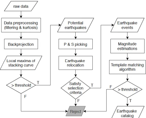
To address the first challenge associated with TMA’s high computational cost, we developed a GPU-accelerated TMA code “cuNCC” (Mu et al., 2017), which achieved a speedup factor of nearly three orders of magnitude on a commodity GPU card (Nvidia GTX 980) with respect to a sequential CPU code running on the Intel Xeon E7-8867 V4 processor, thereby opening up the possibilities of adopting TMA in (near) real-time applications. In this study, we address the second challenge associated with the construction of the template waveform database. We propose a systematic workflow centered on a GPU-accelerated back-projection algorithm (Figure 2) to automatically assimilate waveforms with high SNR from distinct source locations into the template waveform database. To further improve the accuracy of the origin time and hypocenter locations of the “template sources” (i.e., those sources that generate the template waveforms), we incorporated an automatic phase-picking code based on the deep
convolutional “attention U-Net” (e.g., Oktay et al., 2018) into our workflow and adopted a 3D seismic velocity model, CVM-S4.26 (Lee et al., 2014; Chen & Lee, 2015; Lee & Chen, 2016), for the Ridgecrest area under study (Figure 1).
3.1. Data preparation
We divided the continuous recording at each component of the station (Figure 1) into 80-minute-long segments centered on the hour with a 10-minute overlap between
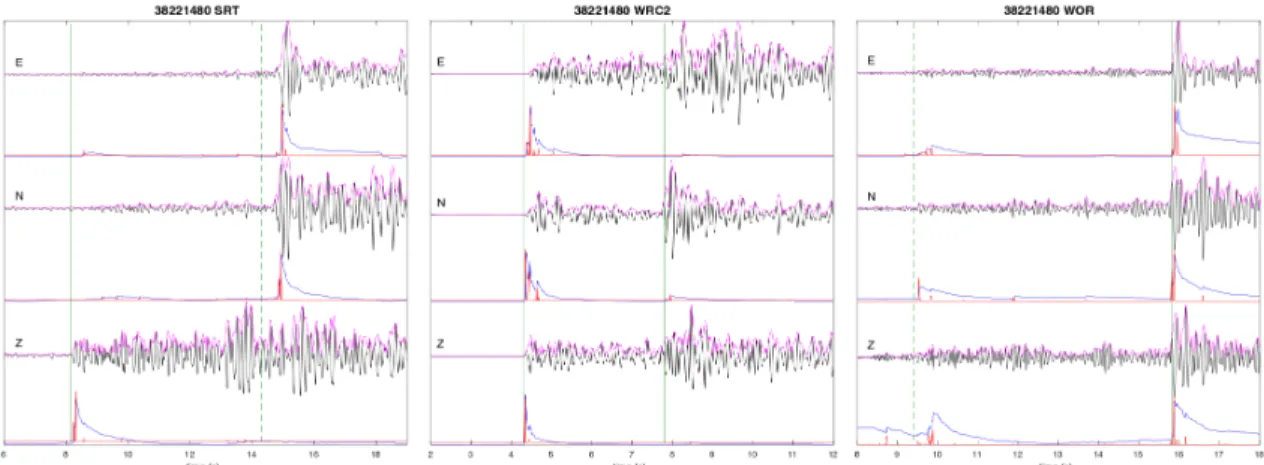
neighboring segments. The mean and the linear trend of each segment were removed and a taper was applied to each end of the segment. Each segment was then band-pass filtered from 3 to 12 Hz and decimated to 25 samples per second. The kurtosis function, which is the 4th standardized moment of a signal, was then computed for a 3-second-long time
window sliding from the beginning of the hour to 2 minutes after the end of the hour. The kurtosis function tends to reach local maxima around the P- and/or S-wave onset time (Figure 3); however, the widths of the peaks can be relatively broad (Langet et al., 2014), which may introduce errors into the estimated source location and origin time after back-projection. To make the peaks narrower and more centered on the P- and/or S-wave onset time, we calculated the positive time derivative of the kurtosis function, which equals to the time derivative of the kurtosis when the time derivative is positive and zero when the time derivative is negative (Langet et al., 2014). Figure 3 shows examples of the kurtosis and its positive time derivative function for an earthquake (SCSN event ID: 38221480) in our study area.
3.2. Back-projection for template source detection
The positive time derivatives of the kurtosis functions from multiple components of all the stations were then used as the input to our GPU-accelerated back-projection code.
source, is an effective technique for estimating source locations and origin time (Langet et al., 2014; Tan et al., 2019) and has been successfully applied to locate not only earthquakes but also non-tectonic events, such as non-volcanic tremor (e.g., Wech & Creager, 2008) and landslides (e.g., Kao et al., 2012; Lee et al., 2019).
In our implementation, the positive time derivatives of the kurtosis functions obtained from the three components of all the stations were shifted according to a pre-computed travel-time table and then stacked with equal weights across all components of all stations. The travel-time table was computed for both P- and S-wave from every station location to all the potential source locations, which consist of the 145,692 grid points of a uniform mesh covering our study volume (Figure 1) with 0.01° lateral and 1-km vertical grid spacing, using Simul2000 (Thurber & Eberhart-Phillips, 1999) and the 3D seismic velocity model CVM-S4.26. This 3D seismic velocity model was obtained from full-3D seismic waveform tomography using both ambient-noise Green’s functions and regional earthquake seismograms (Lee et al., 2014). It includes 3D crustal heterogeneities that account for the sedimentary basins, such as the Indian Wells Valley (China Lake) in our study area (Lee & Chen, 2016).
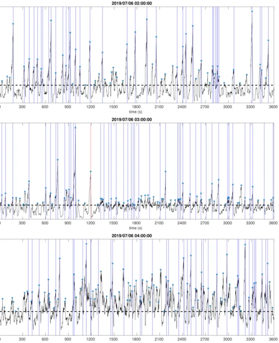
Figure 4 shows examples of our one-hour-long, stacked back-projections at one grid point (i.e., a potential source location), which have many local maxima corresponding to the origin times of potential earthquakes. Local maxima with amplitudes larger than a pre-specified threshold were selected as potential template sources. In our study, we used the origin times of small earthquakes (ML < 1.0) from 1 July 2019 to 3 July 2019 in the
SCSN catalog to determine the threshold value. We set the threshold at a value such that the differences in the origin times of those small earthquakes between our results and those in the SCSN catalog were minimized.
Because for every potential source location the positive time derivatives of the kurtosis functions from the 3 components of every station must be shifted according to both P- and S-wave travel-times and then stacked, considering the total number of potential source locations, the back-projection process can be computationally intensive. However, the calculations for different potential source locations are independent of one another. To fully exploit this inherent parallelism, we have developed a GPU-accelerated version of the back-projection code, which has achieved a speedup factor of ~40 times on a single Nvidia 1080Ti GPU with respect to the sequential CPU code. For this study, it took less than 3 minutes of wall-time to back-project and stack the one-hour-long segments from all components of all stations for all potential source locations. We are not aware of any other GPU back-projection code that can achieve a similar or better speedup factor.
3.3. Template source inversion 3.3.1. Automatic phase picking
To improve the accuracy of origin times and hypocenter locations of the potential template sources identified in our back-projection process, we need to further refine the P- and/or S-wave arrival-time picks. In this study, we have developed an “attention
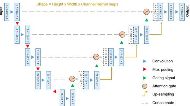
U-Net” algorithm (Figure 5) for phase picking (Liao, 2019) and we have validated the results with those obtained using the more conventional phase picker based on the Akaike Information Criterion (AIC) (e.g., Maeda, 1985; Zhang et al., 2003).
The U-Net (e.g., Ronneberger et al., 2015; Çiçek et al., 2016; Zhang et al., 2018; Zhou et al., 2018) is a special type of deep convolutional neural network (CNN), which has been used widely in various image-related machine-learning studies. It addresses the missing-feature problem in conventional deep CNN by implementing channel-wise
skip-connections on its encoder-decoder structures. The seismograms recorded at
3-component stations can be treated as 3-channel 1-D images, which allows U-Net or other types of deep CNN to be adopted for automatic seismic phase picking (e.g., Ross et al., 2018a; Zhu & Beroza, 2018; Zhu et al., 2019).
To reduce the impact of random noise, the interferences from unrelated seismic events and other unlabeled signals on the training process, we have adopted the “attention U-Net” (e.g., Oktay et al., 2018) in this study. The attention U-Net integrates attention gates (Figure 5) into the standard U-Net. The attention gates adjust the training weights of signals for skip-connection by integrating low-level and high-level feature maps. Such soft attention mechanisms are computationally more economical than reinforcement learning, while providing similar functionalities. In our study, we have found that the attention U-Net is particularly effective in picking S-waves. The manually picked phases, which are used as labels in the training process, are usually more consistent for P-waves than for S-waves, because S-waves are often mixed with other types of signals, such as P-coda, converted waves, surface waves. The attention U-Net avoids training uncertain features and reduces the impact from other signals (Liao, 2019).
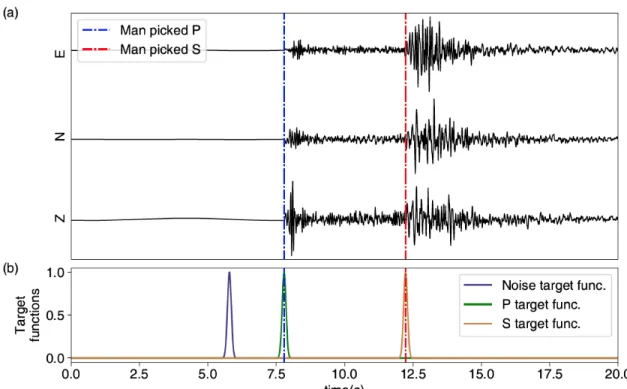
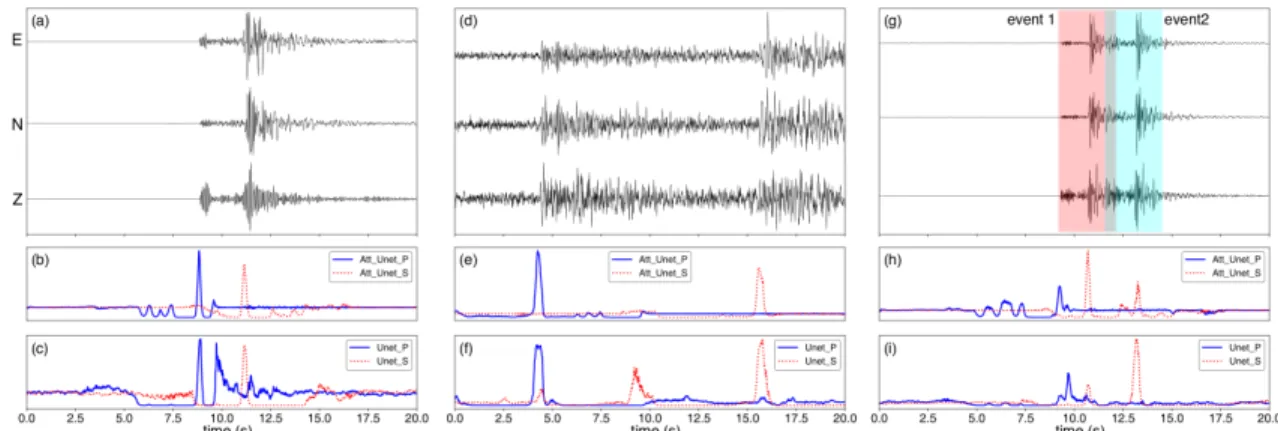
Figure 6 shows examples of the “target functions” used in the training process and Figure 7 shows comparisons of the predictions made using our attention U-Net and the standard U-Net after the training process was completed. The outputs of our neural networks were probabilities of the P- and S-wave onsets as functions of time, with the option of the probability for a noise or “other” phase. The target functions were constructed by
centering Gaussian probability distributions on the manual picks (Figure 6) and were then used as labels during the training process. We use the recordings of earthquakes occurred during January 1, 2008 to June 30, 2019 in our study area (Figure 1a) at the selected stations for training and model validation of our deep learning method. For data quality control, we reject the recordings with SNR of P or S less than 5. The predictions made using the standard U-Net can have strong secondary peaks (Figure 7c and f), while those secondary peaks were mostly removed on the predictions made using our attention U-Net (Figure 7b and e). When locating the template sources in the Ridgecrest sequence, we used 85,774 P and S picks for training/validation and 31,471 picks for testing. The P and S picks with residuals less than 0.15s are considered as true positive picks. The prediction precision of our attention U-net for P and S waves is 98% and 97%, respectively. In general, we have found that the predictions made using our attention U-Net are more consistent with human choices than those made using the standard U-Net. For P waves, the prediction precision of our attention U-net is similar to that of the standard U-net
(~96%), while for S waves, the prediction precision of our attention U-net is substantially better than that of the standard U-net (~85%) (e.g., Zhu & Beroza, 2018).
When seismicity is high, multiple earthquakes can occur at very close time, which may lead to overlaps on seismic waveform recordings. When the waveforms (e.g. P and S waves) from different earthquakes are mixed (e.g. Figure 7g), it is highly challenging to make the correct P and S picks for each individual earthquake, even with manual checks. The predicted P and S arrivals based on the initial source location obtained during our back-projection stage provide initial references for P and S phase selections. We therefore select the local maxima, rather than the global maxima, of the P and S probability functions within ±1.5s of the predicted P and S arrivals (Figure 8). An example is shown on Figure 7g and 8. Based on our algorithm, the P and S waves of event 1 (Figure 7g) were picked, but no picks were made for event 2. However, we did not miss event 2 in our catalog, because it was identified later during our template matching stage (section 3.4).
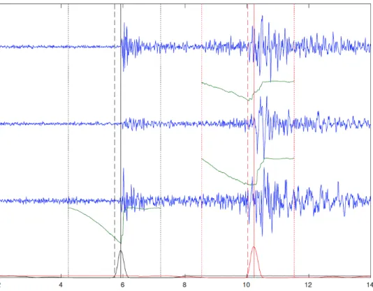
In our workflow, we also implemented an optional AIC phase-picker (Maeda, 1985; Zhang et al., 2003) for applications that do not have sufficient number of robust manual phase picks to train the attention U-Net. The AIC is computed for a 3-second time window centered on the P- or S-wave arrival time predicted using the origin time and hypocenter location estimated in the back-projection process (Figure 8). The P-wave arrival time is picked on the vertical-component seismogram, while the S-wave arrival time is picked on the horizontal-component seismogram with higher SNR. In this study, we applied both the attention U-Net and the AIC phase picker to obtain arrival times. The results obtained using both methods were generally consistent with each other. When the difference was less than 0.1 s, we used the pick of the attention U-Net. When the
difference was larger than 0.1 s, we used the one with higher SNR.
3.3.2. Re-location
The P- and S-wave arrival times were then used to invert for a new origin time and hypocenter location for the template source using Simul2000 (Thurber & Eberhart-Phillips, 1999) and the 3D seismic velocity model CVM-S4.26. For each source inversion, we required at least 4 stations and 8 arrival times and we assigned higher weights to the arrival times with higher SNR. After the source inversion, we rejected the earthquakes located outside of our study volume and also those with horizontal location error larger than 2.5 km or vertical location error larger than 5 km. The total number of accepted template sources used for small earthquake detection in the following template-matching process was over 32,000.
3.3.3. Magnitude estimation
The exact formulation for estimating the local magnitudes may depend upon regional geological conditions and is often network-specific. In Southern California, the local magnitude, ML, is determined using a revised formulation with station corrections
(Hutton et al., 2010). Currently, the constants for the station corrections can be obtained only through personal communication (Hutton et al., 2010). In this study, the magnitudes
of our template events were estimated based upon a three-step approach. For each template source, we first identified the 3 closest earthquakes in the SCSN catalog, and then we calculated the maximum amplitude ratios between the waveforms of the SCSN events and those of the template source, and in the last step we took the median of the ratios and used the 10-based logarithm relationship between the amplitude and one magnitude unit to estimate the magnitude of the template source.
3.4. Template matching for small earthquake detection
The template waveforms used in our TMA process were obtained by windowing the seismograms of the template sources surrounding the P- and/or S-wave. For waveform processing, we remove linear trend, and then apply a taper to the waveforms before filtering. A fourth-order 2-10 Hz Butterworth bandpass filter is applied to the recordings. To reduce the computational resources, we decimate the processed waveforms to 50 samples per second. In this study, we used a 3-second-long time window starting 0.2 s before the arrival time of the P- or S-wave. We found that this time window is long enough to capture the characteristic shapes of the waveforms used in our study, while not too long to increase the computational cost substantially.
Our TMA process generally followed those in previous studies (e.g., Shelly et al., 2007; Peng & Zhao, 2009; Mu et al., 2017). We used the 12 times median absolute deviation (MAD) of the daily sum of NCC series as the threshold for new event detection. We note that our threshold is actually higher than the value commonly used in previous studies, which is ~9 times of the MAD (e.g., Peng & Zhao, 2009). If the origin times of multiple newly detected events are within 2 seconds, the event with the highest MAD was selected as the new event and the other events were rejected. The hypocenter location of a
template source was assigned to all the events detected using its template waveforms. The GPU-accelerated TMA code “cuNCC” developed in Mu et al. (2017) was used in this study and it took less than 3 hours of wall-time on a desktop computer equipped with 8 Nvidia GeForce RTX 1080 Ti GPU cards to match one daylong 3-component
continuous recordings at all the stations with all template waveforms from over 32,000 template sources.
4. Results
At the time of writing, we have completed processing the 3-component continuous recordings at the 22 stations from 1 July 2019 to 30 September 2019 using GAMMA. More recordings are still being processed and new results and findings will be
documented in future publications. The main contribution of this study is a catalog of foreshocks and aftershocks associated with the Ridgecrest earthquake sequence. At the current stage, the number of earthquakes detected using GAMMA has exceeded ~700,000, which is more than 21 times the total number of earthquakes reported in the SCSN catalog.
Figure 1c shows the lateral and depth distributions of the hypocenters in the Ridgecrest sequence we have detected so far. The lateral distribution of the hypocenters in our catalog is generally consistent with that in the SCSN catalog (Figure 1b), while there are visible differences in the details, especially around the intersection between the NW-SE trending LLFZ and the previously unspecified NE-SW trending fault zone. The
differences in the depth distributions of the hypocenters between our catalog and the SCSN catalog are more obvious. We speculate that a substantial portion of the hypocenter differences between our catalog and the SCSN catalog comes from the differences in the seismic velocity models used for locating the earthquakes.
Figure 9a shows a comparison of the temporal variations of the number of earthquakes per day in the Ridgecrest sequence in our catalog and in the SCSN catalog. The
magnitudes of completeness are about 1.0 and -0.6 for the SCSN and the GAMMA catalogs, respectively. As expected, the number of detected earthquakes per day decreases with time. However, the rate of the decrease appears to be slow. This observation is probably related to the complex faulting processes of the Ridgecrest sequence and the triggered earthquakes in Coso geothermal region. Declustering methods are probably needed for a more detailed aftershock behavior analysis (e.g. Ouillon and Sornette, 2005). Another subtle difference between our catalog and the SCSN catalog is the time of peak seismicity. The SCSN catalog shows a clear peak immediately after the Mw 7.1 mainshock, while our catalog shows a less obvious peak in seismicity about 2
days after the mainshock. The exact cause of this difference in the time of peak seismicity is still under investigation.
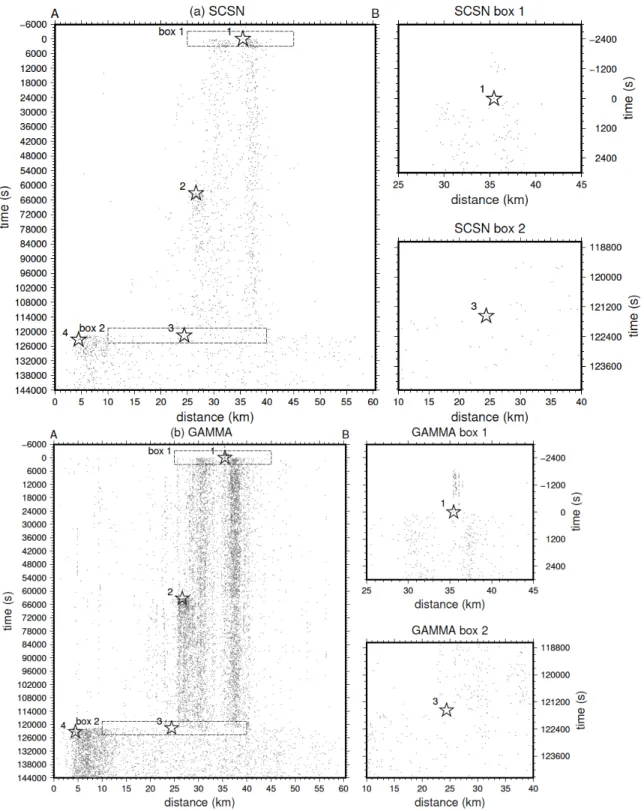
Figure 10 shows a comparison of the temporal variations of seismicity along the strike of the NW-SE trending LLFZ between our catalog and the SCSN catalog. Both catalogs show foreshock activities before the Mw 6.4 earthquake (figure 10). In GAMMA catalog, there are more foreshocks being identified and some of them are about 10 minutes before the mainshock and are missed in the SCSN catalog (figure 10b). Immediately following the Mw 6.4 foreshock, seismicity mainly concentrated within two narrow bands on both
sides of the foreshock epicenter. The northern seismicity band extended slightly further north after the Mw 5.4 earthquake. This general pattern terminated at the Mw 7.1
mainshock, whose epicenter was slightly north of the Mw 5.4 event earlier. After the
mainshock, the two predominant seismicity bands surrounding the Mw 6.4 foreshock
disappeared and the main seismicity shifted abruptly to the north by ~20 km. This northern-most seismicity band appeared to be bounded by the epicenter of the Mw 5.5
aftershock occurred ~30 minutes after the mainshock.
5. Summary and Discussions
In this study, we have developed a systematic, automatic and scalable solution, code named “GAMMA”, to address the major challenges associated with applying TMA-based techniques for routine (near) real-time detection and location of seismic events. To address the challenge associated with the high computational cost of TMA, we developed the GPU-accelerated TMA code “cuNCC”, which reduces the computing time by nearly 3 orders of magnitude. To provide a systematic and automatic approach for establishing
the template waveform database, we developed a GPU-accelerated back-projection code for identifying template sources and an automatic phase-picking algorithm based on the attention U-Net to invert arrival time picks for improved origin times and hypocenter locations of the template sources. The successful application of GAMMA to the
Ridgecrest foreshock-mainshock-aftershock sequence demonstrated the effectiveness and efficiency of our approach.
At the current stage, the small events detected using TMA (section 3.4) were assigned the same hypocenter locations as their corresponding template sources. The cross-correlation processes during TMA also provide the differential travel-time measurements between the template source and the newly detected small event. Such differential travel-time data can be used to invert for highly accurate, relative location between a small event and its corresponding template source. Open-source codes, such as hypoDD (Waldhauser, 2001), GrowClust (Trugman & Shearer, 2017), XCORLOC (Lin, 2018), can be adopted to relocate the small events using the differential travel-time measurements.
The completeness of the small event catalog determined using GAMMA depends upon two interrelated factors: the density of the seismic network and the completeness of the template waveform database. Because our template source selection criterion prefers sources with higher SNR, the selected template sources tend to have relatively larger magnitudes and are less affected by seismic network density. However, because our assumption is that as long as the hypocenter locations and source mechanisms are similar, the waveforms from smaller events should have similar shapes as those from larger events at the same station locations, the completeness of our template waveform database will be adversely affected if smaller events are systematically and substantially different from larger events in hypocenter locations and/or source mechanisms.
The completeness of the catalog obtained using GAMMA is affected by seismic network density, which is inevitable for any practical detection techniques. In this study, we selected 22 stations surrounding the Ridgecrest sequence (Figure 1), because including more stations did not change significantly the total number of detected events. The waveform SNR at more distant stations was too low to be used for reliable TMA-based detection of small events (ML < 1) in the Ridgecrest sequence. Our experiment using the
Ridgecrest sequence suggests a straightforward approach for scaling GAMMA to large seismic networks covering vast areas. For the purpose of small event detection, we can simply divide a large seismic network into multiple overlapping “virtual networks” with each covering a localized area. The boundary of a virtual network can be determined by the SNR of the smallest target event in the localized area. In such a setup, GAMMA can be applied independently to all virtual networks in parallel with negligible
intercommunication overheads. With such a parallelization scheme, we expect GAMMA to become a useful alternative to conventional triggering-based, (near) real-time detection and location routines used by seismic networks around the world.
at http://bit.ly/2WswZQk (last accessed October 2019). The Southern California Seismic Network (SCSN) earthquake catalog website is
http://service.scedc.caltech.edu/eq-catalogs/date_mag_loc.php (last accessed October 2019). The seismic waveforms used in this study were obtained from the Southern California Earthquake Data Center (SCEDC) through the Seismogram Transfer Program (STP) and the website of STP is
https://scedc.caltech.edu/research-tools/stp-index.html (last accessed October 2019). The SCSN station information website is at https://scedc.caltech.edu/station/ (last accessed October 2019).
Reference:
Chen, P., & Lee, E. J. (2015). Full-3D Seismic Waveform Inversion: Theory, Software
and Practice. Springer.
Çiçek, Ö., Abdulkadir, A., Lienkamp, S.S., Brox, T., Ronneberger, O., 2016. 3D U-Net: Learning Dense Volumetric Segmentation from Sparse Annotation, in: Ourselin, S., Joskowicz, L., Sabuncu, M.R., Unal, G., Wells, W. (Eds.), Medical Image Computing and Computer-Assisted Intervention – MICCAI 2016, Lecture Notes in Computer Science. Springer International Publishing, pp. 424–432.
Croft, J. and Goyette, B., July 4, 2019. California earthquake felt in Los Angeles and Las Vegas. CNN. Retrieved July 4, 2019.
Gibbons, S.J., Ringdal, F., 2006. The detection of low magnitude seismic events using array-based waveform correlation. Geophys. J. Int. 165, 149–166. doi:10.1111/j.1365-246X.2006.02865.x
Hutton, K., Woessner, J., Hauksson, E., 2010. Earthquake Monitoring in Southern California for Seventy-Seven Years (1932-2008). Bulletin of the Seismological Society of America 100, 423–446. https://doi.org/10.1785/0120090130
Kao, H., Kan, C.-W., Chen, R.-Y., Chang, C.-H., Rosenberger, A., Shin, T.-C., Leu, P.-L., Kuo, K.-W., Liang, W.-T., 2012. Locating, monitoring, and characterizing typhoon-linduced landslides with real-time seismic signals. Landslides 9, 557–563.
https://doi.org/10.1007/s10346-012-0322-z
Langet, N., Maggi, A., Michelini, A., Brenguier, F., 2014. Continuous Kurtosis-Based Migration for Seismic Event Detection and Location, with Application to Piton de la Fournaise Volcano, La Reunion. Bulletin of the Seismological Society of America 104, 229–246. https://doi.org/10.1785/0120130107
Lee, E., Chen, P., 2016. Improved Basin Structures in Southern California Obtained Through Full-3D Seismic Waveform Tomography (F3DT). Seismological Research Letters 87, 874–881. https://doi.org/10.1785/0220160013
Lee, E.-J., Chen, P., Jordan, T.H., Maechling, P.B., Denolle, M.A.M., Beroza, G.C., 2014. Full-3-D tomography for crustal structure in Southern California based on the scattering-integral and the adjoint-wavefield methods. J. Geophys. Res. Solid Earth 119, 6421–6451. https://doi.org/10.1002/2014JB011346
Lee, E.-J., Liao, W.-Y., Lin, G.-W., Chen, P., Mu, D., Lin, C.-W., 2019. Towards Automated Real-Time Detection and Location of Large-Scale Landslides through Seismic Waveform Back Projection. Geofluids 2019, 1–14.
https://doi.org/10.1155/2019/1426019
Liao, W.-Y., 2019. Using deep learning for the seismic phase identification and its potential applications. National Cheng Kung University. (in preparation for submission). https://doi.org/10.6844/NCKU201900617
Lin, G. (2018). The source-specific station term and waveform cross-correlation earthquake location package and its applications to California and New
Zealand. Seismological Research Letters, 89(5), 1877-1885.
Maeda, N., 1985. A Method for Reading and Checking Phase Time in Auto-Processing System of Seismic Wave Data. Zisin (Journal of the Seismological Society of Japan. 2nd ser.) 38, 365–379. https://doi.org/10.4294/zisin1948.38.3_365
Mu, D., Lee, E.-J., Chen, P., 2017. Rapid earthquake detection through GPU-Based template matching. Computers & Geosciences 109, 305–314.
https://doi.org/10.1016/j.cageo.2017.09.009
Oktay, O., Schlemper, J., Folgoc, L.L., Lee, M., Heinrich, M., Misawa, K., Mori, K., McDonagh, S., Hammerla, N.Y., Kainz, B., Glocker, B., Rueckert, D., 2018. Attention U-Net: Learning Where to Look for the Pancreas. arXiv:1804.03999 [cs].
Ouillon, G., Sornette, D., 2005. Magnitude-dependent Omori law: Theory and empirical study: MAGNITUDE-DEPENDENT OMORI LAW. Journal of Geophysical Research: Solid Earth 110. https://doi.org/10.1029/2004JB003311
Peng, Z., Gomberg, J., 2010. An integrated perspective of the continuum between earthquakes and slow-slip phenomena. Nat. Geosci. 3, 599–607. doi:10.1038/ngeo940 Peng, Z., Zhao, P., 2009. Migration of early aftershocks following the 2004 Parkfield earthquake. Nat. Geosci. 2, 877–881. doi:10.1038/ngeo697
Ronneberger, O., Fischer, P., Brox, T., 2015. U-Net: Convolutional Networks for Biomedical Image Segmentation. arXiv:1505.04597 [cs].
Ross, Z.E., Meier, M.-A., Hauksson, E., 2018a. P Wave Arrival Picking and First-Motion Polarity Determination With Deep Learning. Journal of Geophysical Research: Solid
Ross, Z.E., Meier, M.-A., Hauksson, E., Heaton, T.H., 2018b. Generalized Seismic Phase Detection with Deep Learning. Bulletin of the Seismological Society of America 108, 2894–2901. https://doi.org/10.1785/0120180080
Ross, Z.E., Trugman, D.T., Hauksson, E., Shearer, P.M., 2019. Searching for hidden earthquakes in Southern California. Science eaaw6888.
https://doi.org/10.1126/science.aaw6888
SCEDC (2013): Southern California Earthquake Data Center. Caltech. Dataset. doi:10.7909/C3WD3xH
Shelly, D.R., Beroza, G.C., Ide, S., 2007. Non-volcanic tremor and low-frequency earthquake swarms. Nature 446, 305–307. doi:10.1038/nature05666
Tan, F., Kao, H., Nissen, E., Eaton, D., 2019. Seismicity-Scanning Based on Navigated Automatic Phase-Picking. Journal of Geophysical Research: Solid Earth 124, 3802–3818. https://doi.org/10.1029/2018JB017050
Thurber, C., Eberhart-Phillips, D., 1999. Local earthquake tomography with flexible gridding. Computers & Geosciences 25, 809–818. https://doi.org/10.1016/S0098-3004(99)00007-2
Trugman, D. T., & Shearer, P. M. (2017). GrowClust: A hierarchical clustering algorithm for relative earthquake relocation, with application to the Spanish Springs and Sheldon, Nevada, earthquake sequences. Seismological Research Letters, 88(2A), 379-391. van der Baan, M., & Calixto, F. J. (2017). Human-induced seismicity and large-scale hydrocarbon production in the USA and C anada. Geochemistry, Geophysics,
Geosystems, 18(7), 2467-2485.
Waldhauser, F. (2001). hypoDD--A program to compute double-difference hypocenter locations.
Wech, A.G., Creager, K.C., 2008. Automated detection and location of Cascadia tremor. Geophysical Research Letters 35. https://doi.org/10.1029/2008GL035458
Wigglesworth, A., July 9, 2019. Expect 34,000 aftershocks from Ridgecrest earthquakes. But seismic activity is slowing down. Los Angeles Times. Retrieved July 10, 2019. Zhang, Z., Liu, Q., Wang, Y., 2018. Road Extraction by Deep Residual U-Net. IEEE Geoscience and Remote Sensing Letters 15, 749–753.
Zhang, H., Thurber, C., Rowe, C., 2003. Automatic P-wave arrival detection and picking with multiscale wavelet analysis for single-component recordings. Bulletin of the
Seismological Society of America 93, 1904–1912.
Zhou, Z., Siddiquee, M.M.R., Tajbakhsh, N., Liang, J., 2018. UNet++: A Nested U-Net Architecture for Medical Image Segmentation. arXiv:1807.10165 [cs, eess, stat].
Zhu, L., Peng, Z., McClellan, J., Li, C., Yao, D., Li, Z., Fang, L., 2019. Deep learning for seismic phase detection and picking in the aftershock zone of 2008 Mw7.9 Wenchuan earthquake. Physics of the Earth and Planetary Interiors 293, 106261.
https://doi.org/10.1016/j.pepi.2019.05.004
Zhu, W., Beroza, G.C., 2018. PhaseNet: A Deep-Neural-Network-Based Seismic Arrival Time Picking Method. Geophysical Journal International.
Caption List
Figure 1. Our study area surrounding the Ridgecrest earthquake sequence. White
triangles: locations of seismic stations; colored dots: epicenters of detected earthquakes in the SCSN catalog before the Ridgecrest sequence (a), after the Ridgecrest sequence (b) and our catalog generated by GAMMA (c); white stars: epicenters of major quakes in the sequence (numbering see Figure 10); black dash line: along strike direction for the horizontal axis in Figure 10. Background gray-scale: regional elevation; color-scale for epicenters: depths of the detected earthquakes.
Figure 2. Schematic diagram of the workflow implemented in GAMMA.
Figure 3. Examples of 3-component seismograms (black solid lines), their kurtosis
functions (blue solid lines), the positive time derivatives of kurtosis functions (red solid lines), and waveform envelopes (magenta solid lines). The vertical solid (man picked) and dash (model predicted) lines indicated the P and S arrivals.
Figure 4. Examples of hourly back-projected and stacked positive time derivatives of the
kurtosis functions (black solid lines) at the grid point closest to the mainshock
hypocenter. Blue vertical lines: origin times of earthquakes in SCSN catalog; red vertical line: origin time of the mainshock; blue stars: origin times of potential template sources; black dash line: the selection threshold used in this study.
Figure 5. Architecture of our attention U-Net for automatic phase picking. Input data
consist of 3-component seismograms; output data are the probabilities of the onset for P-, S- and other wave.
Figure 6. Examples of training data (seismograms in black solid lines) and the “target
functions”, i.e., labels (colored lines in bottom panel) used to train our attention U-Net. Dot-dash lines: manual phase picks provided by SCSN for P- (blue) and S-wave (red).
Figure 7. Comparison of probability predictions made using our attention U-Net (middle)
and the standard U-Net (bottom) for examples of 3-component seismograms (top).
Figure 8. Examples of AIC values (green solid lines) and the phase picks for P- (black
solid line) and S-waves (red solid line) on a 3-component seismogram. Black and red solid lines on the bottom show probability functions predicted using our attention U-Net. Dash lines are the predicted P (black) and S (red) arrivals based on back-projection results. Dotted lines indicate the ±1.5s time windows of predicted arrivals for P (black) and S (red) phase selections.
Figure 9. (a) Number of earthquakes per day detected using GAMMA (blue bars) and
provided in the SCSN catalog (orange bars) as a function of Julian day. Red stars: origin times of the earthquakes with Mw > 5. Magnitude and cumulative number of earthquakes
Figure 10. Temporal variations (vertical axis) of seismicity along the strike of the
NW-SE trending LLFZ (horizontal axis, see Figure 1bc) for events in the SCSN catalog (a) and our catalog generated using GAMMA (b). The earthquakes within ± 4 km along the A-B dash line in Figure 1bc are selected. Stars from top to bottom, right to left: the epicenters of the Mw 6.4 foreshock, the Mw 5.4 event, the mainshock and the Mw 5.5
aftershock. The time of earthquakes are relative to the origin time of the Mw 6.4 Earthquake in the 2019 Ridgecrest earthquake sequence.
Figures
Figure 1. Our study area surrounding the Ridgecrest earthquake sequence. White
triangles: locations of seismic stations; colored dots: epicenters of detected earthquakes in the SCSN catalog before the Ridgecrest sequence (a), after the Ridgecrest sequence (b) and our catalog generated by GAMMA (c); white stars: epicenters of major quakes in the sequence (numbering see Figure 10); black dash line: along strike direction for the horizontal axis in Figure 10. Background gray-scale: regional elevation; color-scale for epicenters: depths of the detected earthquakes.
Figure 3. Examples of 3-component seismograms (black solid lines), their kurtosis functions (blue solid lines), the positive time derivatives of kurtosis functions (red solid lines), and waveform envelopes (magenta solid lines). The vertical solid (man picked) and dash (model predicted) lines indicated the P and S arrivals.
Figure 4. Examples of hourly back-projected and stacked positive time derivatives of the kurtosis functions (black solid lines) at the grid point closest to the mainshock
hypocenter. Blue vertical lines: origin times of earthquakes in SCSN catalog; red vertical line: origin time of the mainshock; blue stars: origin times of potential template sources; black dash line: the selection threshold used in this study.
Figure 5. Architecture of our attention U-Net for automatic phase picking. Input data consist of 3-component seismograms; output data are the probabilities of the onset for P-, S- and other wave.
Figure 6. Examples of training data (seismograms in black solid lines) and the “target functions”, i.e., labels (colored lines in bottom panel) used to train our attention U-Net. Dot-dash lines: manual phase picks provided by SCSN for P- (blue) and S-wave (red).
Figure 7. Comparison of probability predictions made using our attention U-Net (middle) and the standard U-Net (bottom) for examples of 3-component seismograms (top).
Figure 8. Examples of AIC values (green solid lines) and the phase picks for P- (black solid line) and S-waves (red solid line) on a 3-component seismogram. Black and red solid lines on the bottom show probability functions predicted using our attention U-Net. Dash lines are the predicted P (black) and S (red) arrivals based on back-projection results. Dotted lines indicate the ±1.5s time windows of predicted arrivals for P (black) and S (red) phase selections.
Figure 9. (a) Number of earthquakes per day detected using GAMMA (blue bars) and provided in the SCSN catalog (orange bars) as a function of Julian day. Red stars: origin times of the earthquakes with Mw > 5. Magnitude and cumulative number of earthquakes
Figure 10. Temporal variations (vertical axis) of seismicity along the strike of the NW-SE trending LLFZ (horizontal axis, see Figure 1bc) for events in the SCSN catalog (a) and our catalog generated using GAMMA (b). The earthquakes within ± 4 km along the A-B dash line in Figure 1bc are selected. Stars from top to bottom, right to left: the epicenters of the Mw 6.4 foreshock, the Mw 5.4 event, the mainshock and the Mw 5.5 aftershock. The
106年度專題研究計畫成果彙整表
計畫主持人:李恩瑞 計畫編號:106-2628-M-006-001-MY3 計畫名稱:一個基於圖形處理器(GPU)的即時微震監測平台 成果項目 量化 單位 質化 (說明:各成果項目請附佐證資料或細 項說明,如期刊名稱、年份、卷期、起 訖頁數、證號...等) 國 內 學術性論文 期刊論文 0 篇 研討會論文 0 專書 0 本 專書論文 0 章 技術報告 0 篇 其他 0 篇 國 外 學術性論文 期刊論文 7 篇 計畫第一年1. Mu, D., Lee, E. J., & Chen, P. (2017, Dec). Rapid earthquake detection through GPU-Based template matching. Computers and Geosciences, 109, 305-314.
https://doi.org/10.1016/j.cageo.201 7.09.009
計畫第二年
1. Wang, W., Chen, P., Keifer, I., Dueker, K., Lee, E. J., Mu, D., Jiao, J., Zhang, Y., & Carr, B. (2019, Mar). Weathering front under a granite ridge revealed through full-3D seismic ambient-noise tomography. Earth and Planetary Science Letters, 509, 66-77.
https://doi.org/10.1016/j.epsl.2018 .12.038
2. Lee, E. J., Rau, R. J., Chen, P., Mu, D., & Lin, C. M. (2019, Feb). Coseismic velocity variations associated with the 2018 M w 6.4 Hualien earthquake estimated using repeating earthquakes Seismological Research Letters, 90(1), 118-130. https://doi.org/10.1785/0220180230 3. Lee, E. J., Liao, W. Y., Lin, G. W., Chen, P., Mu, D., & Lin, C. W. (2019, Jan). Towards automated real-time detection and location of
seismic waveform back projection. Geofluids, 2019, [1426019].
https://doi.org/10.1155/2019/142601 9
計畫第三年
1. Wang, W., Chen, P., Dueker, K., Lee, E. J., Mu, D., & Keifer, I. (2020, Nov). Seismic evidence of glacial deposits inhibiting weathering of local bedrock at a snow-dominated subalpine watershed. Earth and Planetary Science
Letters, 549, [116517].
https://doi.org/10.1016/j.epsl.2020 .116517
2. Lee, E. J., Mu, D., Wang, W., & Chen, P. (2020, Aug). Weighted template-matching algorithm (WTMA) for improved foreshock detection of the 2019 ridgecrest earthquake sequence. Bulletin of the
Seismological Society of America, 110(4), 1832-1844.
https://doi.org/10.1785/0120200020 3. Lee, E. J., Liao, W. Y., Mu, D., Wang, W., & Chen, P. (2020, Jul). GPU-accelerated automatic
microseismic monitoring algorithm (GAMMA) and its application to the 2019 ridgecrest earthquake
sequence. Seismological Research Letters, 91(4), 2062-2074.
https://doi.org/10.1785/0220190323
研討會論文 1
計畫第一年
Mu, D., Lee, E. J., Cicotti, P., Langer, F. J., Cui, Y., Qiu, J., Lee, H. J., & Morrin, C. (2018, Jul). Deep learning for seismic template recognition. Practice and Experience in Advanced Research Computing 2018: Seamless
Creativity, PEARC 2018 [a58] (ACM International Conference Proceeding Series). Association for Computing Machinery.
專書論文 0 章 技術報告 0 篇 其他 0 篇 參 與 計 畫 人 力 本國籍 大專生 3 人次 計畫第一年 何立新 計畫第二年 黃籍億 計畫第三年 張家瑋 碩士生 8 計畫第一年 何宗璟、蕭欣宜、廖勿渝、許沛然 計畫第二年 何宗璟、蕭欣宜、廖勿渝、許沛然、黃 籍億、康倫愷 計畫第三年 廖勿渝、黃籍億、葉儒、林容辰 博士生 0 博士級研究人員 0 專任人員 1 計畫第一年~計畫第三年 吳秉芬 非本國籍 大專生 0 碩士生 0 博士生 0 博士級研究人員 0 專任人員 0 其他成果 (無法以量化表達之成果如辦理學術活動 、獲得獎項、重要國際合作、研究成果國 際影響力及其他協助產業技術發展之具體 效益事項等,請以文字敘述填列。)