Adaptive variable structure control

(1)

Adaptive variable structure

control

C.-J. Chien and L.-C. Fu

3.1 Introduction

In the past two decades, model reference adaptive control (MRAC) using only input/output measurements has evolved as one of the most soundly developed adaptive control techniques. Not only has the stability property been rigor- ously established [17], [19] but also the robustness issue due to unmodelled dynamics and input/output disturbance has been successfully solved [15], [18]. However, several limitations on MRAC remain to be relaxed, especially the problem of unpredictable transient response and tracking performance which has recently become one of the challenging research topics in the field of MRAC. A considerable amount of effort has been made to improve these schemes to obtain better control effects [6], [9], [11], [22]. One effort out of several is to try to incorporate the variable structure design (VSD) [9], [11] concept into the traditional model reference adaptive controller structure. Notably, Hsu and Costa [11] have first successfully proposed a plausible scheme in this line, which was then followed by a series of more general results [12], [13], [14]. Aside from those, Fu [9], [10] has taken up a different approach in placing the variable structure design in the overall resulting adaptive controller. An offspring of the work [9] and part of the work [12] include various versions of results respectively applied to SISO [20], [23], MIMO [2], [5], time-varying [4], decentralized [24] and affine nonlinear [3] systems.

It is well known that a main difficulty for the design of the variable structure MRAC system is the so-called general case when relative degree of the plant is greater than one. In this chapter, we present a new algorithm to solve the variable structure model reference adaptive control for a single input single output system with unmodelled dynamics and output disturbances. The design concept will be first introduced for relative degree-one plants and then be

(2)

42 Adaptive variable structure control

extended to the general ease. Compared with the previous works, which used adaptive variable structure design or traditional robust adaptive approaches for the MRAC problem, this algorithm has the following special features: (1) This control algorithm successfully applies the variable structure adaptive

controller for the general ease under robustness consideration.

(2) The control strategy using the concept of 'average control' rather than that of 'equivalent contror is thoroughly analysed.

(3) A systematic design approach is proposed and a new adaptation mechan- ism is developed so that the prior upper bounds on some appropriately defined but unavailable system parameters are not needed. It is shown that without any persistent excitation the global stability and robustness with asymptotic tracking performance can be guaranteed. The output tracking error can be driven to zero for relative degree-one plants and to a small residual set (whose size depends on the level of magnitude of some design parameter) for plants with any higher relative degree. Both results are achieved even when the unmodelled dynamic and output disturbance are present.

(4) If the aforementioned bounds on the system parameters are available by some means before controller design, then with a suitable choice of initial control parameters, the output tracking error can even be driven to zero in finite time for relative degree-one plants and to a small residual set exponentially for plants with any higher relative degree. It is noted that these bounds are usually assumed to be known before the construction of the variable structure controller or the robust adaptation law.

In order to make a comparison between the proposed adaptive variable structure scheme and the traditional approaches, some computer simulations are made to illustrate the differences of the tracking performance. The simulations will clearly demonstrate the excellent transient responses as well as tracking performance, which are almost never possible to achieve when traditional MRAC schemes are employed [19].

The theoretical framework in this chapter is developed based on Filippov's solution concept for a differential equation with discontinuous fight-hand side [8]. In the subsequent discussions, the following notations will be used: (1)

P(s)[u](t):

denotes the filtered version of

u(t)

with any proper or strictly

proper transfer function

P(s).

(2) I" l: denotes the absolute value of any scalar or the Euclidean norm of any vector or matrix.

(3)

II('),lio~

= supr__.t

I(')(r)l:

denotes the truncated Loo norm of the argument function or vector.

(4) Ile(s)lloo

" denotes the Hoo norm of the transfer function

P(s).

(3)

description, control objective and then derive the MRAC based error model. In Section 3.3, the adaptive variable structure controller for relative degree-one plants is proposed with stability and performance analysis. The extension to plants with relative degree greater than one is presented in Section 3.4. Section 3.5 gives simulation results to demonstrate the effectiveness of the adaptive variable structure controller. Finally, a conclusion is made in Section 3.6.

3.2 Problem formulation

3.2.1 Plant description and control objective

In this chapter, we consider the following SISO linear time-invariant plant described by the equation:

yp(t)

= P(s)(1 +

#Pu(s))[up](t) + do(t)

(3.1) where

up(t)

and

yp(t)

are plant input and plant output respectively,

#Pu(s)

is the multiplicative unmodelled dynamics with some # E R +, and

do

is the output disturbance. Here,

P(s)

represents the strictly proper rational transfer function of the nominal plant which is described by

rip(s)

(3.2)

P(s) =

kp dp(s)

where

np(s)

and

dp(s)

are some monic coprime polynomials and kp is the high frequency gain. Now suppose that the plant (3.1) is not precisely known but some prior knowledge about the transfer function may be available. The control objective is to design an adaptive variable structure control scheme such that the output

yp(t)

of the plant will track the output

ym(t)

of a linear time-invariant reference model described by

~m(~)

ym(t) = M(s)[rm](t) =km dm(si [rm](t)

(3.3)

where

M(s)

is a stable transfer function and

rm(t)

is a uniformly bounded reference input. In order to achieve such an objective, we need some assumptions on the modelled part of the plant and the reference model as well as the unmodelled part of the plant. These assumptions are made in the following.

For the modelled part of the plant and reference model:

(A1) All the coefficients of

np(s)

and

dp(s)

are unknown a priori, but the order of

P(s)

and its relative degree are known to be n and p, respectively. Without loss of generality, we will assume that the order of

M(s)

and its relative degree are also n and

p,

respectively.

(4)

(A2) The value of high frequency gain

k v

is unknown, but its sign should be known. Without loss of generality, we will assume

k v,

and hence kin, are positive.

(A3)

P(s)

is minimum phase, i.e. all its zeros lie in the open left half complex plane.

For the unmodelled part of the plant:

(A4) The unmodelled dynamics

Pu(s-kl)

is a strictly proper and stable transfer matrix such that IOl < al, II(eu(s - k t ) s -

D)(s +

a2)[Ioo < al, for some constants al, a2 > 0, where D = lim,__,oo

Pu(s)s

and

IIX(s)lloo - sup. R IXfjw)l [lS].

(A5) The output disturbance is differentiable and the upper bounds on

Ido(t)l, l-~do(t )

exist.

Remark 3.1

9 Minimum-phase assumption (A3) on the nominal plant

P(s)

is to guarantee the internal stability since the model reference control involves the cancella- tion of the plant zeros. However, as commented by [15], this assumption does not imply that the overall plant (3.1) possesses the minimum-phase property.

9 The latter part of assumption (A4) is simply to emphasize the fact that

Pu(s)

are uncorrelated with # in any case [16]. The reasons for assumption (A5) will be clear in the proof of Theorem 3.1 and that of Theorem 4.1.

3.2.2 MRAC based error model

Since the plant parameters are assumed to be unknown, a basic strategy from the traditional M R A C [17], [19] is now used to construct the error model between

yv(t)

and

ym(t).

Instead of applying the traditional MRAC technique, a new adaptive variable structure control will be given here in order to pursue better robustness and tracking performance. Let (3.1) be rewritten as

yp(t) - do(t) = V(s) [up +/zPu(s)[up]]

(t) P(s)[up +

fi](t) (3.4) then from the traditional model reference control strategy [19], it can be shown that there exists O* = [0~,..., 0~n] r E R z~ such that if

, a ( s ) = [o;, o,,..., o*_,1

a(s)

OTe(s )

= [O*, e~,+l,..., O~,_=] ~ - ~ + O~,_,

(5)

polynomial, we have

1 - D*b(S ) -- D~(s)P(s) = ~2,,M -l (s)P(s)

Applying both sides of (3.5) on u~ + ~, we have

up(t)+~(t)-D;(s)[up + ~](t)-D~(s)[yp-dol(t)=O~nM-'(s)[yp-do](t )

so that

M(~)O~.-' [u~ +, -

D;(~)t.v + ,] - D;(~)ty~ - do]]

(t)

yp(t) do(t)

Since

D;(s)[up + ill(t) + D~(s)[yp - dol(t) + O~nrm(t )

(3.5)

(3.6) (3.7) - _ o * T D

a(3)

[up + ~](t) " ~(s) [Yp - ao](t)

yp(t) -ao(O

. rm(t) . --- 0 *T

-.(~)

~(s) [UP](t) a(s) yp(t) . rm(t) . 0 a(s) _ o , T ~(S) [d~ do(t) 0 A O,Tw(t) _ O,TWdo (t) + D*b(s)[ff](t )

+ D; (~)[a] (t)

(3.8) we have

yp(t) - do(t) = M(s)O~n-l[up - O'Tw + O*TWdo Jr (1 -- D;(S))[~] q- O~nrm](t )

9 T ,

-- g(s)O*2~l[up - o*Tw "t- 19 Wdo d-/~A(s)[upl h- 02nrm](t ) (3.9)

where A(s) = (1 - D*b(s))Pu(s ) = (1 0~ + ... +O~,_lsn-2~pu(s)" If we define

- 2

x ,

the tracking error eo(t) as y r ( t ) - y m ( t ) , then the error model due to the u n k n o w n parameters, unmodelled dynamics and o u t p u t disturbances can be

(6)

46 Adaptive variable structure c o n t r o l

readily found from (3.3) and (3.9) as follows:

eo(t) = M(s)O~n -1 [up - O*rw + O*TWao 4- #A(s)tue] ]

(t)

+ do(t) (3.10) In the following sections, the new adaptive variable structure scheme is proposed for plants with arbitrary relative degree. However, the control structure is much simpler for relative degree-one plant, and hence in Section 3.3 we will first give a discussion for this class of plants. Based on the analysis for relative degree-one plants, the general case can then be presented in a more straightforward manner in Section 3.4.

3.3 The case of relative degree one

When P(s) is relative degree one, the reference model M(s) can be chosen to be strictly positive real (SPR) (Narendra and Annaswamy, 1988). The error model (3.10) can now be rewritten as

eo(t) = M(s)O[n

I

[u

e -

O*Tw +

o-rwdo*

+ O~nM-' (s)[do]

+

#A(s)[u,]] (t)

(3.11)

In the error model (3.11), the terms

Orw, O-rWao

+O~nM-l(s)[do]

and

#A(s)[up]

are the uncertainties due to the unknown plant parameters, output

disturbance, and unmodelled dynamics, respectively. Let

(Am,

Bin,

Cm) be

any

minimal realization of

M(s)O~,

-l

which is SPR, then we can get the following

state space representation of (3.1 I) as:

~(t)

=

Ame(t)+Bm(u~(t)--Orw(t)+O-rWdo

(t)+O~n

M-l (s)[do](t)+#A(s)[up](t))

eo(t) = Cme(t) (3.12)

where the triplet (Am, Bm, Cm) satisfies

T

emAm + Amem "- -2Qm; emBm = CTm (3.13) for some Pm= Pm r > 0 and Qm -- Qrm > O.

The adaptive variable structure controller for relative degree-one plants is now summarized as follows:

(1)

Define the regressor signal

w(t) =

ra(s)t~(~) [uel(t),

a(s)

_]

T

~(-~ [yp](t), yp(t), rm(t) = [wl(t),w2(t),...,w2n(t)] T

(7)

and construct the normalization signal m(t) [15] as the state of the following system:

(3.15)

a,(t) = - om(t) + 6, + 1), m(0) >

where 6o, 6n > 0 and 6o + 62 < rain (kl, k2) for some 62 > 0. The parameter k2 > 0 is selected such that the roots of A ( s - k2) lie in the open left half complex plane, which is always achievable.

(2) Design the control signal up (t) as

2n

up(t) = ~ ( - s g n (eowj)Oj(t)wj(t)) - sgn (eo)31(t) - sgn ( e o ) ~ ( t ) m ( t ) (3.16)

j=l

1 if eo > 0 s g n ( e o ) = 0 if e 0 = 0

- 1 if eo < 0

(3) The adaptation law for the control parameters is given as Oj(t)='Tjleo(t)wj(t)l , j = 1 , . . . , 2 n

~l (t) ~--- gl]eo(t)]

~(t)

=

02[eo(t)]m(t)

(3.17)

where ~0,gl,g2 > 0 are the adaptation gains and 07(0), 31 (0),/32(0) > 0 (in general, as large as possible)j - I,..., 2n.

The design concept of the adaptive variable structure controller (3.15) and (3.16) is simply to construct some feedback signals to compensate for the uncertainties because of the following reasons:

9 By assumption (A5), it can be easily found that [O*Twc,(t)+ O~,M(s)-l[ao](t)l < 3~ for some ~ > 0.

9 With the construction of m, it can be shown [15] that #A(s)[ur](t ) < ~ m ( t ) , Vt >_ 0 and for some constant/3~ > 0.

Now, we are ready to state our results concerning the properties of global stability, robust property, and tracking performance of our new adaptive variable structure scheme with relative degree-one system.

Theorem 3.1 (Global Stability, Robustness and Asymptotic Zero Tracking Performance) Consider the system (3.1) satisfying assumptions (AI)-(A5) with relative degree being one. If the control input is designed as in (3.15), (3.16) and the adaptation law is chosen as in (3.17), then there exists #* > 0 such that for E [0,#*] all signals inside the closed loop system are bounded and the tracking error will converge to zero asymptotically.

(8)

48 Adaptive variable structure control Proof: Consider the Lyapunov function

2 1

1 (oj -Iql) = + ~ ~ (~j - ~;)'

Va "-" l eT pme "-l- ~ ~Tj

j = l '=

where I'm satisfies (3.13). Then, the time derivative of Va along the trajectory (3.12) (3.17) will be

, T

Va = - e r Q m e + eo(up - o * r w + 0 Wdo + 8~nM-'(s)[do] + IzA(s)[up]) 2 1

-

j=l

2n

<_ - e "r Qme - ~_~ leowyl(oy -I021) -leol(:~ -/~;) - l e o l ( ~ - / ~ ) m 1=1

2. 1 2 1

<__ -qmlel 2

for some constant qm > 0. This implies that e E L2 fq Loo and Oj,j = 1,..., 2n, ~l, ~ , e0 E Loo and, hence, all signals inside the dosed loop system are bounded owing to Lemma A in the Appendix. On the other hand, it can be concluded that d E Loo by (3.12). Hence, e E L2 N Loo and d E Loo readily imply that e and e0 will at least converge to zero asymptotically by Barbalat's lemma

[191.

Q.E.D.

In Theorem 3.1, suitable integral adaptation laws are given to compensate for the unavailable knowledge of the bounds on 10;[ and ~*. Theoretically, the adaptive variable structure controller will stabilize the closed loop system with guaranteed robustness and asymptotic zero tracking performance no matter what 0j(0)'s and/3j(0)'s are. However, according to the following Theorem 3.2, we will expect that positive and large values of 0j(0),~(0) should result in better transient response and tracking performance, especially when

0j(0) > 1031, ~j(0) > ~.

Theorem 3.2 (Finite-Time Zero Tracking Performance with High Gain Design) Consider the system set-up in Theorem 3.1. If 0i(0)> [0;I,~j(0) _ ~ , then the output tracking error will converge to zero in finite time with all signals inside the closed loop system remaining bounded. Proof Consider the Lyapunov function Vb = 89 where Pm satisfies

(9)

(3.13). The time derivative of Vb along the trajectory (3.12) becomes

2n

Vb = -e-rQme- ~_, leowjlCOj- 10;I)- le01(~l - ~ ; ) - le01(~2-/~)m

j = l

<_ --e T Qme <__ - k 3 Vb

for some k3 > 0 since Oj(t)>

1OTl,~(t)> ~*,vt >_ 0.

This implies that e approaches zero at least exponentially fast. Furthermore, by the fact that

,T

eoeo = eo{CmAme + Cmem(up - o*l-w -}" 0 Wdo -I- O~nM-l(s)[do] + pA(s)[ue])}

2n.

<_ k41eollel - ~_, leowjl(Oj -10;I) -le01(~ - / ~ ) -le0l(~ - ~)m

j = l

< k41eollel-

le01 ~ Iwjl(0j -10;I) + (/~l - ~;) + (~2 - N)m

where k4 = ICmAml, and that

lel

approaches zero at least exponentially fast, there exists a finite time Tl > 0 such that eobo < -ksleol for all t > TI and for some k5 > 0. This implies that the sliding surface eo = 0 is guaranteed to be reached in some finite time T2 > Tl > 0. Q.E.D.

Remark 3.2: Although theoretically only asymptotic zero tracking perform- ante is achieved when the initial control parameters are arbitrarily chosen, it is encouraged to set the adaptation gains "b" and gj in (3.17) as large as possible. This is because the large adaptation gains will provide high adaptation speed and, hence, increase the control parameters to a suitable level of magnitude so as to achieve a satisfactory performance as quickly as possible. These expected results can be observed in the simulation examples.

3.4 The case of arbitrary relative degree

When the relative degree of (3.1) is greater than one, the controller design becomes more complicated than that given in Section 3.3. The main difference between the controller design of a relative degree-one system and a system with relative degree greater than one can be described as follows. When (3.1) is relative degree-one, the reference model can be chosen to be strictly positive real (SPR) [19]. Moreover, the control structure and its subsequent analysis of global stability, robustness and tracking performance are much simpler. On the contrary, when the relative degree of (3.1) is greater than one, the reference model M(s) is no longer SPR so that the controller and the analysis technique in relative degree-one systems cannot be directly applied. In order to use the

(10)

similar techniques given in Section 3.3, the adaptive variable structure controller is now designed systematically as follows:

(1) Choose an operator L l ( s ) = : l ( s ) . . . : p - l ( s ) = (s + a l ) .. . (s +

Otp-l)

such that M ( s ) L ~ ( s ) is SPR and denote Li(s) = : / ( s ) . . . f p - l ( s ) , i = 2, . . . , p - 1, Lp(s) = 1.

(2) Define augmented signal

[

1 ]

ya(t) = M ( s ) L I ( S ) Ul -- LI (s) [up] (t) and auxiliary errors

eal (t) = eo(t) + ya(t)

1 1

ea2(t) -" ~ - ~ [U2](t) -- F(rs)[Ul](t)

1 l

ea3(t) = ~ - ~ [u3l(t) -- F - - ~ [u2l(t)

(3.18) (3.19)

(3.20)

I I

eap(t) = l'p-I (S)[ue](t) -- F(rs)[Up_l](t) (3.21)

1

where ~ [ui](t) is the average control of ut(t) with F ( r s ) = (rs + 1) 2, r being small enough. In fact, F ( r s ) can be any Hurwitz polynomial in rs

1

with degree at least two and F(0) = 1. In the literature, F ( r s i is referred to as an averaging filter, which is obviously a low-pass filter whose bandwidth can be arbitrarily enlarged as r ~ 0. In other words, if r is smaller and

1

smaller, the filter F ( r s ) is flatter and flatter.

(3) Design the control signals up, ui, and the bounding function m as follows: 2n

Ul(t) = ~ ( - s g n (ealf4)Oj(t)~(t)) - sgn (eal)t31(t) - sgn (eal)152(t)m(t) j=l

u,(t)

= -sgn

(ea,)

(]ei-I

(,$')

[Ui_l](t )

\I r(rs)

up(t) = u (t)

(3.22) + r / ) , i = 2 , . . . , p (3.23) (3.24)

(11)

with r/> 0 and

1 1 1

~(t) = d l ( S ) " ' d : - i (s) [w](t) = L l ( S ) [wl(t) The bounding function m(t) is designed as the state of the system

(3.25)

rh(t) = -~5om(t) + 8t(lup(t)[ + 1), m(0) > ~0

with/f0,Sl > 0 and 80 +82 < min(kl,k2,cq,...,C~p_l) for some 82 > 0. (4) Finally, the adaptation law for the control parameters Oj,j = 1,..., 2n and

/31,/32 are given as follows"

0j(t) = 7j[eol(t)~(t)l, j = l , . . . , 2 n (3.26)

/~1 (t) -- glleal(t)l (3.27)

/~2(t) = g21eal (t)lm(t) (3.28)

with 0j(0) > 0, 3i(0) > 0 and 7j > 0, #j > 0.

In the following discussions, the construction of feedback signals ~(t), re(t) and the controller (3.22) (3.23) will be clear.

In order to analyse the proposed adaptive variable structure controller, we first rewrite the error model (3.10) as follows:

eo(t) = M(s)[up - 0 ~ - l O . - r w + 0 z l .1- * - o Wdo + 0~-I

q- (0"~ 1 -- 1)uel(t ) q- do(t)

0,_1

1

_O~-I o,-r

2. [O,-rWdo+O;.M-~(s)[ao]]

= M(s)LI (s) Ll (s) [up]- ~J+Li (s)

]

+ Ll (s) [#A (s) [up] + (1 -O~)ue] (t) (3.29)

Now, according to the design of the above auxiliary error (3.18) and error model (3.29), we can readily find that eal always satisfies

0~n_lO.T r 0~; l [O.'rWao + O~nM-l(s)[do]] eal (t) = M(s)LI (s) ul - + LI (s)

]

+ Li (s) [/~A (s) [up] + (1 -O~,)up] (t) (3.30) It is noted that the auxiliary error eal is now explicitly expressed as the output term of a linear system with SPR transfer function M(s)Ll (s) driven by some uncertain signals due to unknown parameters, output disturbances, unmodelled dynamics and unknown high frequency gain sign.

(12)

52 Adaptive variable structure control

Remark

4.1 The construction of the adaptive variable structure controller (3.22) is now clear since the following facts hold:

9 Since Li(s) 0~'-1 [ O*vwd~ +

O~M-' (s)[do]]

(t) is uniformly bounded due to (A5), we have

0~=! [O.TWd ~ + O;M_l(s)[do] ]

(t) < ~; (3.31 /

z,(s)

fo~ s9me ~ .

9 With the design of the bounding function

m(t)

(3.25), it can be shown that

0~.~,'

[#A(s)[up] + (1

-O~n)up]

(t)

LI(S)

<_/~m(t)

(3.32)

for some/3~ > O.

The results described in Remark 4.1 show that the similar techniques for the controller design of a relative degree-one system can now be used for auxiliary error eal. But what happens to the other auxiliary errors ea2,..., eop, especially the real output error eo as concerned? In Theorem 4. l, we summarize the main results of the systematically designed adaptive variable structure controller for plants with relative degree greater than one.

Theorem

4.1 (Global Stability, Robustness and Asymptotic Tracking Performance) Consider the nonlinear time-varying system (3.1) with relative degree p > 1 satisfying (A1)-(A5). If the controller is designed as in (3.18)- (3.25) and parameter update laws are chosen as in (3.26)-(3.28), then there exists r * > 0 and # * > 0 such that for all r E (0,r*) and # E (0,#*), the following facts hold:

(i) all signals inside the closed-loop system remain uniformly bounded; (ii) the auxiliary error e~l converges to zero asymptotically;

(iii) the auxiliary errors

eai,

i = 2 , . . . , p, converge to zero at some finite time; (iv) the output tracking error e0 will converge to a residual set asymptotically

whose size is a class K function of the design parameter r.

Proof

The proof consists of three parts.

Part I

Prove the boundedness of

e~i

and 01,..., 0~,/~l, ~2.

(13)

M(s)Lz (s) is SPR, we have the following realization of (3.20)

0~n-I o*T~ 0~.n -I ,T

~

)

+ t,t (,) [uzx(~)[~A + (1 - 0~,)~A

eal = Clei (3.33)

with PIAl -t- A-~PI = - 2 Q l , PIBI = C-~ for some Pl = P~ > 0 and Ql = Q~ > 0. Given a Lyapunov function as follows:

V, = 89 + ~ ~ Oj - + __(~. _ ~)2 (3.34)

j=l

IO~1

_j=l

2o:

it can be shown by using (3.32) and (3.31) that

V, = -e~Q,e, +

eal --(Ul

-- 0~n-lo*Tr -~- Li(s

)0~n-I

[oTwdo Jr- O~M-l(s)[do]]*

o~-'

)

+ L - ~ [/zA(s)[up] + (1 - O~,,)ut, ]

+ y . ] l ~ 1

j=i ~JJ Oj -- Oj -I- "= ~jj ( ~j -- ~; ) ~j

(,o:f)

<_ -e~Qlel - Z le,,~l 0: - -le=ll(/~, - / ~ ) -leo~l(/~2 - N ) m

:=l

10~,1

j .,,.

= -e-~Qlel < -qllell 2

for some ql > 0 if the controller in (3.22) and update laws in (3.26)--(3.28) are given. This implies that ej, 01,..., 02n, /31, /32 E Loo and eal E L2 Iq Loo.

Step 2 From (3.19)--(3.21), we can find that ea2,... ,eap satisfy

el(~)

Ca2 --" --Otlea2 -I- ZI2 F(TS) [ul]

(14)

54 Adaptive variable structure control

Now by the following facts that for i = 2 , . . . , p: d

"dr (1 e2ai) = eaieai

-- eai (--oti- l eai + Ui

J

\

:~-l(,)

)

F(rs) [Ui-l]

= -ce,_,e2a, + ea,{-sgnCea,)kl ([g~''F(7"s)cs) [u,_,] _{+ rl}

Ei-I (S)

_{F(rs) [Ui-I ]}

}

o r

,4

--" leail < - a i - l leail - rl

dt - (3.35)

when leo~l # o. This implies that eai will converge to zero after some finite time T > 0 .

Part H Prove the boundedness of all signals inside the closed loop system. Define e-ai = M(s)Li-l (s)[eai], i = 2, . . . , p and Ea = eal + ea2 + " " + eat, which is uniformly bounded due to the boundedness of eai. Then, from (3.18)--(3.21), we can derive that

[

'

]

Ea = eo + M(s)LI (s) ul - L - ~ [up]

[,

, ]

+ M ( s ) L , (s) el (s)[u2]- F(rs) [u'l

[,

,

]

+ M(s)Lz(s) d2(s)[u3l

- ~

[u2l

I1

,

]

+ M(,)L,_,(,) :,~(s)[u,]-F-(~[u,-,]

(1

l

~)

M(s)L~(~) Ul +

[

1

[u21 + . . . +

,

[uo-~]

l

= eo + F ~ s :i (S) el (s)...

dp_2(s)

~= e0 + R (3.36)

Now, since

II(u~),ll~ ~ k611(e0),ll~ +

k6, i = 1 , . . . , p - 1 for some k6 > 0 by Lemma A in the appendix, it can be easily found that

(15)

for some k7 > 0. Furthermore, since the H ~ norm of

II ~

(1 - F--~)lloo = 2r and

[[sM(s)LI

(s)ll~

= k8 for some ks > 0, we can conclude that

'l(R)"l~176 1 F< s))l

I[ sM(s)LI(s) (kTll(eo)tll~+ k7)

o o o o

_< r(k9ll(eo),lloo + k9)

for some k9 > 0. Now from (3.36) we have

II(eo),ll~o ___

II(Ea),ll~ +

II(R),iI~ --- II(Ea),lloo + r(k91l(eo)tll~ + k9)

which implies that there exists a r* > 0 such that 1 - "r'k9 > 0 and for all

r ~ (0, r*)"

II(Ea),II~ q-

"rk9

II(e0),lloo -<

1

- rk9

(3.37)

Combining Lemma A and (3.37), we readily conclude that all signals inside the closed loop system remain uniformly bounded.

Part IIl: Investigate the tracking performance of eal and e0.

Since all signals inside the closed loop system are uniformly bounded, we have

eal E L2 CI Loo, eal E Loo

Hence, by Barbalat's lemma, e~l approaches zero asymptotically and Ea = eal + ~a2 + " " + e.ap also approaches zero asymptotically. Now, from the fact of (3.37) and E~ approaching zero, it is clear that e0 will converge to a small residual set whose size depends on the design parameter r. Q.E.D. As discussed in Theorem 3.2, if the initial choices of control parameters Oj(O) ~(0) satisfy the high gain conditions Oj(O) > 0~ and ~j(0) > /~;, then, by using the same argument given in the proof of Theorem 3.2, we can guarantee the exponential convergent behaviour and finite-time tracking performance of all the auxiliary errors ea~. Since eai reaches zero in some finite time and Ea = eal + P.a2 + " " + ~ap, it can be concluded that Ea converges to zero exponentially and e0 converges to a small residual set whose size depends on the design parameter r. We now summarize the results in the following Theorem 4.2.

Theorem 4.2: (Exponential Tracking Performance with High Gain Design) Consider the system set-up in Theorem 4.1. If the initial value of control parameters satisfy the high gain conditions 0y(0) > 0~ and/~y(0) > ~ , then

- e ~ ,

there exists a r* and #* such that for all r E (0,r*] and # E (0,#*], the following facts hold:

(16)

(ii) the auxiliary errors eai, i = 1 , . . . , p, converge to zero in finite time; (iii) the output tracking errors e0 will converge to a residual set exponentially

whose size depends on the design parameter r.

Remark 4.2: It is well known that the chattering behaviour will be observed in the input channel due to variable structure control, which causes the implementation problem in practical design. A remedy to the undesirable phenomenon is to introduce the boundary layer concept. Take the case of relative degree one, for example, the practical redesign of the proposed adaptive variable structure controller by using boundary layer design is now stated as follows:

up(t) = ~ -Ir(eowj)Oy(t)wy(t) - lr(eo)/~l (t) - lr(eo)/~2(t)m(t) (3.38) sgn (eo) if le01 > e

It(e0) = e0 if le0] <_e

for some small ~ > 0. Note that ~r(e0) is now a continuous function. However, one can expect that the boundary layer design will result in bounded tracking error, i.e. e0 cannot be guaranteed to converge to zero. This causes the parameter drift in parameter adaptation law. Hence, a leakage term is added into the adaptation law as follows:

Oj(t) = "~j[eo(t)wj(t)[ - tzOj(t), j = 1 , . . . , 2n

/~1 (t) =

gl le0(t)l

-

a/~l (t)

~ ( t ) -- g2leo(t)lm(t) - a/~2(t) (3.39) for some cr > 0.

3.5 Computer simulations

The adaptive variable structure scheme is now applied to the following unstable plant with unmodelled dynamics and output disturbances:

8 (l+O.O1

1 )

yp(t) = s3 + s2 + s - 2 s + 10 [up](t) + 0.05 sin(5t)

Since the nominal plant is relative degree three, we choose the following steps to design the adaptive variable structure controller:

(17)

9 reference model and reference input: M(~) = - - - (s + 2) 3

r m ( t ) = { 2

--2

if t < 5 i f 5 < t < l O 9 design parameters: Ll (s) = el (s)d2(s), el (s) = s + 1, ~2(s) = s + 2 A(s) = (s + 1) 2 F(rs) = ( I s + 1) 2

9 augmented signal and auxiliary errors:

[ l ]

ya(t) = M(s)LI (s) Ul

-- Ll (s) [Up]

(t)

eal (t) "- eo(t) + ya(t)

1 1

ea2(t)

=/'1 (s)[u2](t) -

F('rs)[Ul](t)

1 1

ea3(t)

=/'2(s) [u3](t) -

F(~'S)[u2](t)

9 controller:

u~(t)

= ~ - s g n

(e.~)oj(t)~(t) -sgn (eal)~l(t)

- - s g n

(e.~)~2(t)m(t)

u,(t) = - s g n (e.,)

]F(rs)

[U,_l](t) + 1 , i = 2,3

Up(t) -- Up(t)

rh(t) = -m(t) + O.O05([up(t)] +

1), m(O) -- 0.2 9 adaptation law:

Oj(t) = 7jleal(t)~(t)l,

j = 1,..., 6

/31(t) =

glleal(t)[

/32(t) - -

g2ieal (t)lm(t)

(18)

5 ~

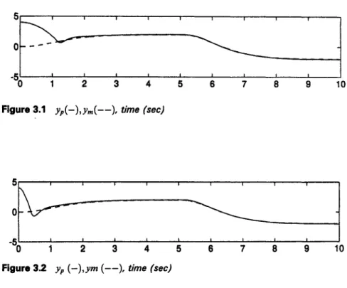
1' ' I 0 I I I ' I I I ' ._1~ I I I , I "o 1 2 3 4

Figure 3.1 yp ( - ) , Ym ( - - ) , time (sec)

I I ,I I I 5 6 7 8 9 10 i

% I '

'

" ' ; + I I ' I I ... I ... i'' I , I I I I I I 3 4 5 6 7 8 9 10

Figure 3.2 yp ( - ) , y m ( - - ) , time (sec)

all the theoretical results and corresponding claims. All the cases will assume that there are initial output error yp(0) -ym(O) = 4.

(1) In the first case, we arbitrarily choose the initial control parameters as 0j(0) = 0.1, j = 1 , . . . , 6

B/(0) = 0.1, j = l , 2

and set all the adaptation gains 7j = Oj = 0.1. As shown in Figure 3.1 (the time trajectories of yp and Ym), the global stability, robustness, and asymptotic tracking performance are achieved.

(2) In the second ease, we want to demonstrate the effectiveness of a proper choice of Oj(O) and /3j(0) and repeat the previous simulation case by increasing the values of the controller parameters to be

Oj(O)= l, j = l , . . . , 6 / 3 j ( 0 ) = l , j = 1 , 2

The better transient and tracking performance between yp and Ym can now be observed in Figure 3.2.

(19)

i I i , L - 50 ₃' ... ₄, ,, I ! I I I , I , , , l , , I , 5 6 7 8 i , I , , 9 10

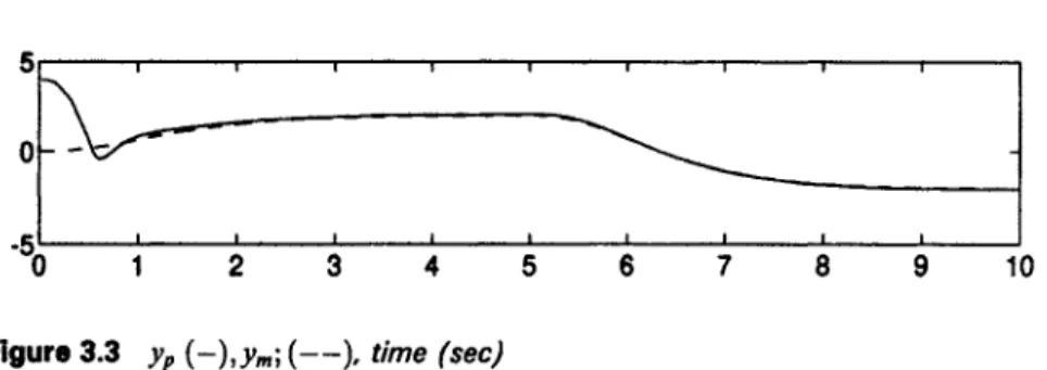
Figure 3.3 yp (-), Ym; ( - - ) , time (sec)

(3) As commented in Remark 3.2, if there is no easy way to estimate the suitable initial control parameters 0j(0) and ~.(0) like those in the second simulation case, it is suggested to use large adaptation gains in order to increase the adaptation rate of control parameters such that the nice transient and tracking performance as described in case 2 can be retained to some extent. Hence, in this ease, we use the initial control parameters as in case 1 but set all the adaptation gains to 7 j = g j = 1. The expected results are now shown in Figure 3.3, where rapid increase of control parameters do lead to satisfactory transient and tracking performance.

3.6 Conclusion

In this chapter, a new adaptive variable structure scheme is proposed for model reference adaptive control problems for plants with unmodelled dynamic and output disturbance. The main contribution of the chapter is the complete version of adaptive variable structure design for solving the robustness and performance of the traditional MRAC problem with arbitrary relative degree. A detailed analysis of the closed-loop stability and tracking performance is given. It is shown that without any persistent excitation the output tracking error can be driven to zero for relative degree-one plants and driven to a small residual set asymptotically for plants with any higher relative degree. Furthermore, under suitable choice of initial conditions on control parameters, the tracking performance can be improved, which are hardly achievable by the traditional MRAC schemes, especially for plants with uncertainties.

(20)

Appendix

Lemma A Consider the controller design in Theorem 3.1 or 4.1. If the control parameters

Oj(t),j

= 1,... ,2n,/31(t) and/32(0 are uniformly bounded Vt, then there exists #* > 0 such that

up(t)

satisfies

II(+)tlloo -< ~ll(e0)tlloo + ~ (A.1) with some positive constant ~ > 0.

Proof

Consider the plant (.3.1) which is rewritten as follows:

y(t) - do(t) =

P(s)(1 +

#Pu(s))[up](t)

(A.2)

Let f(s) be

the Hurwitz polynomial with degree n - p such that

f(s)e(s)

is proper, a n d hence,

f - l (s)p-l (s)

is proper stable since

e(s)

is minimum phase by assumption (A3). Then

y(t) - do(t) = P(s)f(s)f-l(s)(1 + #Pu(s))[ur](t )

(A.3) which implies that

f-l(s)p-l(s)[y - do](t) - #f-l(s)Pu(s)[up](t) = f-l(s)[up](t) ~u(t)*

(A.4)

Sincef-l(s)P-l(s) andf-l(s)Pu(s)

are proper or strictly proper stable, we can find by small gain theorem [7] that there exists/t* > 0 such that

IlCu*)tlloo -< ~llCrp),lloo + ~ -< ~llCe0),lloo + ~ (A.5) for some suitably defined ~ > 0 and for all # E [0, #*]. Now if we can show that

**I1(+),11oo -< ll(u*),lloo +**

(A.6)

for some ~ > 0, then (A.1) is achieved. By using Lemma 2.8 in [19], the key point to show the boundedness between u e and u* in (A.6) is the growing behaviour of signal u e. The above statement can be stated more precisely as follows: if up satisfies the following requirement

lup(tn)l >

clup(tl +

T)I

(A.7)

where tl and tl + T are the time instants defined as

[ti, tl + T] C f~ = {t i I+1 = (m.8) and c is a constant E (0, 1), then up will be bounded by u*, i.e. (A.6) is achieved. Now in order to establish (A.7) and (A.8), let

(Ap, B,, Cp)

and (A,B) be the

a(s)

(21)

define S = [x~, w~, w~,m] T. Then, using the augmented system

~p ,4p 0 0 0 x~ B~up

fvl 0 A 0 0 w] + Bup

fr = BCp 0 A 0 w2 Bdo

0 0 0 - 6 0 m 611upl+l

Since do is uniformly bounded, we can easily show according to the control design (3.16) or (3.24) that there exists ~ such that

ISI < ~ll(S),ll~ +

This means that S is regular [21] so that xr, wl, w2,m, yp and up will grow at most exponentially fast (if unbounded), which in turn guarantees (A.7) and (A.8) by Lcmma 2.8 in [19]. This completes our proof. Q.E.D.

References

[1] Chien, C. J. and Fu, L. C., (1992) 'A New Approach to Model Reference Control for a Class of Arbitrarily Fast Time-varying Unknown Plants', Automatica, Vol. 28, No. 2, 437-440.

[2] Chien, C. J. and Fu, L. C., (1992) 'A New Robust Model Reference Control with Improved Performance for a Class of Multivariable Unknown plants', Int. J. of Adaptive Control and Signal Processing, Vol. 6, 69-93.

[3] Chien, C. J. and Fu, L. C., (1993) 'An Adaptive Variable Structure Control for a Class of Nonlinear Systems', Syst. Contr. Lett., Vol. 21, No. 1, 49-57.

[4] Chien, C. J. and Fu, L. C., (1994) 'An Adaptive Variable Structure Control of Fast Time-varying Plants', Control Theory and Advanced Technology, Vol. 10, No. 4, part I, 593-620.

[5] Chien, C. J., Sun, K. S., Wu, A. C. and Fu, L. C., (1996) 'A Robust MRAC Using Variable Structure Design for Multivariable Plants', Automatica, Vol. 32, No. 6, 833-848.

[6] Datta, A. and Ioannou, P. A., (1991) 'Performance Improvement versus Robust Stability in Model Reference Adaptive Control', Proc. CDC, 748-753.

[7] Desoer, C. A. and Vidyasagar, M., (1975) Feedback Systems: Input-Output Properties, Academic Press, NY.

[8] Filippov, A. F., (1964) 'Differential Equations with Discontinuous Right-hand Side', Amer. Math. Soc. Transl., Vol. 42, 199-231.

[9] Fu, L. C., (1991) 'A Robust Model Reference Adaptive Control Using Variable Structure Adaptation for a Class of Plants', Int. J. Control, Vol. 53, 1359-1375. [10] Fu, L. C., (1992) 'A New Robust Model Reference Adaptive Control Using

Variable Structure Design for Plants with Relative Degree Two', Automatica, Vol. 28, No. 5, 911-926.

[11] Hsu, L. and Costa, R. R., (1989) 'Variable Structure Model Reference Adaptive Control Using Only Input and Output Measurement: Part 1', Int. J. Control, Vol. 49, 339-419.

(22)

[12] Hsu, L., (1990) 'Variable Structure Model'Reference Adaptive Control (VS- MRAC) Using Only Input Output Measurements: the General Case', IEEE Trans. Automatic Control, Vol. 35, 1238-1243.

[13] Hsu, L. and Lizarraide, F., (1992) 'Redesign and Stability Analysis of I/O VS- MRAC Systems', Proc. American Control Conference, 2725-2729.

[14] Hsu, L., de Araujo A. D. and Costa, R. R., (1994) 'Analysis and Design of I/O Based Variable Structure Adaptive Control', IEEE Trans. Automatic Control, Vol. 39, No. 1.

[15] Ioannou, P. A. and Tsakalis, K. S., (1986) 'A Robust Direct Adaptive Control', IEEE Trans. Automatic Control, Vol. 31, 1033-1043.

[16] Ioannou, P. A. and Tsakalis, K. S., (1988) 'The Class of Unmodeled Dynamics in Robust Adaptive Control', Proc. of American Control Conference, 337-342. [17] Narendra, K. S. and Valavani, L., (1978) 'Stable Adaptive Controller Design-

Direct Control', IEEE Trans. Automatic Control, Vol. 23, 570-583.

[18] Narendra, K. S. and Annaswamy, A. M., (1987) 'A New Adaptive Law for Robust Adaptation Without Persistent Excitation', IEEE Trans. Automatic Control, Vol. 32, 134-145.

[19] Narendra, K. S. and Valavani, L., (1989) Stable Adaptive Systems, Prentice-Hall. [20] Narendra, K. S. and B6skovi~, .1. D., (1992) 'A Combined Direct, Indirect and Variable Structure Method for Robust Adaptive Control', IEEE Trans. Automatic Control, Vol. 37, 262-268.

[21] Sastry, S. S. and Bodson, M., (1989) Adaptive Control: Stability, Convergence, and Robustness, Prentice-Hall, Englewood Cliffs, NJ.

[22] Sun, J., (1991) 'A Modified Model Reference Adaptive Control Scheme for Improved Transient Performance', Proc. American Control Conference, 150-155. [23] Wu, A. C., Fu, L. C. and Hsu, C. F., (1992)'Robust MRAC for Plants with

Arbitrary Relative Degree Using a Variable Structure Design', Proc. American Control Conference, 2735-2739.

[24] Wu, A. C. and Fu, L. C., (1994) 'New Decentralized MRAC Algorithms for Large- Scale Uncertain Dynamic Systems', Proc. American Control Conference, 3389-3393.

Adaptive variable structure control