國立臺灣大學電機資訊學院電機工程學系 碩士論文
Department of Electrical Engineering
College of Electrical Engineering and Computer Science
National Taiwan University Master Thesis
圖的接觸表示法
Contact Representations of Graphs
張以潤 Yi-Jun Chang
指導教授:顏嗣鈞博士 Advisor: Hsu-Chun Yen, Ph.D.
中華民國 104 年 6 月
June, 2015
謝
此篇論文記述了我大學四年級以來至今一部分的研究成果,其中 部分內容是基於發表於 GD'13、COCOA'14、及 WADS'15 的三篇會 議論文。本論文之所以能夠完成,首要感謝顏嗣鈞老師的指導。最 初顏老師讓我看的兩篇關於 rectilinear duals 的文章開啟了我對這個 議題的興趣,也進而造就了這一系列的研究成果。在這過程中,除 了研究上的討論與指導,顏老師也給我研究助理津貼及參加會議的 旅費,並讓我很自由地抉擇研究的方向。
我亦得感謝作為口試委員的許聞廉老師、呂學一老師、于天立老 師和陳和麟老師。老師們在口試過程中提供了許多建議與指導,讓 本篇論文更加完備。此外,我要特別感謝許聞廉老師以及張震華老 師,他們充實的圖論課程讓我培養出扎實的基礎能力。如果沒有這 些課程的練習,我的研究可能不會那麼順利。我也要特別感謝于天 立老師,因為是于老師的計算機概論課程啟發了我對於計算機科學
(特別是演算法方面)的興趣。
學術研究領域以外,我想感謝我在其他圈子的朋友及同好,你們 的存在讓我在做研究之餘也能過著充實且有趣的生活。我也必須感 謝我的家人多年來對我的關愛、支持、自由與包容。
最後,感謝正在閱讀這篇論文的你。希望此篇論文能傳達出我對 於研究的熱誠以及這領域的有趣之處。祝你閱讀愉快!
中文 要
圖 (graph) 是個常見的數學模型,能描述各種複雜的科學和工程 問題。圖形繪製 (Graph drawing) 是將一個圖表示在二維或三維空間 的過程,讓圖的結構以易於理解的方式呈現出來。由於這議題的重 要性,圖形繪製已成為計算機科學中一個快速成長的新興領域。
在眾多圖形繪製的問題中,圖的接觸表示法 (contact representa- tions of graphs) 在近年來受到的關注不斷提升。給定一個圖,它的接 觸表示法即是將圖中的各個節點對應到二維或三維空間的幾何物件,
其中任兩個節點在圖上相鄰若且唯若他們對應的物件互相接觸。
在許多接觸表示法中,rectilinear dual 是一個經典的繪製風格,能 應用於大型積體電路的布圖規劃。在該繪製風格中,圖中的各個節 點用正交多邊形來表示,多邊形的相鄰對應於節點在圖中的相鄰關 係,並且所有的多邊形合起來恰好成為一個長方形。
在本論文的前半,我們探討如何在多邊形形狀被限制的情形下設 計 rectilinear dual。因凸形 (convex shapes) 傾向比非凸形來得好看且 單純,我們提出並探討一個新的圖形繪製風格 - orthogonally convex drawing,研究如何設計 rectilinear dual 的演算法使得其中的幾何物件 皆為正交凸多邊形 (orthogonally convex polygons)。另外,為了瞭解 各形狀在繪製 rectilinear dual 中的功用與限制,我們探討可用形狀被 限制下的 rectilinear dual。我們算出⊤-free rectilinear dual 的多邊形複
雜度,驗證了⊤ 形是最有用的八邊形之直覺。
在本論文的後半,我們探討如何將 rectilinear dual 延伸及推廣到 二維正交以外的情境上。為了容納凸多邊形 (convex polygons),我們 提出並探討一個新的圖形繪製風格 - convex polygonal dual。針對這 項繪製風格,我們提出一些新的技術及 fixed-parameter tractability 的 結果。為了容納正交多面體 (orthogonal polyhedra),我們提出並探討 一個新的圖形繪製風格 - 3D floorplan。我們證明了所有 chordal graph 都能畫成 3D-floorplan。我們的畫法不但只需用到兩層,也能夠實現 任意對其中多面體指定的體積。
總體來說,在圖的接觸表示法之框架下,本論文提供了許多新的 技術及觀點。希望這篇論文指引出的研究方向能讓我們對這個充滿 挑戰性的領域有更全面的認識。
關鍵詞: 圖形繪製, 接觸表示法, 平面圖, 示意地圖, 平面規劃
Abstract
Graph represents one of the most popular abstract models in describing complex science and engineering problems. Graph drawing refers to the process of displaying an abstract graph in 2D or 3D, allowing the struc- ture as well as the meaning of the graph to be understood better and easier.
As a consequence, the design of graph drawing algorithms has become an emerging and fast growing research area in computer science.
Among problems of interest in the graph drawing community, the topic of contact representations of graphs has received increasing attention over the years. Given a graph, a contact representation of the graph is to map each vertex of the graph to a geometric object in 2D or 3D so that two vertices are adjacent iff their corresponding objects "touch".
A rectilinear dual, a classic drawing style which has found applications in VLSI floor-planning, requires that each vertex be drawn as a rectilinear polygon, adjacency in a graph correspond to side-contact in the drawing, and all rectilinear polygons together form a partition of a rectangle.
In the first half of the thesis, we investigate a variety of shape con- straints in rectilinear duals. As convex objects tend to be visually more pleasing, the drawing style orthogonally convex drawing is proposed and investigated. In addition, we study rectilinear duals using a restricted set of shapes, in order to understand the power and the limitation of different shapes in rectilinear duals. We determine the optimal polygonal complexity of⊤-free rectilinear dual, justifying the intuition that ⊤-shape is the most useful 8-sided polygon.
In the second half of the thesis, we study possible extensions and gen- eralizations of rectilinear duals beyond the 2D rectilinear setting. To ac- commodate convex polygons, the drawing style convex polygonal dual is proposed and investigated. We demonstrate several new techniques and fixed-parameter tractability results to deal with this drawing style. We also propose and investigate a new drawing style called 3D floorplan, using rectilinear polyhedra as building blocks. We show that every chordal graph admits a 3D-floorplan which uses only two layers and is also capable of realizing any volume-assignment to its constituent polyhedra.
In summary, the thesis provides a variety of new techniques and new perspectives within the framework of contact representations of graphs. We hope that this study could lead to a better understanding of contact graph representations - an exciting and challenging topic in graph drawing.
Keywords: graph drawing, contact representation, planar graph, cartogram, floorplan
Contents
口試委員會 定 i
謝 ii
中文 要 iii
Abstract iv
Contents vi
List of Figures ix
1 Introduction 1
2 Preliminaries 7
2.1 Graph Theoretic Preliminaries . . . 7
2.2 Tree-width and Chordal Graphs . . . 9
2.3 Rectilinear Polygons . . . 11
2.4 Separation Trees . . . 13
2.5 Sliceability and Area-universality . . . 16
2.6 Other Topics . . . 19
3 Orthogonally Convex Drawings 21 3.1 Related Works . . . 23
3.2 Terminologies . . . 24
3.3 Review of the Results of Rahman and Nishizeki . . . 25
3.4 No-bend Orthogonally Convex Drawings . . . 27
3.5 An Alternative Condition . . . 31
3.6 Flow Formulation for Bend-minimization . . . 40
3.7 Orthogonal Convexity in Rectilinear Duals . . . 47
4 Rectilinear Duals without T-shape 56 4.1 Related Works . . . 57
4.2 Lower Bound of Polygonal Complexity . . . 58
4.3 Construction of 12-sided⊤-free Rectilinear Duals . . . 60
4.3.1 Un-contracting a Separating Triangle . . . 60
4.3.2 Transferring Concave Corners . . . 64
4.4 Area-universal Drawings . . . 67
4.5 More about Staircase Polygons . . . 69
5 Convex Polygonal Duals 73 5.1 Related Works . . . 74
5.2 Terminologies . . . 74
5.3 Characterizing t-sided Convex Polygonal Duals . . . 76
5.4 Proof of Theorem 5.2 . . . 80
5.5 Fixed-parameter Tractability Results . . . 88
5.6 Exact Definition of the Formula t-V FAA . . . 92
5.6.1 t-FAA . . . 93
5.6.2 t-V FAA . . . 94
5.6.3 Remaining Formulas . . . 96
5.7 Further Applications of Our Technique . . . 100
6 Area-universal Drawings of Biconnected Outerplane Graphs 104 6.1 Terminologies . . . 104
6.2 Drawing Biconnected Outerplane Graphs . . . 105
7 3D Floorplans 112 7.1 Related Works . . . 112
7.2 The Drawing Algorithm . . . 113
8 Conclusion and Future Perspectives 121
Bibliography 126
List of Figures
1.1 Examples of drawing styles . . . 3
1.2 Realization of different area-assignments. . . 3
2.1 I-shape,-shape, ⊤-shape and Z-shape polygons . . . 11
2.2 Examples of rectilinear polygons. . . 12
2.3 A non-rotated⊤-shape rectilinear dual. . . 13
2.4 A separation tree. . . 14
2.5 Rectangular duals. . . 15
2.6 Illustration of inserting sub-drawing. . . 15
2.7 Construction of a rectilinear dual. . . 16
2.8 A rectilinear dual constructed by monotone staircase cuts. . . 17
2.9 Sliceability and one-sidedness in triangle contact representations. . . 19
2.10 The 5-cycle graph and its triangle contact representations. . . 20
3.1 Illustration of some terms about cycles and paths. . . 24
3.2 Illustration of the proof of Lemma 3.1. . . 27
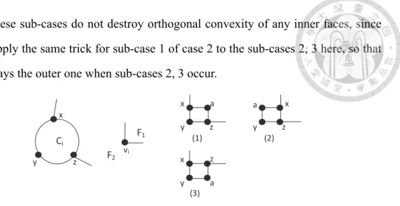
3.3 Case 1: The drawing w.r.t. a 3-legged cycle Ci. . . 30
3.4 Case 2: The drawing w.r.t. a 2-legged cycle Ci with vi a non-corner 2-vertex. . . 30
3.5 Case 3: The drawing w.r.t. a 2-legged cycle Ciwith vi a corner 2-vertex. 31 3.6 Proper and improper 2-legged cycles. . . 32
3.7 Critical paths and SGin a plane graph. . . 36
3.8 An example for Corollary 3.2. . . 39
3.9 Bend-minimized orthogonal drawings and bend-minimized orthogonally convex drawings. . . 40
3.10 Illustration of the flow network NG. . . 42
3.11 Illustration of the proof of Lemma 3.4. . . 43
3.12 Illustration of the construction of NG′. . . 46
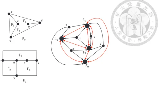
3.13 An example of a Q-floorplan. . . 47
3.14 The construction of Gprimaland the block-cutvertex tree of Gdual. . . . 49
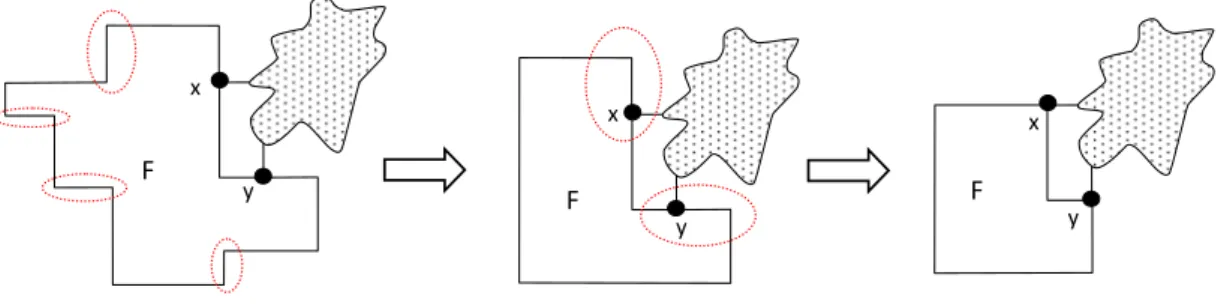
3.15 Illustration of the proof of Lemma 3.6. . . 51
3.16 Key concepts in Q-floorplanning. . . . 54
4.1 Definition of H0 and illustration of the proof of Lemma 4.1. . . 59
4.2 Location of u, v, w in the rectangular space for separating triangle{x, y, z}. 62 4.3 Illustration of un-contracting Type 1 triangles. . . 64
4.4 Illustration of un-contracting Type 2 triangles. . . 65
4.5 Illustration of transferring concave corners. . . 66
4.6 Illustration of concepts in Section 4.4. . . 67
4.7 Illustration of the proof of Theorem 4.6. . . 71
4.8 Illustration of the proof of Theorem 4.7. . . 72
5.1 Illustration of concepts introduced in Section 5.3. . . 77
5.2 Concepts in Section 5.3. . . 79
5.3 Illustration of inclusion of a new segment into a set of pseudo segments. 83 5.4 Illustration of finding ˜S. . . . 83
5.5 Illustration of relating extremal points to free vertices. . . 85
5.6 Illustration of proof of Lemma 5.2. . . 86
5.7 Illustration of the proof of Theorem 5.5. . . 92
5.8 Illustration of the proof of Theorem 5.6. . . 102
5.9 Illustration of the proof for Theorem 5.8. . . 103
6.1 A graph G and its convex polygonal dual. . . 105
6.2 The construction of an area-universal t-T4R. . . 107
6.3 Illustration of Procedures 1 and 2. . . 108
6.4 Applying P 1 to the subtree rooted at c in Fig.6.2(2). . . 110
7.1 A chordal graph G and trees T1and T2. . . 113
7.2 Illustration of a 3D floorplan. . . 115
7.3 Illustration of the removal operation . . . 117
7.4 Illustration of the insertion operation . . . 117
7.5 Illustration of the operation that changes the outer module . . . 117
7.6 Illustration of the merging operation . . . 118
7.7 Illustration of the simplified operations for interval graphs . . . 119
Chapter 1 Introduction
A graph is a mathematical structure which contains a collection of nodes and their pairwise relations. It not only has been a prime topic of study in discrete mathematics for years, but is also a natural model capturing lots of concepts and structures in computer science and electrical engineering. For instance, computer networks, social networks, circuits, and transportation routes can be modeled as graphs.
One very crucial aspect in the study of graphs is their drawings. From a practical point of view, we are frequently asked to find the best drawing of some graph occurring in real-world applications. In the floor-planning phase of the VLSI design, it is critical to find a drawing of the underlying circuit that uses a small chip area while meeting several constraints [45]; for a city having a complicated metro system, it is important to have a nicely drawn metro map that can be read and understood easily [39].
From a theoretical point of view, the investigation of various geometric represen- tations of graphs has led to profound impacts and consequences in graph theory and algorithms. On the one hand, geometry representations have inspired the introduction of some graph classes, like planar graphs and chordal graphs, among others. As they fa- cilitate the combination of graph theoretical and discrete geometric techniques, studying various concepts related to these graph classes has led to the birth of several successful branches in graph theory, like geometric graph theory and graph minor theory. On the other hand, the study of possible geometric representations of a graph class can deepen our understanding of the structures and properties of the graph class.
Basically, drawing a graph consists of three components: an input graph, a drawing style, and a quality measure. The goal of graph drawing is to search for an optimal drawing of the input graph meeting the required drawing style, where the optimality is
with respect to the designated quality measure. In many occasions, we require the input graph to be planar, as crossings are not allowed in many drawing styles.
In this thesis, we focus on one particular class of drawing styles called contact rep- resentations, where all vertices are represented by interior-disjoint geometric objects such that the adjacency relations correspond to contacts between objects. The study of contact representations can be traced back to the following well-known circle packing theorem [29]:
Every planar graph can be drawn as touching circles in the plane.
Following the above celebrated result, a variety of contact representations have been proposed and investigated over the years. Among them, the drawing style rectilinear dual has received quite a lot of research efforts in the past two decades:
A rectilinear dual is a contact representation of a graph in which each vertex corre- sponds to a rectilinear polygon, adjacency in the graph corresponds to side-contact in the drawing, and all rectilinear polygons together form a partition of a rectangle. The definition of rectilinear duals is largely motivated by the floor-planning in VLSI design.
As a result, it has not only attracted researchers in the graph drawing community [3, 4]
but has also received extensive investigation in the VLSI design community [45].
Two important quality measures for designing rectilinear duals are the following:
• Polygonal complexity: the polygonal complexity of a rectilinear dual is defined as the maximum number of sides of polygons involved in the rectilinear dual.
• Area-universality: a rectilinear dual of a graph G is called area-universal iff it can realize any area-assignment f : V (G) → R>0 in the sense that the polygon corresponding to vertex v has area f (v), v∈ V (G).
The study of area-universal drawings is motivated by the need to visualize weighted graphs. For example, a cartogram where the area of each country is scaled to its pop- ulation size is used to visualize the population of all countries in the world. Area- universality allows the visualization of any possible weight functions, and hence the
comparison of different weight functions (such as the change in population over a time period) can be visualized clearly.
A rectilinear dual can be somewhat perceived as the "dual" version of an orthogonal drawing, which is a planar drawing such that each edge is composed of a sequence of horizontal and vertical line segments with no crossings. The interplay between rectilin- ear duals and orthogonal drawings turns out to be rather useful in developing various drawing techniques, as our subsequent discussion reveals.
(1) (2) (3)
(1) (2)
(4)
A A
B B
C C
D D
Figure 1.1: Examples of drawing styles
Consider a planar graph G (drawn as a straight line drawing) in Fig. 1.1(1). Fig. 1.1(2) is a contact representation of G using touching circles. A rectilinear dual of G with its polygonal complexity being 6 is displayed in Fig. 1.1(3). Fig. 1.1(4) shows an orthog- onal drawing of G. The duality between Fig. 1.1(3) and Fig. 1.1(4) is easy to see by relating the four rectilinear regions of Fig. 1.1(3) to the four nodes in Fig. 1.1(4).
(1) (2) (3)
(1) (2)
(4)
A A
B B
C C
D D
Figure 1.2: Realization of different area-assignments.
The rectilinear dual depicted in Fig. 1.1(3) is actually area-universal. See Fig. 1.2 for its realizations of two different area-assignments: (A← 8, B ← 3, C ← 4, D ← 1) and (A← 8, B ← 4, C ← 2, D ← 2).
Following a series of recent results, an algorithm for constructing area-universal rec- tilinear duals with polygonal complexity of 8 for maximal plane graphs was proposed in [4]. This result is tight in the sense that there exists a maximal plane graph that has polygonal complexity of at least 8 in any of its rectilinear duals. Even with such match- ing lower and upper bounds in polygonal complexity, many interesting issues regarding rectilinear duals of plane graphs remain unanswered or unexplored. Specifically, in the thesis, we initiate the following two lines of research directions:
1. Imposing geometric constraints on polygons in rectilinear duals.
Most of the previous research on rectilinear duals have been focusing on the num- ber of sides of individual rectilinear polygons. Few results are available for tack- ling geometrical constraints such as orthogonal convexity or shape constraints.
To move a step further along this line of research, the following problem is inves- tigated in this thesis:
Question 1.1. Given a set of available shapes and an input graph, is it possible to design an efficient algorithm to find a rectilinear dual using only polygons of the available shapes, if it exists?
2. Extending rectilinear duals to more general settings.
In real life, it is not uncommon to encounter objects displayed as polygons which are not necessarily rectilinear. However, in contrast to the well-studied rectilinear duals, only a scarcity of results and methods are available for tackling cases for polygons that are not necessarily rectilinear. Also, motivated by the emergence of three-dimensional integrated circuits (3D ICs), the study of floor-planning in 3D should be of great interest. In light of the above, we are also concerned with the following problem in the thesis:
Question 1.2. Is it possible to design efficient algorithms to construct good floor- plans using convex polygons or 3D rectilinear polyhedra, where the quality mea- sures are area-universality and polygonal complexity?
Organization of the thesis:
Chapter 2 includes basic definitions, notations and facts that will be used throughout this thesis. We also briefly survey some existing results related to our work.
Chapters 3 and 4 are devoted to the first research direction (Question 1.1).
In Chapter 3, we focus on orthogonal convexity in rectilinear duals. A clean condi- tion for the existence of a rectilinear dual using orthogonally convex polygons subject to a given orthogonally convex boundary constraint is presented. Our new finding relies on the establishment of a close connection between the "dual" setting (i.e.,, the rectilinear dual) and its "primal" version (i.e., the orthogonal drawing) in the study of orthogonal convexity. We propose the drawing style orthogonally convex drawing which serves as the orthogonal analogue of the convex drawing. To our best knowledge, our effort here is the first time that orthogonal convexity is studied in rectilinear duals and orthogonal drawings. Part of this chapter has appeared in [9].
Motivated by an observation that most algorithms yielding rectilinear duals of low polygonal complexity require the use of⊤-shape polygons or their extensions, our aim in Chapter 4 is to justify the intuition that ⊤-shape polygons are more powerful than other 8-sided ones. To this end, it is proven that the required polygonal complexity for maximal plane graphs increases from 8 to 12 if⊤-shape polygons and their extensions are not allowed. We then continue this line of research by studying other constrained rectilinear duals. Part of this chapter has appeared in [10].
Chapters 5, 6, and 7 are devoted to the second research direction (Question 1.2).
In Chapter 5, a new drawing style called the convex polygonal dual, serving as the convex polygonal analogue of the rectilinear dual, is proposed. We give a finite combi- natorial characterization for plane graphs admitting such drawings. Our characterization not only leads to some fixed-parameter tractability results, but it can also be applied to giving quick alternate proofs for existing results and establishing relationship between rectilinear duals and convex polygonal duals. Part of this chapter has appeared in [11].
In Chapter 6, we give a detailed study of convex polygonal duals for biconnected outer plane graphs. Our study yields a clean condition for the existence of a drawing for a given polygonal complexity. A simple procedure is also given for constructing an area-universal drawing of low polygonal complexity.
In Chapter 7, rectilinear duals are generalized to 3D by representing each vertex of a graph as an orthogonal polyhedron. This study opens the door for non-planar graphs to be accommodated in a floorplan design. We prove that all chordal graphs admit such 3D drawings. This result parallels the well-known fact that all maximal plane graphs admit rectilinear duals, as chordal graphs and maximal plane graphs are regarded as the natural candidates of "triangulated graphs" in the general and the planar settings, respectively.
Finally, Chapter 8 summarizes the results reported in this thesis. Some open prob- lems are posted in this chapter as well.
Chapter 2
Preliminaries
The goal of this chapter is to introduce some basic notations and preliminary results required for the subsequent discussion. We do not intend to give a comprehensive tuto- rial for each topic we discuss, as there already exist quite a few nicely written literatures devoted to these topics.
For a more comprehensive introduction to graph drawing, the reader is recom- mended to have a look at the book [34] and the two PhD theses [1, 43]. They not only provide a nice introduction to the field, but they also contain materials intimately related to the content of the thesis. Also, the reader is referred to [44] to learn more about graph theory.
2.1 Graph Theoretic Preliminaries
Given a graph G = (V, E), we write ∆(G) to denote the maximum degree of G. We write V (G) and E(G) to denote the set of vertices and the set of edges of G, respectively.
Graph G is called a d-graph if ∆(G)≤ d.
Note that the definition of the notion G∗changes in different chapters of the thesis, and we usually do not follow the custom to use G∗to denote the dual graph of G.
A graph is simple if it contains no self-loop and no multi-edges. A multi-graph is a graph where self-loops are disallowed while multi-edges are allowed. If not otherwise stated, all graphs in the thesis are assumed to be simple.
A graph is k-connected if it contains at least k + 1 vertices, and if removal of any k−1 vertices does not render the graph disconnected. "biconnected" and "triconnected"
are synonyms for "2-connected" and "3-connected", respectively. For k = 1, we can
simply call the graph connected. If not otherwise stated, all graphs in the thesis are assumed to be connected.
A graph is planar if it can be drawn on a plane without any edge crossing. A plane graph is a planar graph with a fixed combinatorial embedding and a designated outer face FO. For any vertex and edge, we call it boundary if it is located in FO. Otherwise, it is non-boundary.
An outerplanar graph is a planar graph with a planar embedding in which all ver- tices belong to the outer face. An outerplane graph is an outerplanar graph in such an embedding.
A graph H is a subgraph of G if V (H) ⊆ V (G), E(H) ⊆ E(G). We also write H ⊆ G to denote the subgraph relation.
Given a graph G, a path P is a subgraph such that V (P ) = {v1, v2. . . , vk} and E(P ) = {{vi, vi+1}|1 ≤ i ≤ k − 1}, for some k > 1. A cycle C is a subgraph such that V (C) = {v1, v2, . . . , vk} and E(C) = {{vi, vi+1}|1 ≤ i ≤ k − 1} ∪ {{v1, vk}}, for some k > 1. For convenience, a path (or cycle) is also written as (v1, v2, . . . , vk).
Unless otherwise stated, repeated vertices are not allowed in paths and cycles in the sense that vi ̸= vj if i ̸= j.
If we write H = G\ S (or equivalently, H = G − S), where S can be a subgraph of G, a subset of V (G), or a subset of E(G), then H is the subgraph of G defined by the following procedure: (1) V (H)← V (G)− the vertices in S; (2) E(H) ← E(G)−
the edges in S; (3) removing the isolated vertices (those incident to no edge in E(H)) in H.
A cycle is Hamiltonian if it contains all vertices in the underlying graph. A graph is Hamiltonian if it has a Hamiltonian cycle.
A drawing of a planar graph divides the plane into a set of connected regions, called faces. A contour of a face F is the cycle formed by vertices and edges along the bound- ary of F . Sometimes we slightly abuse the terminology to write F to denote its contour.
Such a cycle is also called a facial cycle. The contour of the outer face FOis also denoted as CO.
Given a plane graph G, the inner (also known as internal or interior) region of a cycle C is the region enclosed by C (containing the vertices and the edges located interior of the cycle C), and the outer (also known as external or exterior) region of C is the region outside of C (containing the vertices and the edges located exterior of the cycle C). The inner and outer regions of C are written as in(C) and out(C), respectively. The edges and vertices located along C (i.e. E(C), V (C)) are neither in the inner region nor in the outer region of C. We use G(C) to denote the subgraph of G that contains exactly C and vertices and edges residing in its inner region.
2.2 Tree-width and Chordal Graphs
A tree is a connected graph without any cycle. It is a basic fact that a tree T has exactly|V (T )| − 1 edges (assuming it is simple). However, other than the trees, there are quite a few graph classes (e.g. outerplanar graphs) also having some sort of "tree structure", and the notion tree-width formalizes this concept.
A tree decomposition of a graph G is a tree T such that the following properties are satisfied:
1. V (T ) ={X1, . . . , X|V (T )|}. Each Xi represents a subset of V (G).
2. For each edge e ={u, v} ∈ E(G), there is an Xisuch that u, v ∈ Xi. 3. For each vertex v∈ V (G), there is an Xi such that v ∈ Xi.
4. If v ∈ Xi∩Xj, for all Xkin the unique path linking Xi, Xjin T , we have v∈ Xk. We denote a vertex in V (T ) as a bag instead of a vertex to avoid confusion. The width of T is defined to be max{|Xi| − 1|Xi ∈ V (T )}. The tree-width is then defined as below:
Definition 2.1. A graph G is said to have tree-width k iff a minimum width tree decom- position of G has width k.
As an example, each outerplanar graph has tree-width at most two.
A lot of difficult (NP-hard) problems have polynomial time solutions on trees, as it is usually easier to design a dynamic programming algorithm on a tree structure than on a general graph. Intuitively, graphs of bounded tree-width should share this kind of
"algorithmic advantage". The famous algorithmic meta-theorem "Courcelle's Theorem"
formalizes this intuitive idea:
Theorem 2.1 ( [13,14]). Any graph property expressible in MSO2is linear time solvable for graphs of bounded tree-width
Monadic second-order logic, a fragment of second-order logic, allows only quantifi- cation over unary relations (i.e., sets). The monadic second-order logic on graph MSO2 includes the following ingredients:
• Variables: vertices, edges, set of vertices, and set of edges.
• Relations: ∈, =, edge-vertex incidence ( ), and adjacency ( ).
• Connectives: ∨, ∧, ¬, →.
• Quantifiers: ∀, ∃ that can be applied to all kinds of variables.
Courcelle's Theorem plays an important role in Chapter 5.
For more about monadic second-order logic on graph structures, the reader is re- ferred to [14, 16].
Besides the above algorithmic application, there are still other topics in graph theory intimately relate to tree-width. A graph is chordal if each of its cycle C of length more than 3 has a chord, which is an edge e = {u, v} ̸∈ E(C) such that u, v ∈ V (C). As a result, each induced cycle in a chordal graph is necessarily a triangle.
Interestingly, chordal graphs are exactly the ones who admit a tree-decomposition where each bag is a clique, which is a subgraph H such that ∀u, v ∈ V (H), {u, v} ∈ E(H). Such a tree-decomposition is also called a clique tree. This concept is crucial in Chapter 7.
2.3 Rectilinear Polygons
A polygon is rectilinear if all its edges are parallel to x-axis or y-axis of the Cartesian coordinate system. A rectilinear polygon is also known as an orthogonal polygon. In this section we present some notations for rectilinear polygons, which are mostly applied in Chapter 3, 4 of the thesis.
Figure 2.1: I-shape,-shape, ⊤-shape and Z-shape polygons
Two rectilinear polygons are combinatorially equivalent iff they admit the same circular order of angles. When there is no need to differentiate polygons that are com- binatorially equivalent to each other, it is without loss of information to use circular order of angles to represent a rectilinear polygon. For example, rectangle (or called I-shape), -shape, ⊤-shape, W-shape, ⊔-shape, Z-shape can be represented by (V, V , V, V ), (V, V , V, C, V, V ), (V, V , C, V , V, C, V, V ), (V, V, V , C, V , C, V, V ), (V, V, V , C, C, V , V , V ), (V , V , V , C, V , V , V , C), respectively, where the letters V and C represent convex and concave corners, respectively. See Fig. 2.1 for some illustrations.
Given a sequence P of Cs and V s, we let ♯C(P ) and ♯V(P ) denote the numbers of concave and convex corners, respectively.
Here we define a partial order "≼" on rectilinear polygons as follows:
Definition 2.2. Let P and Q be two rectilinear polygons. P ≼ Q iff Q can be obtained by iteratively inserting (C, V ) or (V, C) into P .
The drawing style rectilinear dual is defined as follows:
Definition 2.3. A rectilinear dual is a contact representation of a graph meeting the below conditions:
1. Each vertex corresponds to a rectilinear polygon.
2. Adjacency in the graph corresponds to side-contact in the drawing.
3. All rectilinear polygons together form a partition of a rectangle.
Let R be a rectilinear dual, we call it Q-free iff for each polygon of shape P used in R, we have Q ̸≼ P . We remark that the partial order "≼" actually reflects the intu- itive idea of degeneracy in the way that P ≼ Q indicates that Q can degenerate to P . Therefore, the notion of "Q-freeness" captures the idea of "Q is not a degenerated form of any rectilinear polygon in the drawing".
A class of rectilinear polygons called staircase is defined as follows:
Definition 2.4. Let P be a rectilinear polygon. P is monotone staircase iff P = (a, S1, b, S2) clockwise, where a = b = V and both S1and S2consist of Cs and V s appearing alternatively and both start and end with V , where the two points a, b are exactly at the most south-western (i.e., lower left-hand) and the most north-eastern (i.e., upper right-hand) corners.
(1) (2)
a
b
Figure 2.2: Examples of rectilinear polygons.
In other words, a monotone staircase polygon is a polygon formed by two mono- tonically rising staircases, each of which is a sequence of horizontal and vertical line segments from the bottom-left corner to the top-right corner of the polygon. A staircase polygon is a rectilinear polygon resulting from rotating a monotone staircase polygon 90◦, 180◦, or 270◦.
The following facts are easy to observe, and may be explicitly or implicitly applied in the discussion throughout the thesis.
Fact 2.1. ♯V(P )− ♯C(P ) = 4 in any rectilinear polygon P .
Fact 2.2. A rectilinear polygon is orthogonally convex iff it does not contain consecutive
concave corners.
Fact 2.3. A rectilinear polygon P is staircase iff⊤̸≼ P and P is orthogonally convex.
Fact 2.4. A rectilinear polygon P satisfies⊤≼ P iff P = (S1, a, S2, b, S3, S4) such that a = b = V and ♯C(S2) = ♯V(S2), ♯C(S1)− ♯V(S1) = ♯C(S3)− ♯V(S3) = 1.
Fig. 2.2(1) is an example of a staircase polygon. The polygon in Fig. 2.2(2) can degenerate to⊤-shape by removing the two pairs of corners (circled in the picture); the reader can verify Fact 2.4 by considering its representation (C, V, V, V, C, C, V, V , V , V , C, V ) = (S1 = (C), a = V, S2 = (), b = V, S3 = (V, C, C), S4 = (V, V, V, V, C, V )).
a b
c d
F
(1.1) (1.2)
(2.1) (2.2) (2.3) (2.4)
(3) (4)
(1) (2)
Figure 2.3: A non-rotated⊤-shape rectilinear dual.
Sometimes there is a need to differentiate combinatorially equivalent polygons that have different orientations. For example, Fig. 2.3(2) shows the four possible orienta- tions of the⊤-shape. We use the term "non-rotated" to describe a situation that exactly one orientation is allowed to appear in a rectilinear dual.
Fig. 2.3 (1) is a rectilinear dual using only non-rotated⊤-shape polygons, since all the polygons are combinatorially equivalent to (and possibly a degenerate of) exactly one of the four possible⊤-shape polygons depicted Fig. 2.3(2).
A rectilinear dual using only monotone staircase polygons can be regarded as a non- rotated staircase rectilinear dual.
2.4 Separation Trees
In this section we describe an important technique to construct rectilinear duals.
b c
d f c
d
b a
b f
d i
a
d c
g
h e h
e f
c
d b
a g
i
Graph G
Figure 2.4: A separation tree.
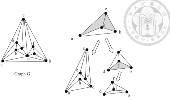
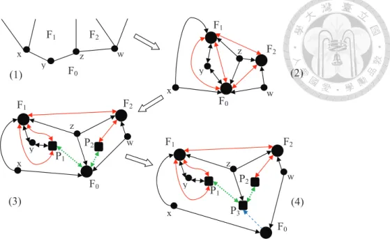
Let△ be a triangle (a cycle of length 3 in a graph). We call △ a separating triangle (also known as a complex triangle) iff G(△) ̸= △ in any planar embedding of G. G△ is defined to be the induced subgraph of the set of vertices {v ∈ V (G(△))| for any triangle△′ ̸= △ in G(△), v does not reside in the interior region of △′}. For graph G depicted in Fig. 2.4, G{a,b,c} is the subgraph induced by{a, b, c, d}. The separation tree of a maximal plane graph G is defined to be the unique rooted tree whose vertices are separating triangles and the CO of G, with △ being a descendant of △′ iff △ is contained in G(△′). See Fig. 2.4. The reader is referred to [43] for a more detailed introduction to separation trees.
The contraction of a triangle△ is an operation that replaces G(△) with △; the un- contraction of a (previously contracted) triangle△ is an operation that replaces △ with G△. The descendants of△ remain contracted when we un-contract △.
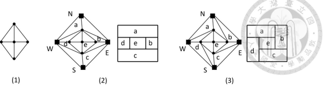
A rectangular dual is a rectilinear dual in which each polygon corresponding to a vertex is a rectangle. The following theorem gives a clean characterization of graphs admitting such a drawing [30]:
Theorem 2.2 ( [30], and see also [19]). An internally triangulated plane graph G admits a rectangular dual iff we can augment G with four vertices{N, E, S, W } satisfying:
1. The new outer face is the quadrangle{N, E, S, W };
(1) (2) (3) a
S
a b b
c c
d e d e e
a b d c
d e b a
c
S
E
W E W
N N
Figure 2.5: Rectangular duals.
2. The resulting graph is internally triangulated and contains no separating triangle.
Fig. 2.5(2,3) show two rectangular duals for the graph in Fig. 2.5(1) corresponding to the augmentation of{N, E, S, W } depicted.
s
t r
s
t r
Figure 2.6: Illustration of inserting sub-drawing.
The tight connection between separating triangles and rectangular duals makes sep- aration trees particularly useful in constructing rectilinear duals. A general framework for building rectilinear duals based on separation trees is sketched as follows:
1. Let△1,△2, . . . ,△kbe a level-order traversal of the separation tree. We let G′ =
△1(CO, the outer triangle).
2. Construct a rectangular dual of G′ as the initial drawing.
3. For i = 1 to k, we un-contract△i, and plug-in the rectangular dual of G△i \ △i
to the current drawing.
See Fig. 2.6 for a conceptual illustration of inserting rectangular dual of G△i\ △i
when△i = {s, t, r} is un-contracted. Note that such an insertion inevitably add some
concave corners to nearby polygons, as a result, if a graph contains a separating triangle, its polygonal complexity must be at least 6 in any of its rectilinear dual. The reader is referred to [43,45] for a more comprehensive treatment to the approach. See Fig. 2.7 for a full example of a top-down construction of a rectilinear dual based on this approach.
The above framework is adapted in Chapter 4. The "primal version" of the above method is used in Chapter 3.
u v w
x
z y c
wc u
v x
y z c
x
y z x
y z
x
y z
c x
z y
Figure 2.7: Construction of a rectilinear dual.
2.5 Sliceability and Area-universality
In this section we present two important aspects of rectangular duals: sliceability and area-universality. Recall that a rectangular dual is a rectilinear dual where all its polygons are rectangles. These concepts can be generalized or extended to other set- tings, and this plays an important role in our later discussion.
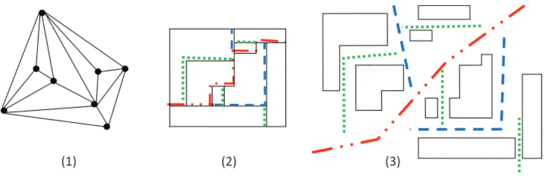
A rectangular dual is said to be sliceable if it can be obtained by recursively cutting a rectangle into two parts by a horizontal or a vertical line. Sliceable rectangular duals enjoy certain nice properties, facilitating global routing by taking advantage of the hi- erarchical structure of partitioning by the cut lines, for instance. Also see [26] for an application of sliceable rectangular duals in graph drawing.
See Fig. 2.5(2) for an example of a sliceable rectangular dual; and see Fig. 2.5(3) for an example of a non-sliceable rectangular dual.
As a generalization of sliceability in floor-planning, monotone staircase cuts have
been proposed (see, e.g., [25, 32]), which are able to yield a richer set of floorplan structures while retaining certain attractive properties enjoyed by sliceable floorplans.
In fact, floorplans using monotone staircase polygons are exactly those that can be ob- tained using monotone staircase cuts. This kind of floorplan is investigated in Chapter 4.
See Fig. 2.8(2,3) for an example.
(1) (2) (3)
Figure 2.8: A rectilinear dual constructed by monotone staircase cuts.
A rectangular dual (or a rectilinear dual) is area-universal if it can realize any area- assignment f : V (G)→ R>0in the sense that each polygon P corresponding to vertex v has area f (v). One seminal result regarding area-universal rectilinear duals is the following:
Theorem 2.3 ( [4]). For any maximal plane graph, there is an area-universal rectilinear
dual of polygonal complexity 8 using only non-rotated⊤-shape polygons.
This result is tight in the sense that there exists a maximal plane graph where all its rectilinear duals have polygonal complexity of at least 8. However, given a recti- linear dual, currently there is no easy way to decide whether it is area-universal or not.
Moreover, even if the rectilinear dual is known to be area-universal, there is no known combinatorial algorithm to realize a given area-assignment.
There are a few positive results for area-universal rectangular duals in literatures.
For example, area-universality can be characterized by one-sidedness [19]:
Theorem 2.4 ( [19]). A rectangular dual is area-universal iff it is one-sided.
A rectangular dual is one-sided iff for each straight line in the drawing, one side of it borders exactly one polygonal region. The two rectangular duals in Fig. 2.5 are both one-sided (and hence area-universal).
More interestingly, the aforementioned concepts seem to be able to extend to other settings beyond rectangular duals and rectilinear duals.
Definition 2.5 ( [21, 28]). A proper touching triangle representation is a contact repre-
sentation of a graph meeting the below conditions:
1. Each vertex corresponds to a triangular region.
2. Adjacency in the graph corresponds to side-contact in the drawing.
3. All triangular regions together form a partition of a triangle.
Let △ = {a, b, c} be a triangle. We define the following two operations which subdivide△:
1. Adding a new point d inside of△, followed by adding three straight lines linking d to a, b, c.
2. Adding a new point d dividing the line bc, followed by adding a straight line linking a to d.
We call a proper touching triangle representation sliceable iff it can be constructed by applying the above 2 operations to its constituent triangles recursively. A proper touching triangle representation is one-sided iff for each straight line in the drawing, one side of it borders exactly one polygonal region. Following basic geometry, the following lemma is easy to observe:
Lemma 2.1. Every one-sided and sliceable proper touching triangle representation is area-universal. Moreover, if the coordinates of the 3 boundary vertices are fixed, the drawing realizing any given area-assignment is unique.
(1) G
B A
F
E D C
(2) a
b c
d
f e g
h i j A C
D G E
B F
A B C
D
(1) (2) (3)
Figure 2.9: Sliceability and one-sidedness in triangle contact representations.
See Fig. 2.9 for illustrations for the above concepts. Fig. 2.9(1) is one-sided but not sliceable; Fig. 2.9(2) is one-sided and sliceable; and Fig. 2.9(3) is not one-sided but sliceable. Note that Fig. 2.9(3) is clearly not area-universal since it cannot realize the area-assignment: f (A) = f (C) = 0.4, f (B) = f (D) = 0.1.
See [20] for an interesting result on area-universal drawing in a non-rectilinear set- ting. They prove the area-universality of their contact representation by refining the drawing to triangles, which are easier to deal with.
Lemma 2.1 is applied in Chapter 6. Sliceability and area-universality are highly relevant to Chapter 4.
2.6 Other Topics
In this section we give a very short introduction to some topics that are important but omitted in the previous sections. For each topic, several good references are provided for interested readers to learn more about them.
Matchings and Flows. In many situations, a graph drawing problem can be reduced to a flow or a matching problem. In these cases, the essential information required in constructing the desired drawing, like the number of bends in each edge and the de- gree of the angle for each vertex in a face, can be encoded using a matching or a flow.
See Section 6.2, 8.2 of [34] for the classic applications of this technique to orthogonal drawings and rectangular drawings, which are the "primal version" of rectilinear duals and rectangular duals, respectively. See [12, 33, 40, 41, 45] for more. This technique is
applied in Chapter 3.
Schnyder Labelings. Undoubtedly, Schnyder Labeling [38] is one of the most suc- cessful techniques in graph drawing, and it is especially useful in dealing with contact representations. Basically, a Schnyder Labeling is a labeling of corners of a maximal plane graph to{1, 2, 3} meeting some conditions. This technique was originally used to construct a straight line drawing in a small grid (see [38] and Chapter 4 of [34]). Since then, it has found applications in varieties of contact representations (see [3, 4, 31] for instances).
Triangular Drawings and Contact Representations. In contrast to the well-studied rectangular duals and rectilinear duals, only a scarcity of results were available in non- rectilinear settings, as it is mathematically easier to handle rectilinear things. Most of the studies in non-rectilinear setting are centered on triangles. The investigation of proper touching triangle representations has been reported in two recent articles [21,28].
Touching triangle representations without boundary constraints have been studied in [22]. In the primal setting, straight line triangle representation was proposed and stud- ied in [1, 2]. See Fig 2.10 for a showcase of some triangle contact representations: (1) the 5-cycle, (2) a point-side triangle contact representation, (3) a touching triangle repre- sentation without any boundary constraint, (4) a proper touching triangle representation, and (5) a touching triangle representation with a convex polygon boundary.
Figure 2.10: The 5-cycle graph and its triangle contact representations.
Chapter 3
Orthogonally Convex Drawings
Both straight line drawing and orthogonal drawing are very well-studied graph drawing styles (see Fig. 1.1); and convexity is a very important aspect in drawing graphs [34]. However, in contrast to the well-studied convex drawing, which is a straight line drawing plus a requirement that each face is drawn as a convex polygon, we know very little about convexity in orthogonal drawing.
Of course, one may simply regard the so-called rectangular drawing (an orthogonal drawing where all faces are drawn as rectangles) as the "convex drawing" for orthogonal drawing, since the rectangles are exactly the convex orthogonal polygons. However, this drawing style seems to be too limited. As the following theorem shows, not really many graphs enjoy such a drawing:
Theorem 3.1 ( [42]). Given a plane graph G with four designated vertices on CO(G), it admits a rectangular drawing with the four designated vertices being the four corner of the outer rectangle iff:
1. every 2-legged cycle contains at least two designated vertices, and 2. every 3-legged cycle contains at least one designated vertex.
We note that 3-legged cycles are the "primal" counterpart of the separating triangles, which we present in Section 2.4.
In a plane graph G, an edge e = {u, v} ̸∈ E(G(C)) is called a leg of C if at least one of the two vertices u and v belongs to C. The vertices in V (C) that are incident to some leg of C are called the legged-vertices of C. C is k-legged if C has exactly k legged-vertices. In a biconnected plane 3-graph, each legged-vertex of C is incident to exactly one leg of C.
As a result, we suggest that orthogonal convexity is a more suitable candidate for studying convexity in orthogonal drawings than the traditional convexity.
In view of the above, in this chapter, we study orthogonal convexity in both orthog- onal drawings and rectilinear duals.
To be more specific, our contributions are:
1. The drawing style orthogonally convex drawing is proposed. A necessary and sufficient condition, along with a linear time testing algorithm, is presented for biconnected plane 3-graphs to admit a no-bend orthogonally convex drawing.
2. We then present an alternative characterization for no-bend orthogonally convex drawings of biconnected plane 3-graphs. It allows us to prove the following re- sults:
• For any triconnected plane 3-graph, the minimum number of bends remains the same regardless of whether the drawing is orthogonally convex or simply orthogonal.
• For any subdivision of a triconnected plane 3-graph, its orthogonally convex drawing requires at most one more bend than its orthogonal counterpart.
3. Also based on the above alternative characterization, a flow network algorithm, running in O(n1.5log3n) time, is devised for the bend-minimization problem for biconnected plane 3-graphs.
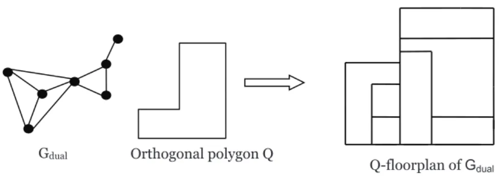
4. Lastly, we apply our analysis of orthogonally convex drawings to characteriz- ing internally triangulated graphs that admit the so-called Q-floorplans, which are rectilinear duals using only orthogonally convex polygons such that the outer boundary is an orthogonally convex polygon combinatorially equivalent to a given orthogonally convex polygon Q.
3.1 Related Works
The bend-minimization problem, a classical optimization problem in orthogonal drawings, is to minimize the total number of bends in the drawing. The problem is NP-complete in the most general setting, i.e., for planar graphs of maximum degree 4 [23].
Several subclasses of graphs are known to have polynomial time algorithm to find a bend-minimized orthogonal drawing, including planar graphs of maximum degree 3, series-parallel graphs, and graphs with fixed embeddings [6, 41].
Several attempts have been made to extend the model of orthogonal drawings to bet- ter comply with various requirements in practical applications. For example, to improve the readability and aesthetic feel, a new model called the slanted orthogonal drawing was introduced in [7]. In this model, a 90◦ bend is replaced by two 135◦ bends to smoothen the edges. To allow graphs of degree more than 4 to be drawn, the so-called quasi-orthogonal drawing model was invented in [27].
The current approaches for computing orthogonal drawings can be roughly divided into two categories, one uses flow or matching to model the problem (e.g., [6, 12, 41]), while the other tackles the problem in a more graph-theoretic way by taking advantage of structural properties of graphs (e.g., [35--37]). The former usually solves a more general problem, but often requires higher time complexity. On the contrary, algorithms in the latter focus on specific kinds of graphs, resulting in linear time complexity in many cases.
As we shall see in our subsequent discussion, the technique used in this chapter involves a mixture of the above two types of strategies.
For other perspectives of orthogonal drawings, the reader is referred to [18] for a survey chapter.
3.2 Terminologies
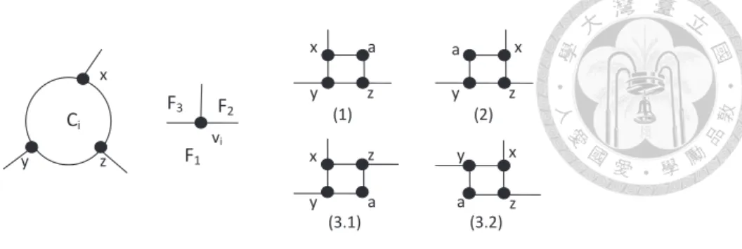
For any path, cycle, and face, we call it boundary iff it shares some edges with CO. A contour path P of a cycle C is a subpath of C such that P includes exactly two legged-vertices x and y of C, and x and y are the two endpoints of P . Therefore, each k-legged cycle has exactly k contour paths. If a contour path intersects (i.e., shares some edges with) the outer cycle, we call it boundary contour path. In fact, each boundary contour path is a subpath of CO. Each contour path P of C is incident to exactly one face, denoted as FC,P, in the outer region of C.
z
y x
u v x
y
z
y F
F x
a
b x
u F2
F0
v
t s y a
b
c
q
r
F1
i
k
h
j w k
g k m
k z
Figure 3.1: Illustration of some terms about cycles and paths.
See Fig. 3.1 for an example. Consider two cycles C1 = (s, t, u, v) and C2 = (x, b, i, a, z, y, c) (both drawn in bold line). C1 is a non-boundary 2-legged cycle, of which two legged-vertices are t and v, and two legs are (t, q) and (v, r). C1 is also a facial cycle, which is the contour of F1. C2is a boundary 3-legged cycle, of which three legged-vertices are x, y, and z. P1 = (t, u, v) is a contour path of C1. P2 = (z, a, i, b, x) is the boundary contour path of C2. We have FC1,P1 = F2and FC2,P2 = F0.
Let D(G) be an orthogonal drawing of the plane graph G with outer cycle CO. Given a cycle C, we use D(C) (or equivalently D(F ) if C is the contour of a face F ) to denote the drawing of C in D(G).
The orthogonally convex drawing is defined as follows:
Definition 3.1. D(G) is an orthogonally convex drawing of G if D(F ) is an orthogo- nally convex polygon for each face F other than the outer one.
In an orthogonal drawing D(G), angC(v) denotes the interior angle of v in polygon D(C). We call v a convex corner, non-corner, and concave corner of C if angC(v) is 90◦, 180◦, and 270◦, respectively. A corner in the drawing D(G) is either a bend on some edge, or a vertex v of G such that angC(v)̸= 180◦for some C. If v is a non-corner of C, v is on a side of the polygon D(C).
Given a face F surrounded by its contour cycle C in a drawing D, we use nextF(v) to denote the first corner after v in the counter-clockwise orientation of C; similarly, prevF(v) is defined to be the first corner after v in the clockwise orientation.
Fact 3.1. Let v be a non-corner vertex in the common boundary of two faces F and H in an orthogonal drawing. If nextF(v) is concave, prevH(v) must be convex.
From Section 3.3 to Section 3.6, graphs under the name G are assumed to be bicon- nected,△(G) ≤ 3, and may have multi-edges.
3.3 Review of the Results of Rahman and Nishizeki
Among existing results concerning orthogonal drawings, Rahman et al. [36] gave a necessary and sufficient condition for a biconnected plane 3-graph to admit a no-bend orthogonal drawing, and they devised an algorithm to test the condition, and subse- quently constructed such a drawing if one exists.
Theorem 3.2 ( [36]). A biconnected plane 3-graph G has a no-bend orthogonal draw- ing iff G satisfies the following three conditions:
(1) There are four or more 2-vertices (i.e., vertices of degree 2) of G on CO(G).
(2) Every 2-legged cycle contains at least two 2-vertices.
(3) Every 3-legged cycle contains at least one 2-vertex.
Theorem 3.2 obviously holds even when G has multi-edges, as such graphs do not have no-bend orthogonal drawings.
The drawing algorithm in [36] performs the following steps recursively: (1) reduc- ing the original graph G into a structurally simpler graph G∗by collapsing the so-called
"bad cycles", (2) drawing G∗ in a rectangular fashion, and (3) plugging in the orthog- onal drawings of those bad cycles to the rectangular drawing of G∗ to yield a no-bend orthogonal drawing of G.
The reader can imagine it as a "primal version" implementation of the general frame- work for building rectilinear duals based on separation-trees described in Section 2.4.
Algorithm( [36]). No-bend-Orthogonal-Draw(G)
1. Determine four 2-vertices on CO(G) as designated corners.
2. Find the maximal bad cycles C1, C2, ..., Ckin G.
3. For each i, 1≤i≤k, contract cycle Ci to a single vertex vi. 4. Let G∗ be the resulting graph.
5. Find a rectangular drawing D(G∗) by Rectangular-Draw such that the four des- ignated corners are the corners of the bounding rectangle.
6. For each i, 1≤i≤k, extend each viin D(G∗) to an appropriate rectangular region, and then patch D(G(Ci)) (using the outcome of calling No-bend-Orthogonal- Draw(G(Ci))) to D(G∗) by identifying the four designated corners of G(Ci) to the corners of the rectangle region.
7. Return the resulting drawing as D(G).
Algorithm Rectangular-Draw computes the rectangular drawing of an input graph meeting the conditions in Theorem 3.1.
A key in Algorithm No-bend-Orthogonal-Draw above is the identification of a certain type of cycles called bad cycles. Bad cycles are cycles that are 2-legged or 3-legged if the four designated corner vertices in CO are considered as leg-vertices.
Intuitively, bad cycles are cycles that violate the conditions under which a graph admits
a rectangular drawing. For instance, consider the graph in Fig. 3.1. If {h, i, j, k} are the 4 designated vertices, then (w, z, a, i, b, x, c, y) (a 3-legged cycle as i is considered a legged-vertex) is a bad cycle, whereas (r, v, u, t, q, j, g, h) (a 4-legged cycle including legged-vertices h and j) is not a bad cycle. Maximal bad cycles are bad cycles that are not contained in G(C) for any another bad cycle C. Note that whenever Rectangular- Draw is called for G∗ in procedure No-bend-Orthogonal-Draw, G∗ (with each of the maximal bad cycles contracted to a single vertex) always meets the condition for the existence of a rectangular drawing.
The reader is referred to [36] for more.
3.4 No-bend Orthogonally Convex Drawings
Our goal in this section is to give a necessary and sufficient condition for bicon- nected plane 3-graphs to have no-bend orthogonally convex drawings, in a way similar to Theorem 3.2.
Figure 3.2: Illustration of the proof of Lemma 3.1.
Lemma 3.1. Consider a no-bend orthogonally convex drawing D(G) of a plane graph G. For every 2-legged cycle C with legged-vertices x and y and a contour path P of C, the number of convex corners of D(C) in V (P )\ {x, y} must be at least 1 more than that of concave corners, if either
(1) C is a boundary cycle and P is its boundary contour path, or
(2) C is non-boundary and P is any of its contour paths.
Proof. The result is proven by contradiction. Suppose there exists a contour path P of a cycle C falsifying the lemma. Let P′ be the other contour path of C. Clearly P′ is a non-boundary contour path, and hence FC,P′ is an inner face. Since the number of convex corners in V (P )\ {x, y} of D(C) is no more than that of the concave corners, to have the total number of convex corners in C 4 more than that of the concave corners (in view of Fact 2.1), the number of convex corners in V (P′)\ {x, y} of D(C) must be at least 2 more than that of concave corners.
In other words, the number of concave corners in V (P′)\ {x, y} of D(FC,P′) is at least 2 more than that of convex corners. Therefore, there exist consecutive con- cave corners in the contour of FC,P′, so D(FC,P′) is not orthogonally convex (Due to Fact 2.2), contradicting the assumption that D(G) is orthogonally convex.
See Fig. 3.2 for an illustration. As the number of convex corners in V (P )\ {x, y}
is no more than that of the concave corners, there are two consecutive concave corners in FC,P′, which are u and v in the figure.
We are now in a position to present the main result of the section.
Theorem 3.3. A biconnected plane 3-graph G admits a no-bend orthogonally convex drawing iff the three conditions (1), (2) and (3) in Theorem 3.2 and the following two additional conditions hold:
(4) every non-boundary 2-legged cycle contains at least one 2-vertex on each of its contour paths, and
(5) every boundary 2-legged cycle contains at least one 2-vertex on its boundary contour path.
Proof. (⇒) Since a convex corner in a contour path not being an endpoint must be a 2-vertex, these two conditions are met according to Lemma 3.1.
(⇐) The sufficiency of the two conditions in the statement of the theorem follows from a modification to the no-bend orthogonal drawing algorithm by Rahman et al.