greater impact on their achievement in the classroom and beyond.

He is a member of the American Mathematical Society, the Mathematical Association of America, and the Society for Industrial and Applied Mathematics. Professor Boyce was a member of the NSF-sponsored CODEE (Consortium for Ordinary Differential Equations Experiments) that led to the critically acclaimed ODE Architect. He was, among other things, the initiator of the 'Computers in Zonnebloem' project at Rensselaer, partly supported by the NSF.

He was also a member of the American Mathematical Society, the Mathematical Association of America, and the Society for Industrial and Applied Mathematics. We believe that the most striking feature of this book is the number, and especially the variety and scope, of the problems it contains. Instead, we look for the solution to understand the behavior of the process that the equation purports to model.

Readers familiar with the previous edition will see that the general structure of the book is unchanged. About a dozen figures were modified, mainly by using color to make the essential feature of the figure more prominent.

Supplemental Resources for Instructors and Students

WileyPLUS

Introduction 1

First Order Differential Equations 31

Higher Order Linear Equations 221

The Laplace Transform 309

Systems of First Order Linear Equations 359 7.1 Introduction 359

Nonlinear Differential Equations and Stability 495 9.1 The Phase Plane: Linear Systems 495

Boundary Value Problems and Sturm–Liouville Theory 677 11.1 The Occurrence of Two-Point Boundary Value Problems 677

Some Basic Mathematical Models; Direction Fields
Some Basic Mathematical Models; Direction Fields 3
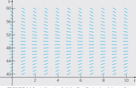
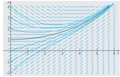
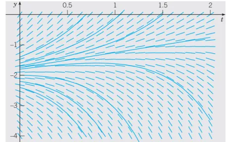
Some Basic Mathematical Models; Direction Fields 5 Direction Fields. Direction fields are valuable tools in studying the solutions of
Some Basic Mathematical Models; Direction Fields 9
Solutions of Some Differential Equations
Solutions of Some Differential Equations 11
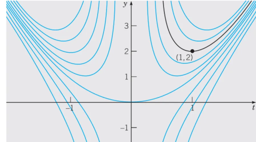
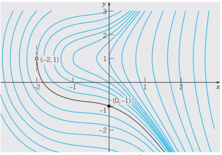
Solutions of Some Differential Equations 13 value of c. Satisfying an initial condition amounts to identifying the integral curve
Classification of Differential Equations 19
Classification of Differential Equations
Classification of Differential Equations 23 If a problem has no solution, we would prefer to know that fact before investing
Classification of Differential Equations 25
Historical Remarks
Historical Remarks 27 the first to publish them, in 1684. Leibniz was very conscious of the power of good
Historical Remarks 29 the ability to solve a great many significant problems within the reach of individual
Linear Equations; Method of Integrating Factors
Linear Equations; Method of Integrating Factors 33 how to find it for a given equation. We will show how this method works first for an
Linear Equations; Method of Integrating Factors 35
Separable Equations
Separable Equations 43 Such an equation is said to be separable, because if it is written in the differential
Separable Equations 45 forms an initial value problem. To solve this initial value problem, we must determine
Separable Equations 47
Separable Equations 49
Modeling with First Order Equations 51
Modeling with First Order Equations
Differences Between Linear and Nonlinear Equations
Differences Between Linear and Nonlinear Equations 69 questions about differential equations and to explore in more detail some important
Differences Between Linear and Nonlinear Equations 71 the proof of Theorem .2 is much more difficult. It is discussed to some extent in
Differences Between Linear and Nonlinear Equations 73
Differences Between Linear and Nonlinear Equations 75 involving t and y that is satisfied by the solution y = φ(t ). Even this can be done
Differences Between Linear and Nonlinear Equations 77
Autonomous Equations and Population Dynamics
Autonomous Equations and Population Dynamics 79 solving the equation. Of fundamental importance in this effort are the concepts
Autonomous Equations and Population Dynamics 81
Exact Equations and Integrating Factors 95
Exact Equations and Integrating Factors
Exact Equations and Integrating Factors 97 The proof of this theorem has two parts. First, we show that if there is a function
Numerical Approximations: Euler’s Method
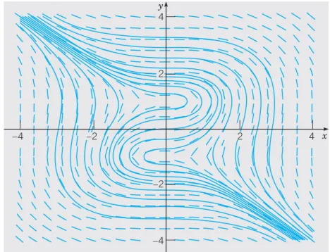
Numerical Approximations: Euler’s Method 103 From the direction field you can visualize the behavior of solutions on the rectangle
Numerical Approximations: Euler’s Method 107 a computer program that will carry out the calculations required to produce results
Numerical Approximations: Euler’s Method 109 To understand better what is happening in these examples, let us look again at
Numerical Approximations: Euler’s Method 111
The Existence and Uniqueness Theorem
The Existence and Uniqueness Theorem 113 but usually does not provide a practical means of finding it. The heart of this method
The Existence and Uniqueness Theorem 115
First Order Difference Equations
First Order Difference Equations 123
Homogeneous Equations with Constant Coefficients
Homogeneous Equations with Constant Coefficients 139 equation (4), or at least to express the solution in terms of an integral. Thus the
Homogeneous Equations with Constant Coefficients 143
Solutions of Linear Homogeneous Equations; the Wronskian 145
Solutions of Linear Homogeneous Equations; the Wronskian

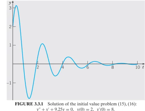
Then solving the initial value problem gives the balanceS(t) in the account at each instant. In other words, the theorem asserts the existence and uniqueness of the solution to the initial value problem (1), (2). With the values ofc1andc2 given by Eq. 23), expression (17) is the solution of the initial value problem.

FIGURE 1.1.2 A direction field for Eq. (5): dv/dt = 9.8 − (v/5).

Existence and Uniqueness Theorem) Consider the initial value problem

Second-order linear equations The operator L is often written as L=D2+pD+q, where D is the derivative operator. Since it is common to use the symbolism to denote φ(t), we will usually write this equation in the form. 2) we associate a set of initial conditions. We would like to know whether the initial value problem (2), (3) always has a solution, and whether there can be more than one solution.

We would also like to know if anything can be said about the shape and structure of solutions that might be useful in finding solutions to specific problems. The fundamental theoretical result for initial value problems for second-order linear equations is stated in Theorem 3.2.1, which is analogous to Theorem 2.4.1 for first-order linear equations. The result applies equally well to non-homogeneous equations, so the theorem is stated in that form.

Nevertheless, theorem 3.2.1 states that this solution is indeed the only solution of the initial value problem (5). For most problems of the form (4) it is not possible to write down a useful expression for the solution. Therefore, all parts of the statement must be proved by general methods that do not involve such an expression. The proof of Theorem 3.2.1 is quite difficult, and we do not discuss it here.2 However, we will accept Theorem 3.2. .1 as true and use it where necessary.

Therefore, the longest open interval containing the initial point t=1, in which all coefficients are continuous, is 0

Principle of Superposition)

Solutions of Linear Homogeneous Equations; the Wronskian 149 The determinant W is called theWronskian 3 determinant,or simply the Wronskian,

Now suppose that y1 and dy2 are two solutions of the equation. Then, as in the examples in Section 3.1, we can generate multiple solutions by forming linear combinations of y1andy2. Therefore, regardless of the values of c1 and c2,yas given by Eq. 7) the differential equation (2) suffices and the proof of Theorem 3.2.2 is complete. The next question is whether all the solutions of Eq. 7) whether there may be other solutions of a different form.

We begin to answer this question by examining whether the constantssc1enc2in Eq. 7) can be chosen such that the initial conditions (3) are met. Sometimes we use the more elaborate notation W(y1,y2)(t0) to calculate the expression on the right-hand side of Eq. 9), highlighting that the Wronskian depends on the function y1andy2, and that it is evaluated at point t0. Then the family of solutions. with arbitrary coefficients sc1 and c2, each solution of Eq. 2) if and only if there is a point 0 at which the Wronskian of y1andy2 is not zero.

Finally, since φ is an arbitrary solution to Eq. 2), it follows that every solution of this equation is included in this family. Choose a pair of such values and choose the solution φ(t) of the equation. 2), which satisfies the initial condition (3). Therefore, it is natural (and we have already done this in the previous section) to call the expression. with arbitrary constant coefficients, the general solution of Eq.

The solutions y1 and y2 are said to form the fundamental set of solutions of the equation. 2) if and only if their Wronskian is nonzero. We can repeat the result of Theorem 3.2.4 in a slightly different language: in order to find a general solution and thus all solutions of an equation of the form (2), we need to find only two solutions of the given equation whose Wronskian is not equal to zero. However, at this stage we can verify by direct substitution that y1indy2 are solutions of the differential equation.

We have used k1andk2 for arbitrary constants in Eq. 20) because they are not the same as the constants c1 andc2 in Eq. Ify=u(t)+iv(t) is a complex-valued solution of Eq. 2), then its real part u and its imaginary part also change the solutions of this equation. Now let us further consider the Wronskian properties of two solutions of a second-order homogeneous linear differential equation.

Abel’s Theorem) 4

Complex Roots of the Characteristic Equation
Complex Roots of the Characteristic Equation 159 What does it mean to raise the number e to a complex power? The answer is provided
Complex Roots of the Characteristic Equation 161
Repeated Roots; Reduction of Order 167
Repeated Roots; Reduction of Order
Repeated Roots; Reduction of Order 169 The procedure used in Example 1 can be extended to a general equation whose
Nonhomogeneous Equations; Method of Undetermined Coefficients 175
Nonhomogeneous Equations; Method of Undetermined Coefficients
Nonhomogeneous Equations; Method of Undetermined Coefficients 177 In somewhat different words, Theorem .2 states that to solve the nonhomoge-

The discussion in this section can be summarized as follows: find the general solution of the differential equation. PROBLEMS In each of Problems 1 through 6, find the Wronskian of the given pair of functions. Show that ify=φ(t) is a solution of the differential equation′′+p(t)y′+q(t)y=g(t), kug(t) is not always zero, thenny=cφ(t ), where any constant other than 1 is not a solution.

In each of problems 24 to 27, check whether the functions y1 and dy2 are solutions of the given differential equation. In each of Problems 29 through 32, find the Wronskian of the two solutions of the given differential equation without solving the equation. In each of Problems 47 through 49, use the result of Problem 46 to find the adjoint of the given differential equation.

For the second-order linear equation P(x)y′′+Q(x)y′+R(x)y=0, show that the adjoint of the adjoint equation is the original equation. The functions y1(t)indy2(t) given by the equations 5) and with the meaning expressed by the equation. 1), when the roots of the characteristic equation (2) are complex numbers λ±iµ. Consequently, if the roots of the characteristic equation are complex numbersλ±iµ, zµ̸=0, then the general solution of the equation is

In this problem, we determine the conditions onpandq that allow Eq. i) convert into an equation with constant coefficients by changing the independent variable. If r1 and r2 are real but not equal, then the general solution of the differential equation is (1). 24) If r1andr2 are complex conjugatesλ±iµ, then there is a general solution. Show that the roots of the characteristic equation are r1=r2=−a, so that one solution of the equation is −at. 23) of Section 3.2] to show that the Wronskian of any two solutions of the given equation is the same.

In each of Problems 23 through 30, use the order reduction method to find a second solution of the given differential equation. In each of Problems 33 through 36, use the method of Problem 32 to find a second independent solution of the given equation. If this is successful, we have found a solution of the differential equation (1) and we can use it for the specific solution Y(t).