貨幣政策中之信用管道：以台灣為例 - 政大學術集成

全文

(1)國立政治大學經濟學系碩士班論文. 政治大. The Credit Channel立 of Monetary Policy: Evidence from Taiwan. ‧ 國. 學. 貨幣政策中之信用管道：以台灣為例. ‧. n. er. io. sit. y. Nat. al. Ch. engchi. i n U. v. 指導教授：朱美麗博士研究生：王安中. 中華民國九十九年七月.

(2) 致謝詞經過了漫長的過程，還曾經還懷疑我走不走的完這條路。一路走來得到無數的支持，我終於畢業了！最先要感謝前政大經濟系的高安邦老師以及政大財政系的黃智聰老師。在他們的引導之下我決定了經濟研究所這條路。當然，有了彭彥熹學長給我強力惡補一下才能正式走上這條路。另外也要感謝陳鎮洲老師、莊奕琦老師和毛維凌老師，在我決定走經研所這條路後願意給我機會複習大學時所讀的，以及讓我這個美國人盡早適應台灣的上課模式（一次上三小時課真的需要極好的集中能力與耐力！）。經過了兩年（又八個多月）的過程，老師們除了給我大大小小的意見之外，也讓我多學了很多新的經濟理論。首先感謝吳中書老師以及翁永和老師，在口試的時候給了我許許多多寶貴的意見。謝謝簡義哲學長，在寫論文的過程中也給了我許多建議。另外還有給予計量方面指導的林馨怡老師以及徐士勛老師，得以讓我用最好的計量方法得到最好的結果。另外，黃仁德老師、黃俞寧老師、林祖嘉老師、廖郁萍老師、李慧琳老師、李文福老師以及洪福聲老師在課堂上所教的也讓我發現我所知道的經濟學是一個非常有趣，也非常寬廣的領域。在這邊也要感謝劉小蘭老師以及王大立老師，在寫論文的過程中用他們的專業來教導我最好的寫法以及包裝方法。最後要感謝我家人，尤其爸爸和媽媽，在這段時間給我支持與鼓勵。也要感謝妹妹，在我已經沒動力的時候讓我有機會回美國看一場我最喜歡的美國職棒大聯盟球賽和美國職業冰球的季後賽，讓我加油繼續下去。. 立. 政治大. ‧. ‧ 國. 學. n. er. io. sit. y. Nat. al. Ch. engchi. i n U. v.

(3) Abstract The credit market is an important subject in today’s macroeconomic world. Prior to the introduction of the credit market, traditional models only included the goods market and money market to form the IS-LM model. Under this IS-LM model, a change in money supply would have a known effect, such as a monetary expansion policy will result in a drop in the bond rate because the IS curve will remain constant. However, many previous studies did not show this effect, but instead the opposite; those that did show this effect, the magnitude of the shift was different than a traditional IS-LM model. Once the credit market is introduced into the IS-LM model, both the goods market (IS curve) and the money market (LM curve) will shift, resulting in an undetermined change in bond rate, and will also introduce the loan rate, which also shows an undetermined change. Under this model, when a monetary expansionary policy is in effect, it is possible that the bond rate could decrease, increase, or remain constant. This thesis will determine how the credit channel operates in Taiwan, using quarterly data from 1992Q1 to 2009Q4. The final result shows that under this new model, the credit channel in Taiwan does not necessarily follow the previously-known theory.. 立. 政治大. ‧. ‧ 國. 學. Key words: Credit channel, monetary policy, interest rates. n. er. io. sit. y. Nat. al. Ch. engchi. i n U. v.

(4) Table of Contents Chapter 1: Introduction and Literature Review…..………………………………….……………….. 1 Chapter 2: The Theoretical Model…………………………………………………………………………… 4 2.1: Loan Market.…………………………………………..………………………………………………… 4 2.2: Money Market...……………………………………………………………………………………….. 5 2.3: Good Market…………………………………………………………………………………………….. 5 2.4: The Effect of a Change in Bank Reserves…………………………………………………… 5 2.5: Graphical Representation…………………………………………………………………………. 7 2.5.1: LM Curve……………………………...……………………………………………………….. 7 2.5.2: CC Curve………………………………………………………………………………………… 8 2.5.3: The Effect of Reserve Money Change on Bond Rate…..…………………. 10 2.5.4: The Effect of Reserve Money Change on Loan Rate.……………………… 13 2.6: Summary………………………………………………………………………………………………… 16. 立. 政治大. ‧. ‧ 國. 學. Chapter 3: Methodology and Test Results……………………………………………..………………. 17 3.1: Methodology and Data…………………………………………………………..………………. 17 3.2: Test Results…………………………………………………………………………..………………… 20 3.2.1: VAR Setup………………………………………………………………..………………….. 20 3.2.2: Effect on MONEYRATE…………………………………………………………………. 20 3.2.3: Effect on GDPSA…………………………………………………………………………… 20 3.2.4: Effect on INTEREST……………………………………………………………………….. 21 3.2.5: Considering 1997 Asian Financial Crisis and 2008 Global Financial Crisis………………………………………………………………………………………………………. 21 3.3: Summary…………………………………………………………………………..……………………. 21. n. er. io. sit. y. Nat. al. Ch. engchi. i n U. v. Chapter 4: Conclusion……………………………………………………………..……………………………. 24 References…………………………………………………………………………..………………………………… 25 Data Sources………..……………………………………………………………………………………………….. 26 Appendix…………………………………………………………………….…………………………………………. 28.

(5) Chapter 1: Introduction and Literature Review The credit market is an important subject in today’s macroeconomic world. Before the credit market was looked at, a traditional model containing the goods market and money market were put together to form the IS-LM model. Under this IS-LM model, a change in monetary policy would only shift the LM curve while the IS curve remained constant. In such case, one can see how output and interest rates would change in response to the monetary policy applied. However, Bernanke and Blinder (1988) introduced the credit channel by way of the credit and commodity (CC) curve to the IS-LM model. The assumption under Bernanke and Blinder (1988) is that under an IS-LM model, bonds and loans are not perfect substitutes, as previous studies assumed that only money and bonds existed or that loans and bonds are perfect substitutes. Once this new assumption was taken into place, the traditional IS-LM model was modified with money, bonds and loans being unique assets, which is shown as the CC curve replacing the IS curve in the traditional IS-LM model and becoming a CC-LM model. When a monetary policy change is implemented, this case would not only shift the LM curve, but as a result will also shift the CC curve. For example, under an IS-LM model, a monetary expansion policy will lead to the LM curve shifting outwards, while the IS curve stays put. This would result in an increase in total output and a decrease in interest rates. When the CC curve is introduced into the model, under the same expansionary policy, the LM curve will shift outward, but the CC curve may also shift due to the policy. It is possible that the CC curve would shift inward, outward, or even stay constant, resulting in interest rates decreasing, remaining constant, or increasing. Under this scenario, total output would increase as a result of the LM curve’s shift, but because of the CC curve’s possible shifts (or no shift), the change in the interest rate is not known. Many future literatures have looked into this effect and test for the resulting changes between interest rates and output. Bernanke and Gertler (1995) used US data to test this new credit channel to see whether theory matches reality. Bernanke and Gertler look at how output levels would change when a monetary tightening policy is implemented, and all the changes that occur along the way which leads to the resulting output level change. Bernanke and Gertler use a vector autoregression (VAR) model to determine such effects with monthly data. With this model, they try to emphasize four different facts about the economy when such a monetary tightening policy is implemented, one of which states that while an unanticipated tightening will have a transitory effect on interest rates, it will have a sustained effect on the decline in GDP. When a test is performed with log real GDP, it shows a 4-month lag from when the tightening policy. 立. 政治大. ‧. ‧ 國. 學. n. er. io. sit. y. Nat. al. Ch. engchi. i n U. v. 1.

(6) is implemented to when GDP starts its decline. Also, the results show that interest rates will rise initially, before beginning to decline. As theory shows that interest rates decline only when there is a monetary expansion policy, this case will only occur under Bernanke and Blinder’s 1988 model when the CC curve shifts in a way that allow interest rates to fall below the initial level. In addition to Bernanke and Gertler, Bernanke and Blinder (1992) used their 1988 model as a starting point to determine which economic variable would be the best predictor to the future trend of the economy. Similar to Sims (1980) and Litterman and Weiss (1985), a VAR model is constructed, showing that the Federal Funds rate has a higher level of predicting power when compared to money supply, which contrast previous theories. To prove this, Bernanke and Blinder, using monthly data from 1959:7 to 1989:12, take MacCallum’s (1983) suggestion to Sims by using money supply M1 and M2, different policy variables (Federal Funds rate, Treasury bill rate, and Treasury bond rate), and different measures of forecasting power to show the better predicting ability. The results show that the Federal Funds rate outperforms every other interest rate, and that the money supply’s predicting power is limited, with M1 showing no predicting power at all. While Bernanke and Blinder’s results show Federal Funds rate as the best economic predictor, however, because there is no perfect substitute for the Federal Funds rate in Taiwan, the closest alternative for Taiwan would be the overnight rate or the discount rate. By way of the credit channel, Hulsewig, Mayer and Wollmershauser (2006) look at the bank loan supply and monetary policy transmission in Germany. GDP, CPI, short term rate, and loan rate data from 1991Q1 to 2003Q2 were collected and used to determine how certain economic factors would change when a monetary policy shock was implemented by using a VAR model. Hulsewig et al find that when a shock is implemented, short term rate, loan interest rate, price levels, output levels, and bank loans will decline, similar to De Bondt (2000), and Holtemoller (2003). The output level in particular would drop for about four quarters before gradually returning to the original level, which corresponds to the evolution of the output gap. Most literature found that a monetary tightening policy would lead to a drop in interest rates. This drop, in turn, would lead to a decrease in overall output levels. However, previous theories, particularly those involving the IS-LM model, showed that a monetary tightening policy would lead to a rise in interest rates. The results from the literature show that should happen in theory and what does happen in reality are different. As opposed to theory, this situation will occur only in a model that includes the credit channel with dynamics that allow for the interest rate to drop, which is only possible with a CC-LM model. Also, Bernanke and Blinder (1992) used various economic activities to determine the best economic predictor and came up. 立. 政治大. ‧. ‧ 國. 學. n. er. io. sit. y. Nat. al. Ch. engchi. i n U. v. 2.

(7) with the conclusion of the Federal Funds rate being the best, but did not make any references as to whether the Federal Funds rate is the best predictor to overall economic output. However, the lack of using total GDP as an economic factor was covered by Bernanke and Gertler (1995). While Hulsewig, et al (2005) did include total output in their model, they used it to determine the response of bank loans, which is opposite of others that use changes in interest rates or loan demand to determine the changes in total output. While there have been many previous literatures and studies on this topic, very few have either come from Taiwan, or look at how the credit channel operates in Taiwan. One of the few that did so was done by Wu and Chen 1 (2004). Wu and Chen looked at the lending patterns by individual households and corporations, and determined which had a bigger impact on total output. They conclude that under the same monetary policy, individual lending has a significant positive impact on total output, while corporate lending did not show a significant impact. Also, Ho 2 (2001) determines the relationship between the overnight money rate and deposit and loan rates by looking at the rate of the resulting changes to the deposit and loan rate when there is a change in the overnight rate. Using Klein’s (1971) assumption of a loan demand curve being negatively sloped and a loan supply curve being positively sloped, and the maximum profit conditions stated by Hannan and Berger (1991) and Cottarelli and Kourelis (1994), the conditions of how often a bank adjusts loan rates. However, when this case was applied to Taiwan, the results were inconclusive as this change was not shown when the overnight rate was present. However, applying Taiwan’s case with the Error-Correction Model, Ho’s results show that when the overnight money rate changes, the deposit and loan rates will lag behind, but will change, and in the opposite direction of the overnight money rate. This thesis will use data from Taiwan to see the relationship between money supply, interest rates, and output and check whether these movements match theory, or what has already been founded in previous literatures. In contrast to Wu and Chen, this thesis combines both household loans and corporate loans into one, and determines the impact on total output in Taiwan. In addition, this thesis will also test for the role that monetary policy plays when it comes to changes in the output level and also check whether it matches theory or previous literatures.. 立. 政治大. ‧. ‧ 國. 學. n. er. io. sit. y. Nat. al. 1 2. Ch. engchi. i n U. v. 吳中書，陳立修何棟欽 3.

(8) Chapter 2: The Theoretical Model The theoretical model used in this thesis is based on Bernanke and Blinder (1988), which will be used to determine the effects of output and the interest rate from a change in monetary policy. In theory, under a traditional IS-LM model, a change in monetary policy will have a definitive change in both output and interest rates based on the policy implemented, but in the model described by Bernanke and Blinder (1988), the output change is definitive but the bond rate change is unknown. Previously, as shown in Bernanke and Blinder (1988), only the plus-minus relationships are shown between variables without looking into the interaction between variables. The model shown here, using the framework of Bernanke and Blinder’s model, will solve the exact interaction between each variable and how the resulting plus-minus relationship is determined. From Bernanke and Blinder (1988), there are three different markets: the loan market, the goods market, and the money market. This paper studies the effects of a change in bank reserves on the loan rate, bond rate, and output.. 政治大. 立. ‧ 國. 學. 2.1. Loan Market. ‧. Loan demand is defined as:. y. Nat. sit. n. al. er. io. L(ρ, i, y) …………………………………………………………….…………………………………………….. (2.1a) (Lρ < 0, Li > 0, Ly > 0). Ch. i n U. v. In equation (2.1a), ρ is the interest rate on loans, i is the interest rate on bonds, and y is income. Total loan demand is a function of the interest rate on loans, interest rate on bonds, and total income. The loan rate is inversely related to loan demand, meaning a rise in the loan rate will decrease loan demand. Both bond rate and income are positively related to loan demand, meaning an increase in either will result in an increase in loan demand.. engchi. Loan supply is defined as: λ(ρ, i)D(1 − τ) ……………………………………………………………………………………………….. (2.1b) (λρ > 0, λi < 0) In equation (2.1b), τ is the required reserve rate, and D is total deposits. Loan supply is defined as the multiplication of λ, D, and (1 - τ). λ is the credit supply. 4.

(9) function, and is a function of the loan rate and bond rate. D is in function form, and will be discussed more in the next section. While λ and the loan rate are positively related, λ and the bond rate are inversely related, meaning that a rise in the loan rate will increase credit supply, while a rise in the bond rate will decrease credit supply. In order for the loan market to reach equilibrium, loan supply must equal loan demand. This allows us to obtain the loan market equation: L(ρ, i, y) = λ(ρ, i)D(1 − τ) ……………………………………………………..……………………….. (2.1) 2.2. Money Market. The money market equilibrium is defined as total deposits equaling total reserves multiplied by the money multiplier, shown as:. 政治大 D(i, y) = m(i)R ……………………………………………………………………..………………………… (2.2) 立 (D < 0, D > 0, m > 0) i. ‧ 國. y. 學. i. ‧. In equation (2.2), R represents bank reserves, and m represents the money multiplier. Total deposit is a function of the bond rate and income, where the bond rate and total deposit are inversely related, while income and total deposits are positively related. The money multiplier is a function of the bond rate, and the money multiplier is positively related to the bond rate.. n. al. er. io. sit. y. Nat. 2.3. Goods Market. Ch. The goods market is defined as:. engchi. i n U. v. y = Y(i, ρ) …………………………………………………………………………………………………………. (2.3) (Yi < 0, Yρ < 0) Total output is represented as aggregate demand, which is a function of both the loan rate and bond rate. Both interest rates are inversely related to aggregate demand. 2.4. The Effect of a Change in Bank Reserves After differentiating equations (2.1), (2.2), and (2.3) 3, we then organize the 3. See Appendix for step-by-step process. 5.

(10) resulting differentiated equations into matrix form: �Lρ − m(i)R(1 − τ)λρ � [Li − λ(ρ, i)mi (1 − τ)R − m(i)R(1 − τ)λi ] (Di − mi R) � 0 −Yρ −Yi. dρ λ(ρ, i)m(i)(1 − τ) � di � = � � [dR] m(i) dy 0. Ly Dy � ∗ 1. Next, we solve the determinant for the 3*3 matrix, which we label as K: |K| = ��Lρ − m(i)R(1 − τ)λρ � ∗ (Di − mi R) ∗ 1� + �[Li − λ(ρ, i)mi (1 − τ)R − m(i)R(1 − τ)λi ] ∗ Dy ∗ �−Yρ �� − �Ly ∗ (Di − mi R) ∗ �−Yρ �� − ��Lρ − m(i)R(1 − τ)λρ � ∗ (−Yi ) ∗ Dy � ≶ 0 ………………………………………………………………………………………….………………………………. (2.4). 政治大. 立. ‧ 國. 學. ‧. The sign of the determinant is undetermined, but using the assumption 4 mi = 0, the determinant becomes:. n. al. er. io. sit. y. Nat. |K| = ��Lρ − m(i)R(1 − τ)λρ � ∗ (Di ) ∗ 1� + �[Li − m(i)R(1 − τ)λi ] ∗ Dy ∗ �−Yρ �� − �Ly ∗ (Di ) ∗ �−Yρ �� − ��Lρ − m(i)R(1 − τ)λρ � ∗ (−Yi ) ∗ Dy � > 0 ………………………………………………………………………….………………………………………………. (2.5). Ch. i n U. v. This provides us with a positive determinant, and we can solve how the total reserves would change when the loan rate, bond rate, and income changes. dρ First, we solve for �dR, which represents the relationship of how total. engchi. reserves would change when the loan rate changes, which equals: dρ. dR. =. |A|. |K|. ≶ 0 ……………………………………………………………………………….……………………… (2.6). |A| = {λ(ρ, i)m(i)(1 − τ) ∗ (Di − mi R) ∗ 1} + {Ly ∗ (−Yi ) ∗ m(i)}. 4. − {[Li − λ(ρ, i)mi (1 − τ)R − m(i)R(1 − τ)λi ] ∗ m(i) ∗ 1} − {λ(ρ, i)m(i)(1 − τ) ∗ (−Yi ) ∗ Dy } ≶ 0. As long as the money multiplier isn’t too large,. dm di. = mi → 0. 6.

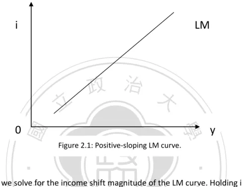
(11) This relationship is undetermined. Therefore, we must discuss further to know the exact effect. Next, we solve for di�dR, which represents the relationship of how total. reserves would change when the bond rate changes, which equals: di. dR. =. |B|. |K|. ≶ 0 ………………………………...………………………………………………………..…………. (2.7). |B| = ��Lρ − m(i)R(1 − τ)λρ � ∗ m(i) ∗ 1� + �λ(ρ, i)m(i)(1 − τ) ∗ Dy ∗ �−Yρ �� − �Ly ∗ m(i) ∗ �−Yρ �� ≶ 0. 政治大. ‧ 國. 立. 學. The relationship is undetermined. Therefore, we must discuss further to know the exact effect. dy Finally, we solve for �dR, which represents the relationship of how total reserves would affect income, which equals:. > 0 ………………………………………….…………………………………………………………… (2.8). y. sit. |C|. |K|. ‧. =. Nat. dy. dR. n. al. er. io. |C| = {[Li − λ(ρ, i)mi (1 − τ)R − m(i)R(1 − τ)λi ] ∗ m(i) ∗ �−Yρ � − �λ(ρ, i)m(i)(1 − τ) ∗ (Di − mi R) ∗ �−Yρ ��. Ch. i n U. v. − {�Lρ − m(i)R(1 − τ)λρ � ∗ �−Yρ � ∗ m(i)} > 0. engchi. The result shows that the relationship between bank reserves and income is positively related, indicating that an increase in income would result in an increase in reserves. 2.5. Graphical Representation 2.5.1. LM Curve The LM curve is defined as the money market shown in equation (2.2). We solve for the slope of the LM curve, which is defined as di�dy |LM : 7.

(12) di | dy LM. =. Dy. > 0 …………………………………………………………….……………………………. (2.9). mi R−Di. This shows that the LM curve has a positive slope, which is illustrated in Figure 2.1.. i. LM. 立. 政治大. ‧ 國. 學. 0. y. Figure 2.1: Positive-sloping LM curve.. ‧. n. al. er. io. sit. y. Nat. Next, we solve for the income shift magnitude of the LM curve. Holding i constant, we can solve for the income shift magnitude when the reserve money dy increases, which is defined as �dR |LM . The resulting shift magnitude equals: dy. dR. |LM =. m(i) Dy. Ch. engchi. i n U. v. > 0 ..………………………………….…………………………………..………………….. (2.10). 2.5.2. CC Curve The CC curve is very similar to the IS curve in the traditional IS-LM model. The main difference is that aspects of the loan market does not affect movements of the IS curve, while the CC curve is affected by changes in the loan market, particularly the loan rate. The CC curve representing the combination of the bond rate and output level that allows both the goods market and the loan market to be at equilibrium. As stated by Bernanke and Blinder (1988), given that the loan rate ρ can be written as a function of i, y, R, we can write ρ as: 8.

(13) ρ = ρ(i, y, R) …...........……………………………………………………………………………………… (2.11) Differentiating ρ and using the differentiated equation (2.11), we can get:. ρi = −. [Li −λ(ρ,i)mi (1−τ)R−m(i)R(1−τ)λi ]. ρy = − ρR =. �Lρ −m(i)R(1−τ)λρ � Ly. �Lρ −m(i)R(1−τ)λρ �. λ(ρ,i)m(i)(1−τ). �Lρ −m(i)R(1−τ)λρ �. ≶ 0…………………………….…………………………. (2.12a). > 0………………………………………………….……………………….. (2.12b). < 0…………………………………………………….………………………… (2.12c). The sign of ρi is undetermined. However, by using the assumption mi = 0 as shown in footnote (2), we get:. ‧ 國. �Lρ −m(i)R(1−τ)λρ �. 立. > 0 ………………………………………………..………………………… (2.12d). 學. ρi = −. [Li − m(i)R(1−τ)λi ]. 政治大. ‧. Equation (2.12b) shows that loan rate and income are positively related. Equation (2.12c) shows that the loan rate and reserves are inversely related. Equation (2.12d) shows that the loan rate and bond rate are positively related. Substituting equation (2.11) into equation (2.3), we can get the CC curve equation:. n. er. io. sit. y. Nat. al. Ch. i n U. v. y = Y(i, ρ(i, y, R)) …………..................................................................................... (2.13). engchi. We solve for the slope of the CC curve, which is defined as di�dy |CC :. di. dy. |CC =. 1−Yρ ρy. Yi +Yρ ρi. < 0 ……………………………………..………………………………….……………… (2.14). This shows that the CC curve has a negative slope, which is illustrated in Figure 2.2.. 9.

(14) i. CC 0. y. Figure 2.2: Negative-sloping CC curve. Next, we solve for the income shift magnitude of the CC curve. Holding i constant, we can solve for the income shift in the magnitude of the CC curve when dy total reserves increase, which is defined as �dR |CC . The magnitude of the income. 立. shift on the CC curve equals:. ‧ 國. Yρ ρR. 1−Yρ ρy. > 0 ..………………………………………………..…………………..…………….. (2.15) 5. 2.5.3. The Effect of Reserve Money Change on Bond Rate. Nat. y. ‧. =. 學. dy | dR CC. 政治大. sit. n. al. er. io. After solving equations (2.10) and (2.15), we can see that both the income shift and the bond rate shift of both CC and LM curves are positively related to changes in bank reserves. Next, using these equations, we solve for Yρ , which represents how. Ch. i n U. v. income changes when the loan rate changes. Setting both equations equaled to each other, we get: Yρ ρR. 1−Yρ ρy. =. m(i) Dy. engchi. …………………………………………………………………….……..………………... (2.16). Using equation (16), we can solve for Yρ , which equals: Yρ = 5. 6. m(i). Dy ρR +m(i)ρy. ………………………………………………………………………………………… (2.17) 6. Y �. λ(ρ,i)m(i)(1−τ). ρ �L −m(i)R(1−τ)λ � Yρ ρR ρ ρ dy� | = = CC Ly dR 1−Yρ ρy 1−�Y ��−. Yρ =. m(i). Dy ρR +m(i)ρy. =. ρ. Dy. �. �Lρ −m(i)R(1−τ)λρ �. m(i). �. Ly λ(ρ,i)m(i)(1−τ) +m(i)�− � �Lρ −m(i)R(1−τ)λρ � �Lρ −m(i)R(1−τ)λρ �. 10.

(15) Reorganizing the complex version of equation (2.17) as described in footnote (3), we can obtain: −Yρ �Dy λ(ρ, i)m(i)(1 − τ) − m(i)Ly � + m(i)�Lρ − m(i)R(1 − τ)λρ � = 0 … (2.18). The left hand side of equation (2.18) is the same as |B| in equation (2.7). Therefore, in the condition set in equation (2.18), the shift magnitude of CC and LM are equal. After solving for Yρ , there are three possible results: 1. If Yρ <. m(i). Dy ρR +m(i)ρy. 政治大. , corresponding back to equation (2.18), this would set |B| to. 立. be greater than zero. Substituting this condition back into equation (2.7),. ‧ 國. 學. would be positive, resulting in di�dR being positive. This shows that the. |B| �|K|. sit. , corresponding back to equation (2.18), this would set |B| to. io. Dy ρR +m(i)ρy. al. er. m(i). y. Nat. 2. If Yρ >. ‧. magnitude of the CC shift is greater than the magnitude of the LM shift, resulting in the bond rate increasing. Figure 2.3 illustrates this result.. v ni. n. be less than zero. Substituting this condition back into equation (2.7),. Ch. would be negative, resulting in. U i e h n c g di. |B| �|K|. �dR being negative. This shows that the. magnitude of the CC shift is less than the magnitude of the LM shift, resulting in the bond rate decreasing. Figure 2.4 illustrates this result. 3. If Yρ =. m(i). Dy ρR +m(i)ρy. , corresponding back to equation (2.18), this would set |B|. equaled to zero. Substituting this condition back into equation (2.7),. |B| �|K|is. equaled to zero, resulting in di�dR equaling zero. This shows that the magnitude of the CC shift equals the magnitude of the LM shift. Corresponding back to. 11.

(16) equation (2.7) di�dR must equal zero, resulting in the bond rate remaining the same. Figure 2.5 illustrates this result.. i. i. LM. LM. LM LM’ CC’. CC. 政治大 y Figure 2.4: LM shift > CC shift,. 立 resulting in the bond rate. Figure 2.3: CC shift > LM shift,. resulting in the bond rate. ‧ 國. decreasing.. i. ‧. LM. Nat. LM’. LM. sit. n. er. io. al. Ch. engchi. CC’. i n U. v. CC. CC Figure 2.5: CC shift = LM shift, resulting in the bond rate remaining the same.. LM’. y. i. y. 學. increasing.. CC’. CC. y. Figure 2.6: Special case where Yρ =. y. 0. LM shifts (magnitude unknown),. but CC curve remains constant, as the bond rate decreases.. A special case of this model occurs when Yρ = 0. In this scenario, any monetary policy shift will keep the CC curve constant and shift only the LM curve. Also, as Yρ is negative in theory, setting Yρ = 0 would result in Yρ >. m(i). Dy ρR +m(i)ρy. , which is the. 12.

(17) same condition as described in the 2nd possible result. Figure 2.6 illustrates this special case.. 2.5.4. The Effect of Reserve Money Change on Loan Rate After differentiating equations (2.2) and (2.13), we can solve for the interest rate shift magnitude for both LM and CC curves, which are defined as di�dR |LM and di� | , respectively. dR CC. =. Yρ ρR. −Yi +Yρ ρi m(i). 政治大. …………………………….…………………………………..…………………………… (2.19). 立. ……………………………………………………………………….………………………... (2.20). Di −mi R. 學. di | dR CC. =. ‧ 國. di | dR LM. Yi m(i). < 0…………………………………….…………………………………….……. (2.21). sit. er. io. ρR Di −ρR mi R+ρi. y. Nat. Yρ = −. ‧. Setting both equations (2.19) and (2.20) equal to each other and reorganizing both, we can solve for Yρ , which is equal to:. Using equation (2.21), we can come up with three possible results:. n. al. 1. If Yρ < −. Yi m(i). ρR Di −ρR mi R+ρi. Ch. engchi. i n U. v. , then the magnitude of the CC curve shift is greater than. the LM curve shift. This will result in the loan rate increasing, making. equation (2.6). 2. If Yρ > −. Yi m(i). ρR Di −ρR mi R+ρi. > 0 in. , then the magnitude of the LM curve shift is greater than. the CC curve shift. This will result in the loan rate decreasing, making. equation (2.6).. dρ. dR. dρ. dR. < 0 in. 13.

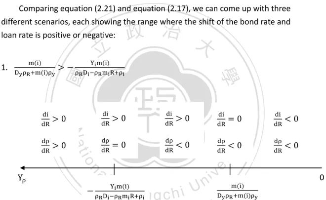
(18) 3. If Yρ = −. Yi m(i). ρR Di −ρR mi R+ρi. , then the magnitude of the LM curve shift and the CC. curve shift are equal. This will result in the loan rate remaining constant, dρ. making. dR. = 0 in equation (2.6).. A unique scenario occurs when Yρ = 0. In this scenario, any monetary policy shift will keep the CC curve constant and shift only the LM curve. Setting Yρ = 0 would result in Yρ > − possible result.. Yi m(i). ρR Di −ρR mi R+ρi. , which is the same condition as described in the 2nd. Comparing equation (2.21) and equation (2.17), we can come up with three different scenarios, each showing the range where the shift of the bond rate and loan rate is positive or negative:. Yρ. al. −. dρ. =0. Ch. Yi m(i). dR. <0. engchi. ρR Di −ρR mi R+ρi. di. >0. dR dρ. =0. y. dR. <0. sit. di. >0. dR. er. dρ. dR. n. >0. di. dR. ‧. >0. io. dρ. dR. ρR Di −ρR mi R+ρi. Nat. di. dR. >−. ‧ 國. Dy ρR +m(i)ρy. 立. Yi m(i). 學. 1.. m(i). 政治大. i n U. v. di. dR dρ. dR. <0 <0 0. m(i). Dy ρR +m(i)ρy. Figure 2.7. Graphical representation of the shift in the bond rate and loan rate for different values of Yρ. when. 2. If. m(i). Dy ρR +m(i)ρy. m(i). Dy ρR +m(i)ρy. >−. <−. Yi m(i). ρR Di −ρR mi R+ρi. .. Yi m(i). ρR Di −ρR mi R+ρi. 14.

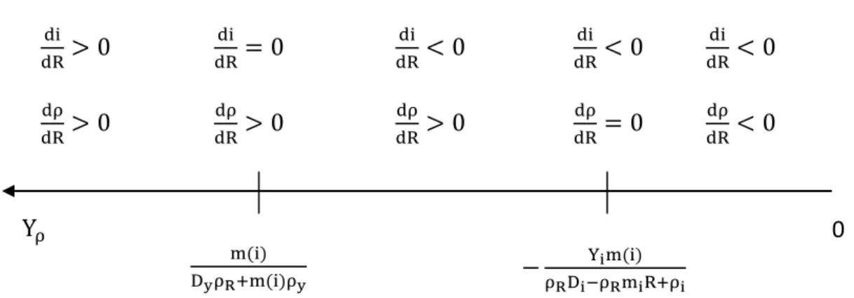
(19) di. dR dρ. dR. di. >0. dR dρ. >0. dR. Yρ. di. =0. dR dρ. >0. dR. di. <0. dR dρ. >0. m(i). dR. −. Dy ρR +m(i)ρy. di. <0. dR dρ. =0. dR. <0 <0 0. Yi m(i). ρR Di −ρR mi R+ρi. Figure 2.8. Graphical representation of the shift in the bond rate and the loan rate for different. m(i). =−. Dy ρR +m(i)ρy. Yi m(i). ρR Di −ρR mi R+ρi. Yi m(i). 治政 , 大. ρR Di −ρR mi R+ρi. 立. di. dρ. >0. dR. Nat. io. Yρ. dR. di. =0. dR dρ. =0. <0. dR. <0 0. y. dρ. dR. >0. ‧. ‧ 國. dR. .. 學. di. <−. m(i). Dy ρR +m(i)ρy. n. al. =−. Yi m(i). sit. 3. If. m(i). Dy ρR +m(i)ρy. ρR Di −ρR mi R+ρi. er. values of Yρ when. i n U. v. Figure 2.9. Graphical representation of the shift in the bond rate and the loan rate for different values of Yρ when. m(i). Ch. Dy ρR +m(i)ρy. =−. e n g c. h i Yi m(i). ρR Di −ρR mi R+ρi. Figures 2.7, 2.8, and 2.9 show the shifts in the loan rate and bond rate during a monetary policy change at different values of Yρ . As seen in Figures 2.7 and 2.8, there are values of Yρ where the bond rate change and the loan rate change are opposite of each other. The change in both the bond rate and the loan rate are in opposite directions, with the value of. m(i). Dy ρR +m(i)ρy. and −. Yi m(i). ρR Di −ρR mi R+ρi. and the value of Yρ deciding. which one increases and which one decreases. In such a case, as the change is opposite of one another, the overall change would be less than if only one type of interest rate were present. 15.

(20) In Figure 2.9, the change in both the bond rate and the loan rate are in the same direction, with the change either positive or negative depending on the value of Yρ . In this case, as the change is in the same direction, the overall change would be greater than if only one type of interest rate were present. 2.6. Summary In theory, a simple IS-LM model will have known effects. For example a monetary expansion policy will shift the LM curve to the right, resulting in total output increasing and bond rate decreasing, and vice versa. However, when a CC curve is in place of the IS curve, a change in the monetary policy will shift the LM curve and the new CC curve as well. As shown in the cases described in Figures 2.3, 2.4, 2.5, and 2.6, the overall income will increase, but the magnitude of the change is different depending on the shift magnitudes of the LM and CC curve. As seen in the graphs, Figure 2.4 shows the greatest increase in income, Figure 2.5 the second-greatest, and Figure 2.3 the least. However, the change in income for Figure 2.6 is undetermined as the change depends solely on the shift magnitude of the LM curve. This needs to be discussed further for the exact change in income and both the bond rate and interest rate to be known. The next section will determine this exact effect using data from Taiwan. This will then describe the situation, from the above results, that applies in Taiwan.. 立. 政治大. ‧. ‧ 國. 學. n. er. io. sit. y. Nat. al. Ch. engchi. i n U. v. 16.

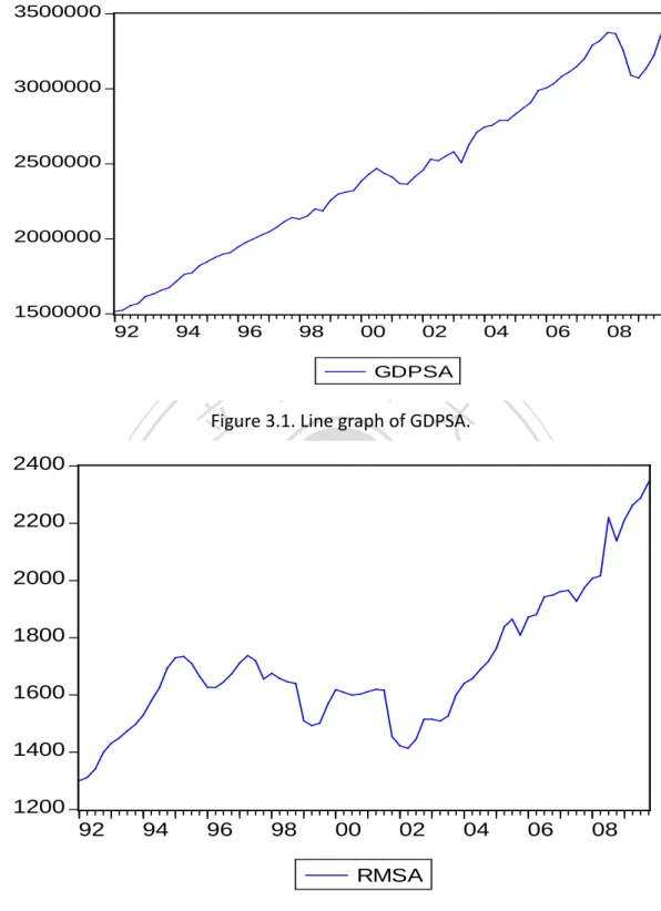
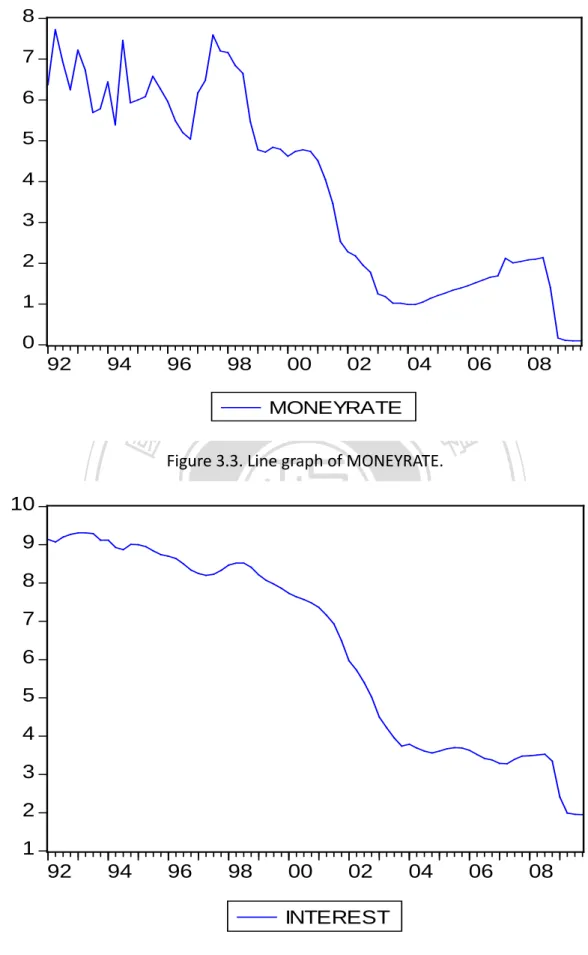
(21) Chapter 3: Methodology and Test Results 3.1 Methodology and Data Using the model described by Bernanke and Blinder (1988), as shown in Chapter 2, a test was performed to see how interest rates would change during a change in monetary policy. The data within the model consists of the real GDP, reserve money supply, loan interest rate (INTEREST), and the overnight money rate 7 (MONEYRATE) from Taiwan between the first quarter of 1992 to the fourth quarter of 2009. The overnight money rate was chosen as a substitute to the bond rate described in Chapter 2 as Taiwan does not have an exact match of the bond rate as seen in the US or Europe. Real GDP, in million NT, is seasonally adjusted (GDPSA). Also, since the unit of reserve money was in million NT, it is seasonally adjusted (RMSA) to be consistent with GDP. Figures 3.1-3.4 show the trend line graph of GDPSA, RMSA, MONEYRATE, and INTEREST respectively. After performing the necessary adjustments of the data, a cointegration test is performed with EViews to determine if there were any cointegrating equations. The final cointegration result showed that there were no cointegrating equations, therefore a vector autoregression (VAR) equation was set up. The VAR setup had GDPSA and MONEYRATE, and INTEREST as endogenous variables, while the exogenous policy variable is RMSA. From this set up, we will be able to see how RMSA will affect all other endogenous variables by looking at the coefficient’s sign and whether the resulting coefficient is statistically significant or not. The RMSA coefficient for MONEYRATE is of particular interest in this thesis, as it will give a clear indication of whether the change is positively related or inversely related. From this result, we are able to determine whether Taiwan’s credit channel follows the theoretical model or is different than in theory.. 立. 政治大. ‧. ‧ 國. 學. n. er. io. sit. y. Nat. al. 7. Ch. engchi. i n U. v. 隔夜拆款利率 17.

(22) 3500000. 3000000. 2500000. 2000000. 1500000 92. 98. 96. 94. 02. 00. 04. 06. 08. 政治大 Figure 3.1. Line graph of GDPSA. 立 GDPSA. 2200 2000. ‧. ‧ 國. 學. 2400. n. al. er. io. 1600. sit. y. Nat. 1800. 1400. Ch. engchi. i n U. v. 1200 92. 94. 96. 98. 00. 02. 04. 06. 08. RMSA. Figure 3.2. Line graph of RMSA.. 18.

(23) 8 7 6 5 4 3 2 1 0 96. 94. 立. Figure 3.3. Line graph of MONEYRATE.. y. sit. io. al. n. 7. er. 8. 6. 08. MONEYRATE. Nat. 9. 06. ‧. 10. 政 00 治02 大04. 98. 學. ‧ 國. 92. Ch. 5. engchi. i n U. v. 4 3 2 1 92. 94. 96. 98. 00. 02. 04. 06. 08. INTEREST Figure 3.4. Line graph of INTEREST.. 19.

(24) 3.2. Test Results 3.2.1. VAR Setup The model involves using RMSA as an exogenous variable. After testing for the best lag length to use and whether there were any cointegrating equations, the conclusion was reached that for this model in particular, 3 lags would be used since the AIC value is the lowest at the 3rd lag level. Since there are no cointegrating equations, a VAR was used for this model. The final VAR equation is equaled to: GDPSAt � INTERESTt � = MONEYRATEt. A211,t−1 C12 G12 �C22 � + �G22 � [RMSA] + �A221,t−1 C32 G32 A231,t−1. t−1. t−1. MONEYRATEt−1. �+ ⋯+. ‧ 國. A213,t−2 e12 GDPSAt−3 A223,t−2 � � INTERESTt−3 � + �e22 �……………………………………. (3.2a) e23 A233,t−2 MONEYRATEt−3. ‧. A212,t−2 A222,t−2 A232,t−2. 2 13,t−1 2 23,t−1 2 A33,t−1. 學. A211,t−2 �A221,t−2 A231,t−2. 立. 政 A治大GDPSA A � � INTEREST. A212,t−1 A222,t−1 A232,t−1. sit. y. Nat. 3.2.2. Effect on MONEYRATE. n. al. er. io. Because RMSA is an exogenous variable, we are unable to see the impulse response of MONEYRATE to RMSA. Due to this, we cannot see by impulse response how the overnight money rate will change when a monetary policy is implemented. However, when looking at the coefficient of RMSA, we can see that it is positive (0.0001) and statistically significant at the 5% level. When considering the three possible results as described in equation (2.18), we can then conclude that a change in monetary policy will have a positive impact on the overnight rate, showing that if there were an expansionary monetary policy, the overnight money rate would rise. This is similar to the case described in Figure 2.3, where the interest rate will rise.. Ch. engchi. i n U. v. 3.2.3. Effect on GDPSA Because RMSA is an exogenous variable, we are unable to see the impulse response of GDPSA to RMSA. Due to this, we cannot see by impulse response how total output will change when a monetary policy is implemented. However, equation (2.8) shows that in theory a change in the monetary policy will have a positive effect 20.

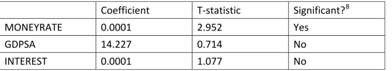
(25) on total output. This positive effect is shown in the VAR output, as the coefficient of RMSA is positive (14.277). Therefore, this change does follow the theoretical model. However, even though the coefficient is consistent in theory, it is not statistically significant at the 5% level. From the final results, we can conclude that while the theoretical model shows that there will be a positive impact on total output and real data does show this same effect, the data used in this test does not show significance in the change. 3.2.4. Effect on INTEREST Because RMSA is an exogenous variable, we are unable to see the impulse response of INTEREST to RMSA. Due to this, we cannot see by impulse response how the loan rate will change when a monetary policy is implemented. However, when looking at the coefficient of RMSA, we can see that it is positive (0.0001), but not statistically significant at the 5% level. This is similar to the case described in Figure 2.3. This shows that while the effect is positive, the data does not show a significant result.. 立. 政治大. ‧ 國. 學. ‧. 3.2.5. Considering 1997 Asian Financial Crisis and 2008 Global Financial Crisis. n. al. er. io. sit. y. Nat. The date range of this model includes two major financial crises, the 1997 Asian Financial Crisis, and the 2008 Global Financial Crisis. To see the effects of both crises, two dummy variables, one for the 1997 Asian Financial Crisis (D97) and the other for the 2008 Global Crisis (D08), were placed in the model as exogenous variables. When these dummy variables were added into the model, it showed that D97 is statistically significant for MONEYRATE only, D08 is statistically significant for GDPSA only, and D97 and D08 are not significant for INTEREST. This shows that the 1997 Asian Financial Crisis had a positive effect on the change in money rate, while the 2008 Global Financial Crisis had a negative effect on GDP. Also, the addition of these dummy variables into the model did not have a change on the statistical significance of RMSA to the dependent variables, as the coefficient for MONEYRATE is still statistically significant at the 5% level, while the coefficients for GDPSA and INTEREST were not statistically significant at the 5% level.. Ch. engchi. i n U. v. 3.3. Summary Table 3.1 shows the results of the coefficients, T-statistics and whether the coefficient is significant for the respective variables to RMSA: 21.

(26) Table 3.1. Dependent Variable Effects to Monetary Policy Shift Coefficient. T-statistic. Significant? 8. MONEYRATE. 0.0001. 2.952. Yes. GDPSA. 14.227. 0.714. No. INTEREST. 0.0001. 1.077. No. Source: EViews results From the above results, when there is a monetary policy shock, the money rate change is positive. This is similar to the scenario described in Figure 2.3, which is opposite of what the theoretical model showed. As theory has shown that for either the bond or loan rates to increase, a monetary tightening policy has to be implemented. However, actual data shows that the change is positive, meaning that a monetary expansion policy will lead to an increase in the overnight money rate. This result shows that Taiwan does not necessarily follow the traditional theory as a monetary policy change has a positive effect on the overnight money rate. Also, when looking at the change in the loan rate, the result shows that while the change is positive, it is not statistically significant. Although the data still shows that the change in positive, meaning that a monetary expansion policy will increase the loan rate which also contradicts the theoretical model, the change in not statistically significant at the 5% level. Although a monetary policy change will have a positive effect on the change in output, which is the same as the theoretical model, the data does not show significance at the 5% level. Table 3.2 shows the results of the coefficients, T-statistic, and significance for RMSA and the respective dummy variables to the other dependent variables:. 政治大. 立. ‧. ‧ 國. 學. n. er. io. sit. y. Nat. al. Ch. engchi. i n U. v. Table 3.2. Dummy Variables Results to Monetary Policy Shift MONEYRATE 910. GDPSA. INTEREST. 10366.50/0.451/N. -0.001/-0.016/N. D97. 1.082/4.197/Y. D08. 0.004/0.016/N. -84547.53/-3.392/Y 0.041/0.624/N. RMSA. 0.001/2.749/Y. 27.567/0.714/N. 0.0001/0.974/N. Source: EViews results After adding dummy variables for the two major financial crises during the model’s time frame, the 1997 crisis shows a statistically significant impact on the 8. 5% Level Coefficient/T-statistic/Significant at 5% level 10 Y=yes, N=no 9. 22.

(27) money rate, the 2008 crisis shows a statistically significant impact of total output, but neither shows a statistically significant impact on the loan rate. By looking at the coefficients, we can also see that the 1997 Crisis has a positive effect on the overnight money rate, showing that this crisis led to a jump in the money rate. Also, the 2008 Crisis has a negative effect on totally output, showing that this crisis led to a significant drop in total output. These results also show that the 1997 Crisis had a positive effect on total output and a negative effect on the loan rate, and the 2008 Crisis had a positive effect on the money rate and a positive effect on the loan rate, but these changes are not statistically significant. Also, even though the dummy variables have been added to the model, the signs of the coefficients and the significance levels of the policy variable are the same as the previous model when the dummy variables were not present.. 立. 政治大. ‧. ‧ 國. 學. n. er. io. sit. y. Nat. al. Ch. engchi. i n U. v. 23.

(28) Chapter 4: Conclusion Bernanke and Blinder (1988) showed in their paper that it is possible that the bond rate would increase in the event that income increases. Their model showed that the traditional IS-LM model that was already in place is inadequate in determining the exact effects of the bond rate when bank reserves increase. Once the loan market was placed into the IS-LM model to become their CC-LM model, a monetary expansionary policy would shift both the LM and CC curves, rendering the bond rate change undetermined. As described, there are cases where the bond rate could increase, decrease, or remain constant. These cases all depend on whether the LM curve shift is greater than the CC curve, the other way around, or if both curves shifts are equal to each other. Also, after solving the equations, Bernanke and Blinder also showed that the same monetary policy and resulting possible shifts in the LM and CC curves could result in different changes in the loan rate, too. With reserve money set as the exogenous policy variable, the model showed that a change in monetary policy will have a positive impact on the overnight rate. In previous theories, such a change would have an inverse impact on the overnight rate, but what is shown here is that Taiwan’s credit channel doesn’t necessarily follow the previous theoretical model. Also, the model showed that while there is a positive change in the loan rate, this change is insignificant. A possible explanation is that in Taiwan’s credit channel, the loan rate is unaffected by any monetary policy change. This means that any monetary policy change will only affect total output and the loan rate will remain constant. Finally, as the date range of this model covers the 1997 Asian Financial Crisis and the 2008 Global Financial Crisis, setting up a dummy variable to test the impact showed that the 1997 Crisis had a more significant impact on the money rate, while the 2008 Crisis had a more significant impact on total output. Even so, when looking at the changes in the economy based on an IS-LM model, it showed that when there is a monetary policy change, the changes in the money rate and output levels are of the same signs as is under the CC-LM model, suggesting that in Taiwan, the IS-LM changes also contradict the theoretical model. However, as this paper dealt with the overnight money rate as a substitute to the bond rate, it is possible that other close substitutes would show a different effect. Also, from Bernanke and Blinder’s paper, their money market equation includes a reserve requirement ratio, which can also change the bond rate when the ratio changes. Future studies can place an emphasis on this aspect, or a close substitute to the bond rate to determine how the credit channel operates in Taiwan.. 立. 政治大. ‧. ‧ 國. 學. n. er. io. sit. y. Nat. al. Ch. engchi. i n U. v. 24.

(29) References Bernanke, Ben and Alan Blinder, “Credit, Money, and Aggregate Demand.” American Economic Review, May 1988. Vol. 78, 435-439. Bernanke, Ben and Alan Blinder, “The Federal Funds Rate and the Channels of Monetary Transmission.” American Economic Review, Sept. 1992. Vol. 82, No. 4, 901-921. Bernanke, Ben and Mark Gertler, “Inside the Black Box: The Credit Channel of Monetary Policy.” Journal of Economic Perspective, Autumn 1995. Vol. 9, No. 4. 27-48.. 政治大. Cottarelli, Carlo and Angeliki Kourelis. “Financial Structure, Bank Lending Rates, and the Transmission Mechanism of Monetary Policy.” International Monetary Fund Staff Papers, Dec. 1994. Vol. 41, No. 4. 587-623.. 立. ‧ 國. 學. ‧. De Bondt, G.J., 2000. “Financial Structure and Monetary Transmission in Europe.” Edward Elgar, Cheltenham, UK.. er. io. sit. y. Nat. Hannan, Timothy H. and Allen N. Berger. “The Rigidity of Prices: Evidence from the Banking Industry.” American Economic Review, Sept. 1991. Vol. 81, No. 4. 938-945. Holtemoller, Oliver, “Further VAR Evidence for the Effectiveness of a Credit Channel in Germany.” Applied Economics Quarterly 49, 2003. Vol. 4, 359–381.. n. al. Ch. engchi. i n U. v. Hulsewig, Oliver and Eric Mayer, Timo Wollmerhauser, “Bank Loan Supply and Monetary Policy Transmission in Germany: An Assessment Based on Matching Impulse Responses.” Journal of Banking and Finance, 2006. Vol. 30, 2893-2910. Klein, Michael A., “A Theory of the Banking Firm.” Journal of Money, Credit, and Banking, May 1971. 205-218. Litterman, Robert B. and Laurence Weiss, "Money, Real Interest Rates, and Output: A Reinterpretation of Postwar U.S. Data," Econometrica, January 1985, Vol. 53, 129-156. McCallum, Bennett T., "A Reconsideration of Sims' Evidence Concerning 25.

(30) Monetarism," Economics Letters, 1983, Vol. 13 (2-3), 167-171. Sims, Christopher, "Macroeconomics and Reality," Econometrica, January 1980. Vol. 48, 1-48. 何棟欽，2001 年九月，「我國新台幣拆款利率與存、放款利率之關係」。中央銀行季刊，第二十三卷第三期。吳中書，陳立修，2004，「台灣總體經濟信用管道之探討」。2004 年亞太地區域研討會。. Data Sources. 立. Paper Sources. 政治大. ‧ 國. 學. ‧. 準備貨幣（月底數）(1993) “中華民國台灣地區金融統計月報” 民國八十三年一月, 中央銀行經濟研究處, March 2010.. er. io. sit. y. Nat. 準備貨幣（月底數）(1994) “中華民國台灣地區金融統計月報” 民國八十四年一月, 中央銀行經濟研究處, March 2010. 準備貨幣（月底數）(1995) “中華民國台灣地區金融統計月報” 民國八十五年一月, 中央銀行經濟研究處, March 2010.. n. al. Ch. engchi. i n U. v. 準備貨幣（月底數）(1996) “中華民國台灣地區金融統計月報” 民國八十六年一月, 中央銀行經濟研究處, March 2010. 準備貨幣（月底數） (1997) “中華民國台灣地區金融統計月報” 民國八十七年一月. 中央銀行經濟研究處, March 2010. 準備貨幣（月底數） (1998/6) “中華民國台灣地區金融統計月報” 民國八十八年一月. 中央銀行經濟研究處, March 2010. Electronic Sources 放款利率 (1992-2009), 中央銀行. 26.

(31) http://win.dgbas.gov.tw/dgbas03/bs7/calendar/calendar.asp?Page=1&Sel-Org=27&S hrField=ShrItm&KeyWrd=存款利率. [June 2010]. 國內生產毛額 (1992-2009), 行政院主計處. http://www.stat.gov.tw/lp.asp?ctNode=2404&CtUnit=1088&BaseDSD=7. [June 2010]. 準備貨幣（月底數）(1998/7-2009), 中央銀行經濟研究處. http://win.dgbas.gov.tw/dgbas03/bs7/calendar/calendar.asp?Page=1&SelOrg=27&ShrField=ShrItm&KeyWrd=準備貨幣. [June 2010] 拆款利率 (1992-2009), 中央銀行. http://win.dgbas.gov.tw/dgbas03/bs7/calendar/calendar.asp?Page=1&SelOrg=27&ShrField=ShrItm&KeyWrd=拆款利率. [March 2010].. 立. 政治大. ‧. ‧ 國. 學. n. er. io. sit. y. Nat. al. Ch. engchi. i n U. v. 27.

(32) Appendix A1. Chapter 2: Solving the model A1.1. Differentiating Loan, Money, and Goods Market Differentiating equation (2.1) and reorganizing dR to the right hand side, we get: �Lρ − m(i)R(1 − τ)λρ �dρ + [Li − λ(ρ, i)mi (1 − τ)R − m(i)R(1 − τ)λi ]di + Ly dy = λ(ρ, i)m(i)(1 − τ)dR ………………………………………………………………………….. (A1). Differentiating equation (2.2) and reorganizing dR to the right hand side, we get:. 政治大. Di di + Dy dy = (mi di)R + m(i)dR ……………………………………………………… (A2). 立. Differentiating equation (2.3) and reorganizing dR to the right hand side, we get:. ‧ 國. 學. ‧. −Yi di − Yρ dρ + dy = 0 ………………………………………………………………………. (A3). We reorganize A1, A2, and A3 to obtain the matrix K as described in equation (2.4). y. Nat. er. io. sit. A1.2. Differentiating the CC curve equation. Differentiating equation (2.13) and reorganizing dR to the right hand side, we. al. n. get:. Ch. engchi. i n U. v. �1 − Yρ ρy �dy − �Yi + Yρ ρi �di = Yρ ρR dR ……………………………..……………. (A4). We use equation (A4) to solve for the slope and shift magnitude of the CC curve. To solve for ρi , ρy , and ρR we reorganize equation (A1) to get dρ to one side, as shown in equation (A5) solve by differentiating i, y, and R to ρ, which equals equations (2.12a), (2.12b), and (2.12c) respectively.. �Lρ − m(i)R(1 − τ)λρ �dρ = −[Li − λ(ρ, i)mi (1 − τ)R − m(i)R(1 − τ)λi ]di − Ly dy − λ(ρ, i)m(i)(1 − τ)dR ……………………………………………….………………… (A5) 28.

(33) A1.3. Solving for Yi. From equation (2.6): |A| = {λ(ρ, i)m(i)(1 − τ) ∗ (Di − mi R) ∗ 1} + {Ly ∗ (−Yi ) ∗ m(i)}. − {[Li − λ(ρ, i)mi (1 − τ)R − m(i)R(1 − τ)λi ] ∗ m(i) ∗ 1} − {λ(ρ, i)m(i)(1 − τ) ∗ (−Yi ) ∗ Dy } ≶ 0. Assuming that |A| = 0, factoring out Yi we can get. −Yi �[Ly m(i)� + [λ(ρ, i)m(i)(1 − τ) ∗ Dy ]} − {[Li − λ(ρ, i)mi (1 − τ)R − miR1−τλimi+λρ,imi1−τDi−miR=0 ……………………… (A6). 政治大. For the terms {[Li − λ(ρ, i)mi (1 − τ)R − m(i)R(1 − τ)λi ]m(i)}, if we use the assumption described in footnote, 2, equation (A6) becomes. 立. ‧. ‧ 國. 學. −Yi �[Ly ∗ m(i)� + [λ(ρ, i) ∗ m(i) ∗ (1 − τ) ∗ Dy ]} − {[Li − m(i)R(1 − τ)λi ]m(i)} + {λ(ρ, i)m(i)(1 − τ)(Di − mi R)} = 0……………………………………………………………….. (A6a). io. Dy λ(ρ,i)m(i)R(1−τ)+m(i)(−Ly ). n. al. Ch. sit. λ(ρ,i)m(i)(1−τ)(Di −mi R)+(Li − m(i)R(1−τ)λi )m(i). }……………………………………..….. (A7). er. Nat. Yi = {−. y. From Footnote 5, we can see that. i n U. v. Substituting the complex version of ρR as shown in equation (2.12c), and reorganizing A7 we can get. engchi. Yi �Dy λ(ρ, i)m(i)(1 − τ) − m(i)Ly � − [λ(ρ, i)m(i)(1 − τ)] + [Li − λ(ρ, i)mi (1 − τR−miR1−τλi=0 ……………..………………………………………………………….. (A8). If we multiply out both equation (A6a) and equation (A8), we can see that they are equal to each other, which equals |A|.. 29.

(34) A2. EViews Output of the VAR Model A2.1. No Dummy Vector Autoregression Estimates Date: 08/23/10. Time: 16:29. Sample (adjusted): 1992Q4 2009Q4 Included observations: 69 after adjustments Standard errors in ( ) & t-statistics in [ ] GDPSA. MONEYRATE. 1.42E-06 3.56E-06 治政 (0.13358) (3.3E-07) 大(1.6E-06) [ 9.75349] [ 4.33555] [ 2.28334] 立 1.302901. 3.77E-07. (0.22820). (5.6E-07). (2.7E-06). [-1.82606]. [-0.39046]. [ 0.14143]. 0.034594. -1.38E-06. -4.41E-06. (0.16090). (3.9E-07). (1.9E-06). [ 0.21500]. [-3.49341]. [-2.34584]. n. al. INTEREST(-1). INTEREST(-2). INTEREST(-3). MONEYRATE(-1). Ch. 1.073010 e n gchi (54168.5) (0.13281). -6654.268. y. sit. io. -2.18E-07. ‧. Nat. -0.416700. er. GDPSA(-2). 學. ‧ 國. GDPSA(-1). GDPSA(-3). INTEREST. iv n U -0.676411 (0.63290). [-0.12284]. [ 8.07899]. [-1.06875]. -54603.22. -0.130322. 1.974232. (78429.7). (0.19230). (0.91637). [-0.69621]. [-0.67770]. [ 2.15442]. 39249.43. -0.062156. -1.051752. (40329.7). (0.09888). (0.47121). [ 0.97321]. [-0.62858]. [-2.23203]. -1847.986. 0.098909. 0.664559. (11686.4). (0.02865). (0.13654) 30.

(35) [-0.15813]. [ 3.45188]. [ 4.86703]. -7310.592. -0.009437. 0.180633. (12639.0). (0.03099). (0.14767). [-0.57841]. [-0.30453]. [ 1.22319]. 15995.75. 0.015196. -0.146047. (10873.2). (0.02666). (0.12704). [ 1.47112]. [ 0.57001]. [-1.14961]. 294608.0. 0.449450. -1.969468. (143755.). (0.35247). (1.67962). [ 2.04938]. [ 1.27514]. [-1.17257]. [ 0.34771]. [ 1.07730]. [ 2.95299]. 0.994752. 0.998599. 0.964079. 0.993847. 0.998357. 0.957886. 9.84E+10. 0.591298. 13.42714. 41180.32. 0.100969. 0.481147. 1099.393. 4133.342. 155.6648. -825.0897. 66.29742. -41.43616. 2470900.. 6.185072. 3.680435. 524993.9. 2.491093. 2.344565. Determinant resid covariance (dof adj.). 3366112.. Determinant resid covariance. 1999241.. MONEYRATE(-2). MONEYRATE(-3). C. 政治大 14.27787 0.000108 0.001417 立(41.0624) (0.00010) (0.00048). io. Akaike AIC Schwarz SC Mean dependent S.D. dependent. Log likelihood. y. a24.23449 -1.602824 1.519889 iv l C n h e n-1.246662 24.59065 g c h i U 1.876051. n. Log likelihood. sit. F-statistic. Nat. S.E. equation. er. Sum sq. resids. ‧. Adj. R-squared. 學. R-squared. ‧ 國. RMSA. -794.2559. Akaike information criterion. 23.97843. Schwarz criterion. 25.04692. 31.

(36) A2.2. With Dummy Vector Autoregression Estimates Date: 08/23/10. Time: 16:30. Sample (adjusted): 1992Q4 2009Q4 Included observations: 69 after adjustments Standard errors in ( ) & t-statistics in [ ]. GDPSA(-1). GDPSA. INTEREST. MONEYRATE. 1.258583. 1.44E-06. 3.44E-06. (0.12425). (3.3E-07). (1.4E-06). [ 10.1291]. [ 4.31600]. [ 2.47090]. 治 5.58E-07 政 -3.00E-07 大. -0.250355. (5.8E-07). (2.4E-06). [-1.15570]. [-0.51534]. [ 0.22991]. -0.052175. -1.34E-06. -4.47E-06. (0.15101). (4.1E-07). (1.7E-06). [-0.34552]. [-3.29033]. [-2.64081]. 3503.852. 1.069625. -0.244987. (50970.3). (0.13700). (0.57139). -47898.20. -0.135177. 1.569360. (73136.1). (0.19658). (0.81987). [-0.65492]. [-0.68763]. [ 1.91416]. 25452.80. -0.055517. -1.100686. (37528.3). (0.10087). (0.42070). [ 0.67823]. [-0.55037]. [-2.61632]. -4157.424. 0.099202. 0.441085. (11808.4). (0.03174). (0.13237). [-0.35207]. [ 3.12548]. [ 3.33212]. -6780.767. -0.009487. 0.236489. y. a[ 0.06874] [ 7.80725] [-0.42876] iv l C n hengchi U. n INTEREST(-3). MONEYRATE(-1). MONEYRATE(-2). sit. io INTEREST(-2). ‧. Nat. INTEREST(-1). er. GDPSA(-3). 學. 立(0.21663). ‧ 國. GDPSA(-2). 32.

(37) (11752.6). (0.03159). (0.13175). [-0.57696]. [-0.30032]. [ 1.79500]. 19822.16. 0.013849. -0.002626. (10532.5). (0.02831). (0.11807). [ 1.88200]. [ 0.48917]. [-0.02224]. 164173.6. 0.516179. -1.388874. (139489.). (0.37493). (1.56369). [ 1.17697]. [ 1.37672]. [-0.88820]. 27.56793. 0.000101. 0.001189. (38.5730). (0.00010). (0.00043). (23010.6). (0.06185). (0.25795). [ 0.45051]. [-0.01638]. [ 4.19714]. -84547.53. 0.041841. 0.004525. (24921.1). (0.06699). (0.27937). [-3.39260]. [ 0.62462]. [ 0.01620]. 0.995664. 0.998608. 0.972676. 38096.30. 0.102400. 0.427067. 1071.478. 3348.925. 166.1227. -818.5079. 66.53741. -31.99847. Akaike AIC. 24.10168. -1.551809. 1.304303. Schwarz SC. 24.52260. -1.130890. 1.725222. Mean dependent. 2470900.. 6.185072. 3.680435. S.D. dependent. 524993.9. 2.491093. 2.344565. Determinant resid covariance (dof adj.). 2192633.. Determinant resid covariance. 1172149.. MONEYRATE(-3). C. RMSA. 治 [ 2.74934] [ 0.71469] 政 [ 0.97436] 大立10366.50 -0.001013 1.082664. S.E. equation F-statistic Log likelihood. Log likelihood. y. sit. a0.994734 0.998310 0.966821 iv l C n h e n 0.587199 8.13E+10 g c h i U 10.21361. n. Sum sq. resids. er. io. Adj. R-squared. ‧. Nat R-squared. 學. D08. ‧ 國. D97. -775.8353. Akaike information criterion. 23.61842. Schwarz criterion. 24.88117 33.

(38) 立. 政治大. ‧. ‧ 國. 學. n. er. io. sit. y. Nat. al. Ch. engchi. i n U. v. 34.

(39)