國立交通大學
機械工程研究所
碩士論文
Development of a Parallel adaptive Mesh Refinement
Module for 3-D Unstructured Grid and Its Applications in
DSMC Method
平行化三維非結構性網格調適加密模組之發展及
其在直接蒙地卡羅法上之應用
研究生:鄭淵文
指導教授:吳宗信 博士
中華民國九十三年七月
平行化三維非結構性網格調適加密模組之發展及
其在直接蒙地卡羅法上之應用
Development of a Parallel adaptive Mesh Refinement Module for 3-D
Unstructured Grid and Its Applications in DSMC Method
研
究 生:鄭淵文
Student:
Yuan-Wen Jeng
指導教授:吳宗信
博士 Advisor:Dr. Jong-Shinn Wu
國 立 交 通 大 學
機械工程研究所
碩 士 論 文
A Thesis
Submitted to Institute of Mechanical Engineering Collage of
Engineering
National Chiao Tung University
In Partial Fulfillment of the Requirements
for the degree of
Master of Science
In
Mechanical Engineering
July 2004
Hsinchu, Taiwan, Republic of China
誌謝
首先對吳宗信老師這兩年來對於學生不厭其煩的給予耐心的指導與鼓勵, 致上莫大的感謝。使學生在這期間於各個方面都有不少的成長與歷練,並能於最 後順利的畢業。並在此一併感謝於碩士論文口試時,花費不少時間及精力於學生 論文的傅武雄教授、鄭金祥教授及郭添全博士,使得學生的論文有不少的改進。 在這兩年的求學生涯中,遇到不少困難與挫折,多虧實驗室中的許佑霖、曾 坤樟、邵雲龍、連又永、周欣芸、李允民等學長姐及學弟妹們所給予的幫助,才 能一一度過。這兩年吳志輝、吳俊賢、陳永彬等同學與我一起互相鼓勵與幫助, 亦使我的碩士生涯增色不少,在此一併感謝。 最後深深的感謝我的家人,沒有他們的支持與鼓勵也就沒有這篇論文的產 生。 度過了這一階段,人生又到了另一個轉折點,希望在交大所接觸的每一個人 都能邁向一個更美好了未來。 鄭淵文 謹誌 甲申年七月於風城交大平行化三維非結構性網格調適加密模組之發展及
其在直接蒙地卡羅法上之應用
學生:鄭淵文 指導教授:吳宗信 國立交通大學機械工程研究所中文摘要
本研究完成平行化三維非結構性四面體網格調適加密模組之發展及其在直 接模擬蒙地卡羅(DSMC)法上之應用。眾所皆知,假如需要網格來解流場,則不論 是使用粒子性或連續性的數值解法都非常需要一個好的網格分布。然而,在解求 得之前,好的網格分布一般來說是無法預測得知的。因此,在計算過程中一般需 要利用網格調適來得到一個最理想的網格。就穩態流場而言,較明智的做法是先 使用一個較粗糙的網格,再根據依此網格所得之流場結果去加密網格。然後將此 程序反覆執行直到滿足某一標準為止。在本論文中將延續先前實驗室已有之單機 三維非結構性四面體網格調適加密模組的成果,將其延伸為平行化可調性網格調 適加密模組(parallel adaptive mesh-refining, PAMR),並在通用的分散式記憶體電 腦群上運行,例如個人電腦叢集系統。在此PAMR模組中使用一個在不同作業系 統及硬體間具高移植性的標準MPI作為介面。最後,為了在運算時可以正確地將 網格加密,所以將此PAMR模組與先前發展的平行化直接蒙地卡羅法程式(PDSC) 結合。利用於計算在不同攻角時超高音速氮氣流過一個70°角的鈍圓錐體的流場以展示PAMR模組應用在粒子性方法上的性能。計算結果顯示將比以較粗略的網 格所計算出來的結果更接近實驗數據。
Development of a Parallel Adaptive Mesh Refinement Module for 3-D
Unstructured Grid and Its Applications in DSMC Method
Student: Yuan-Wen Jeng Advisor : Dr. Jong-Shinn Wu
Institute of Mechanical Engineering National Chiao Tung University
ABSTRACT
Development of a parallel adaptive mesh-refining (PAMR) module for three-dimensional unstructured tetrahedral mesh and its application in the direct simulation Monte Carlo (DSMC) method is reported. It is well known that numerical solution of either particle method or continuum method depends strongly upon the quality of mesh distribution if mesh is needed in the solution procedures. However, it is generally not known in priori before the solution is obtained. Thus, mesh adaptation is generally required to obtain an optimum mesh for computation. For steady-state flow problem, the general wisdom is to use coarser grid at first, then to refine the grid adaptively according to the solution on the coarser grid. The above procedure is then repeated until some criterion is satisfied. In the current thesis, we have continued previous efforts in our laboratory to extend the serial mesh-refining module for three-dimensional unstructured tetrahedral mesh into a parallel adaptive mesh-refining (PAMR) module on general memory-distributed machines, such as
is used to possess high portability between various operating system and hardware. Finally, this PAMR is incorporated into a previously developed parallel direct simulation Monte Carlo code (PDSC) to truly refine the mesh during the runtime. Hypersonic nitrogen flows over a 70° blunt cone (Kn∞=0.0108) at various angles of
attack are used to demonstrate the capability of the PAMR in the particle method. Computational results are compared more favorably with available experimental data for refined mesh than those for coarse mesh.
TABLE OF CONTENTS
中文摘要... I ABSTRACT... III TABLE OF CONTENTS...V LIST OF TABLES... VI LIST OF FIGURES ...VII
CHAPTER 1 INTRODUCTION ...1 1.1 Motivation...1 1.2 Background...3 1.2.1 Grid System in DSMC...3 1.2.2 Mesh Refinement in DSMC...5 1.3 Literature survey ...7
1.3.1 Serial Mesh Refinement for Unstructured Grid...7
1.3.2 Parallel Mesh Refinement...9
1.3.3 Development of Mesh Refinement at MuST Laboratory ...10
1.4 Objectives and Organization of the Thesis ...11
CHAPTER 2 NUMERICAL METHOD...12
2.1 MESH REFINEMENT ...12
2.1.1 The Basic Algorithm...12
2.1.2 Cell Quality Control...13
2.1.4 Surface Representation ...15
2.1.4 Procedures of Serial Mesh Refinement...15
2.1.5 Parallel Implement ...16
2.1.6 Procedures of Parallel Mesh Refinement...16
2.2 Parallel DSMC Method with Mesh Refinement...20
2.2.1 The DSMC Method...20
2.2.2 Parallel DSMC Method(PDSC)...21
2.2.3 Refinement Parameter and Criteria...23
2.2.4 Parallel DSMC Method with Mesh Refinement...25
CHAPTER 3 RESULTS AND DISCUSSIONS ...27
3.1 Hypersonic flow over a 70o blunt cone...27
3.2 Test for cell quality control ...27
3.3 Parallel Performance Evaluation...28
CHAPTER 4 CONCLUSIONS...29
CHAPTER 5 FUTURE WORK ...30
LIST OF TABLES
Table 1 Timing (seconds) for different processor numbers ...37 Table 2 Different refined level mesh for a hypersonic flow over 70o blunt cone with attack angle of 100. (Kn=0.0108)...38 Table 3 Comparison between experimental data and simulation data for different
refined level mesh for a hypersonic flow over 70o blunt cone with attack angle of 100. (Kn=0.0108) ...39
LIST OF FIGURES
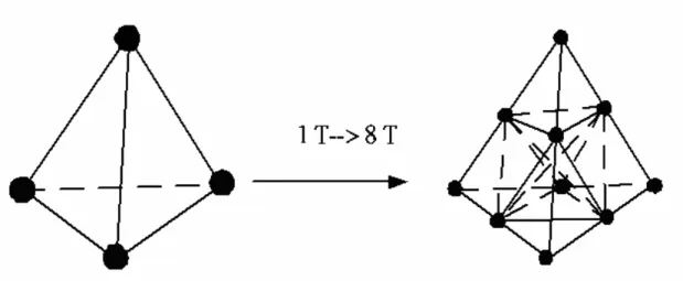
Figure 1 Isotropic mesh refinement of tetrahedral mesh. (T: Tetrahedron ) ...40
Figure 2 Mesh refinement rules for two-dimensional triangular cell ...41
Figure 3 Schematic diagram for mesh refinement rules of tetrahedron...42
Figure 4 Schematic diagram of the proposed cell quality control ...43
Figure 5 Schematic diagram of typical of cell quality control...44
Figure 6 Schematic diagram of simple cell quality control by Wu et al. [2004a] ....45
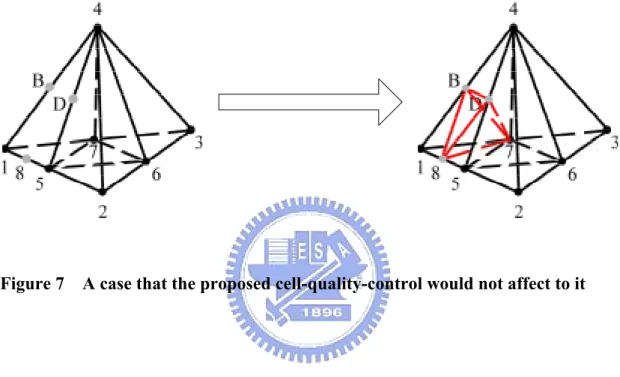
Figure 7 A case that the proposed cell-quality-control would not affect to it...46
Figure 8 Simplified flow chart of the serial mesh refinement. ...47
Figure 9 Flow chart of parallel mesh refinement module...48
Figure 10 Flow chart of module I (add nodes on cell edges)...49
Figure 11 Flow chart of serial DSMC method...50
Figure 12 Simplified flow chart of the parallel DSMC method (PDSC)...51
Figure 13 Coupled PDSC-PAMR Method...52
Figure 14 Sketch of a hypersonic flow over 70o blunt cone ...53
Figure 15 Original mesh of a hypersonic flow over 70o blunt cone with attack angle of 100...54
Figure 16 Level 1 refined mesh of a hypersonic flow over 70o blunt cone with attack angle of 100. ...55
Figure 17 Level 2 refined mesh of a hypersonic flow over 70o blunt cone with attack angle of 100. ...56
Figure 18 Level 3 refined mesh of a hypersonic flow over 70o blunt cone with attack angle of 100. ...57
Figure 19 Normalized density of original mesh of a hypersonic flow over 70o blunt cone with attack angle of 100. (Kn=0.0108) ...58
Figure 20 Normalized temperature of original mesh of a hypersonic flow over 70o blunt cone with attack angle of 100. (Kn=0.0108)...59
Figure 21 Streamlines of original mesh of a hypersonic flow over 70o blunt cone with attack angle of 100. (Kn=0.0108)...60
Figure 22 Mach number of original mesh of a hypersonic flow over 70o blunt cone with attack angle of 100. (Kn=0.0108)...61
Figure 23 Normalized density of level 3 refined mesh of a hypersonic flow over 70o blunt cone with attack angle of 100. (Kn=0.0108)...62
Figure 24 Normalized temperature of level 3 refined mesh of a hypersonic flow over 70o blunt cone with attack angle of 100. (Kn=0.0108)...63
Figure 25 Streamlines of level 3 refined mesh of a hypersonic flow over 70o blunt cone with attack angle of 100. (Kn=0.0108) ...64
Figure 26 Normalized Mach number of level 3 refined mesh of a hypersonic flow
over 70o blunt cone with attack angle of 100. (Kn=0.0108) ...65
Figure 27 Surface mesh distribution for a supersonic flow past a sphere ...66
Figure 28 Typical distribution surface mesh(1/16 domain) for a single jet case ...67
Figure 29 Timing for different modules of PAMR at different processors...68
CHAPTER 1 INTRODUCTION
1.1 Motivation
Computational cost using the direct simulation Monte Carlo (DSMC) method for molecular gas flows is generally very demanding, especially in near-continuum flow. In our Multiscale Science and Technology Laboratory (MuST), we have developed a parallel three-dimensional direct simulation Monte Carlo code (PDSC) [Wu et al., 2004b] to greatly shorten the computational time for resolving flow fields in rarefied gas dynamics. In this PDSC, 3-D unstructured tetrahedral mesh is used for particle tracking and properties sampling, by taking the advantages of more flexible parallel processing and easier treatment of complicated geometries of objects [Wu et al., 2004b]. Several advantages resulting from using unstructured mesh, rather than conventional structured mesh, include easier adaptation to complex geometries of objects, more flexible in parallel processing, easier implementation of mesh refinement and possible development of more practical hybrid DSMC-NS method [Wu et al., 2004b]. Details can be found in the reference [Wu et al., 2004b] and references cited therein.
It is also well known that numerical solution of either particle method or continuum method depends strongly upon the quality of mesh distribution if mesh is required in the solution procedures. However, it is generally not known in priori
before the solution is obtained. Thus, mesh adaptation is generally required to obtain an optimum mesh for computation. For steady problem, the general wisdom is to use coarser grid at first, then to refine the grid adaptively according to the solution on the coarser grid. The above procedure is then repeated until some criterion is satisfied. Hence, an adaptive mesh refinement technique is strongly needed. Previously, Kuo [Kuo, 2000] in our laboratory had developed an adaptive mesh-refining (h-refinement) module using two-dimensional unstructured grid in the DSMC method. Later, Wu [Wu, 2002] had successfully extended the two-dimensional mesh-refining module into a three-dimensional module for hybrid grid system (tetrahedral and hexahedral) and had applied this in the parallel three-dimensional DSMC computation. Computational results using adaptive refined mesh did show improvement in accuracy over coarse mesh, which encourages further use of adaptive mesh refinement.
However, there exist two disadvantages in the serial version of mesh-refining module. First, the mesh refinement has to be done decoupling from the DSMC computation. That is one has to compute the flow field using DSMC and then, based on the results output from the DSMC, one refine the mesh separately by stopping the DSMC code. With the refined mesh, then we restart the DSMC computation. The above procedure is repeated manually until some refinement criteria are satisfied. Second, the serial version of the mesh-refining module is not able to handle or
becomes very slow when the grid size is over some range, which is limited by the local RAM size of a computer. Thus, parallel implementation of the three-dimensional adaptive mesh-refining module, termed as “PAMR”, and incorporation of the PAMR module into the PDSC is strongly required in large-scale, three-dimensional DSMC computation.
1.2 Background
1.2.1 Grid System in DSMC
The DSMC method has been first developed to compute the hypersonic flow by Bird [1976] in late 1950s. Since then it has become the de-facto computational technique to deal with rarefied gas dynamics, including gas flows around spacecraft [Boyd and Stark, 1990; Boyd et al., 1992; Boyd et al., 1994], vacuum technology [Lee and Lee, 1996a; Lee and Lee, 1996b] and, recently, the micro-scale gas flows [Piekos and Breuer, 1996; Nance et al., 1998; Wu et al., 1999], etc. This method requires the introduction of computational cells (meshes) similar to those in Computational Fluid Dynamics (CFD), however, the cells are used for selecting collision partners, sampling and averaging the macroscopic flow properties. Many physical problems involve very complicated geometry and, hence, the generation of an appropriate mesh becomes a very demanding and time consuming task. Generally, the mesh used for final computation is obtained through trial and errors. In addition,
the sizes of cell used in the DSMC method have to vary according to the density and gradients of flow properties or have to be refined near the body surface to obtain accurate prediction of pressure and heat transfer, however, these are not known as a priori in general.
Most applications of DSMC applied structured meshes [Bird, 1994], in the physical space. For problems with complicated geometry, multi-block meshing techniques were developed first by Bird, which involved two steps: dividing the flow field into several blocks followed by discretizing each block into quadrilateral (2-D) or cubic (3-D) meshes. Subsequent research has been directed to develop alternative meshing techniques such as the coordinate transformation method by Merkle [1958], the body-fitted coordinate system by Shimada and Abe [1989] and the transfinite interpolation method by Olynick et al. All of them still used structured grids. It is much easier to program the code using structured grids; however, it requires tremendous problem specific modification. To alleviate such restriction and the easiness of applying adaptive mesh, unstructured mesh system is one of the best choices, although might be computationally more expensive.
And, unstructured mesh has two major advantages over structured mesh for solving computational problems. First, unstructured mesh able efficient mesh generation around highly complex geometries. Second, appropriate unstructured-grid
data structures facilitate the rapid insertion and deletion of points to allow the mesh to locally adapt to the solution. Boyd and his coworkers [1990; 1992; 1994] has applied such technique to compute the thruster plume produced by spacecraft and found that the results are very satisfactorily. In addition, several studies [Piekos and Breuer, 1996; Wu et al., 1999] have used such technique to compute micro-scale flows such as micro-channel, micro-nozzle and micro-maniflod.
1.2.2 Mesh Refinement in DSMC
For the past decade, the development of CFD using adaptive unstructured meshes has greatly extended the capability of predicting complex flow fields. Several adaptive mesh techniques have been developed to increase the resolution of “important” region and decrease the resolution of “unimportant” region within flow field [Powell and Roe, 1992; Kallinderis and Vijayan, 1993]. However, the corresponding development in the particle method, such as the DSMC method, is not as popular as expected.
However, it is very often that property variation in rarefied gas dynamics is large, for example, in hypersonic flows or vacuum pumping flows, which requires non-uniform mesh for resolving the flow field. Or equivalently, the cell size in DSMC has to be much smaller than the local mean free path for justifying the decoupling of particle movement and collision inherited in the DSMC method.
Adaptive mesh technique in the DSMC method not only improves the flow field resolution without increasing the computational cost, but also equalizes the statistical uncertainties in the averaging process to obtain macroscopic quantities in each cell. Among the very few studies on this subject, Wong and Harvey [1994] has first applied solution-based, re-meshing adaptive grid technique in unstructured meshes to study the hypersonic flow field with highly non-uniform density involving shock. Cybyb et al. [1995] have developed technique using the Monotonic Lagrangian Grid (MLG, hereafter) in the DSMC method, which provides a time-varying grid system that automatically adapts to local number densities within the flow field. However, the application of this MLG technique to external gas flows is not easy due to the problem of particle sorting in the designed scheme. Additionally, this technique highly restricts the size of time step as compared with the traditional DSMC method, which makes the steady-state solution prohibitively high. In addition to the applications in hypersonic flows, several gas flows, for example, in diffusion pumps and micro-nozzle, etc., all involve highly varying density in the flow field.
In our laboratory, C.-H. Kuo [2000] had developed a 2-D and unstructured adaptive mesh successfully, and used it in DSMC code to test a high-speed driven cavity flow and a hypersonic flow over a block. He had proven the 2-D unstuctured adaptive mesh generator could increase the solution accuracy and efficiency. Then,
Fu-Yuan Wu [Wu, 2002] had developed the 3-D unstructured mesh adaptation method (h-refinement) successfully and used in DSMC code to test on several benchmark problems. He also had proof the 3-D unstructured adaptive mesh generator would be efficient and robust.
1.3 Literature survey
1.3.1 Serial Mesh Refinement for Unstructured Grid
In general, mesh refinement can be categorized into three methods [Rausch et al., 1991]: (1) remeshing (mesh generation), (2) mesh movement, and (3) mesh enrichment (or h-refinement).
For the first method, a solution based on the initial mesh is obtained, and then the mesh is regenerated which the mesh points are more concentrated on where resolution of the solution is needed. This new mesh may contain more or fewer mesh points than the original mesh. There are many people had developed many different way to re-meshing a better mesh [Lee and Lo, 1995; Ruppert, 1995; Bond et al., 1996; Sullivan Jr. and Zhang, 1997; Zhu and Zienkiewicz, 1997; Manole et al., 2003]. And others had used it for Fluid Dynamics Simulation [Khokhlov, 1998; Cook, 1999; Felcman, 2003], DSMC [Garcia et al., 1999], Simulation of Laser Plasma Filamentation [Dorr, 2002], 3D Stress Analysis [Lee and Lo, 1997], MHD (magnetohydrodynamics) [Spicer et al., 1996; Ziegler, 1998].
For the second method, the total number of mesh points remains the same in the computational domain. It is common to use a spring analogy, in which the nodes of the mesh are connected by springs whose stiffness is proportional to certain measure of solution activity over the spring. The mesh points are moved closer into the region where solution gradients are relatively large. This method has a few people to use it for research about the numerical solution [Brackbill, 1993; Mackenzie and Robertson, 2000; Littlefield, 2001; Beckett et al., 2001; Huanga and Russellb, 2001; Tang et al., 2003].
For the final method, mesh enrichment, mesh points are added or embedded into the regions where relatively large solution gradients are detected, while the global mesh topology remains intact. It is generally regarded that mesh enrichment method has certain advantages over the first two methods [Rausch et al., 1991; Connell and Holms, 1994]. One of the most important advantages is that the mesh enrichment technique is in general many times faster and robust than the re-meshing technique [Connell and Holms, 1994]. In Ref. Rausch et al. (1991), it is mentioned that the disadvantage, however, is that the implementation of mesh enrichment involves a significant modification to existing numerical schemes due to the appearance of hanging nodes. This can be easily overcome, however, by some simple methods through the elimination of hanging nodes, as proposed by Kallinderis and Vijayan
[1993]. Therefore, h-refinement is using for many researches (For example, CFD [Löhner, 1995; Biswas and Strawn, 1998], solving evolution problems [Plaza et al., 2000], elastic-plastic problems [Cramer et al., 1999], LED-BGK solver [Kim and Jameson, 1998], Poisson-Boltzmann Equation [Dyshlovenko, 2001], Euler equation [Zeeuw and Powell, 1993], dynamic strain localization [Deb et al., 1996]). In order to get a better mesh, some researches combine two techniques [Cao, 1998; katragadda and Grosse, 1996]. But it becomes complex. E. Kita and N. Kamiya[2001] had tested most of adaptive mesh refinement methods in boundary element, they thought h-refinement would be better for the reference value method, the error convergence method and the equilibrium criterion method.
1.3.2 Parallel Mesh Refinement
There are some studies for parallel adaptive mesh refinement, Özturan et al. [1994] developed a 2D unstructured mesh refinement code for parallel in 1994. Then, in 1999, a parallel 3D structured mesh refinement code with dynamic load balancing had developed by MacNeice et al. [2000]. Later, some parallel mesh refinement codes were developed. And, all of them are 3D unstructured mesh refinement code with dynamic load balancing [Leyland and Richter, 2000; Oliker et al., 2000]. Furthermore, one of them has the ability to do mesh smoothing and cell-quality control [Lou et al., 1998; Norton et al., 2001].
1.3.3 Development of Mesh Refinement at MuST Laboratory
In our Multiscale Science and Technology Laboratory, C.-H. Kuo [2000] had developed an adaptive mesh refinement schemes using unstructured grid in the two-dimensional Direct Simulation Monte Carlo (DSMC) method, and tested the proposed scheme for Argon gas using different types of mesh, such as triangular and quadrilateral or mixed, to a high-speed driven cavity flow and, then, a hypersonic flow over a block. The results show an improved flow resolution as compared with that of un-adaptive mesh. Finally, we have used triangular adaptive mesh to compute two near-continuum gas flows, including a supersonic flow over a cylinder and a supersonic flow over a flat plate with a 35° compression ramp. The results show fairly good agreement with previous studies. The results show an improved flow resolution as compared with that of un-adaptive mesh. Then, Fu-Yuan Wu [2002] also had developed an adaptive mesh refinement schemes using unstructured grid in the three-dimensional DSMC method and tested in the three-dimensional DSMC method for Argon gas using different types of mesh, such as tetrahedron, hexahedron, and pyramid or mixed, to a high-speed driven cavity flow and, then, a hypersonic flow over a sphere. The results also show the same thing that an improved flow resolution as compared with that of un-adaptive mesh.
1.4 Objectives and Organization of the Thesis
Based on previous reviews, the current objectives of the thesis are summarized as follows:
(1) To develop a parallel 3-D unstructured tetrahedral adaptive mesh-refining module(PAMR).
(2) To couple this PAMR with PDSC and test using hypersonic nitrogen flow past a 70° blunt cone at various angles of attack .
The organization of this thesis would be stated as follow: First is this introduction, followed by the numerical method. Next would be the Results and discussions, and finally the Conclusions and Future work.
CHAPTER 2 NUMERICAL METHOD
In this chapter, the parallel mesh refinement module would be introduced and the algorithm would be outlined. And in order to understand easily, two-dimensional mesh would be used to explain additionally. Then, the conventional DSMC method would be introduced roughly. It would couple with parallel mesh refinement module to test and verify.
2.1 MESH REFINEMENT
2.1.1 The Basic Algorithm
In the adaptive mesh refinement module, the data to record new added nodes is based on cell. In other words, every cell would only know new added nodes that belong to it. The number of added nodes is fixed in each processor. However, before to divide cells, the number of added nodes must be unique in all processors.
In this module, it needs a neighbor identifying arrays. This array defines the interfacial cell for each face. It would record the global cell number of interfacial cells for each face of the cell.
At each mesh refinement step, individual edges are marked for refinement, or no change, based on an error indicator calculated from the solution. These cells which need to be refined would add new nodes on each edge. They are called isotropic cells. For two-dimensional mesh, a parent cell [Kuo, 2000] is divided to form four child
cells. For three-dimensional mesh and tetrahedral cell, the parent cell is divided to form eight child cells, as show in Figure 1.
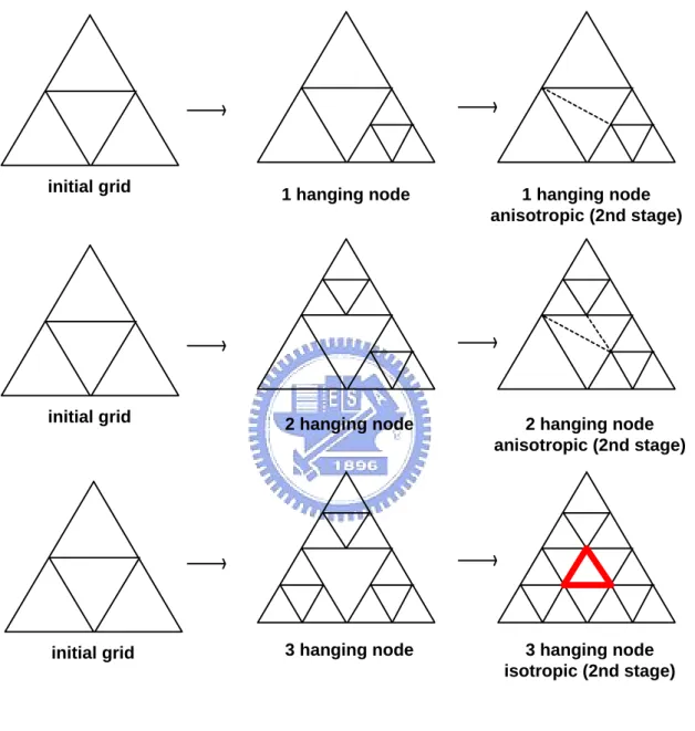
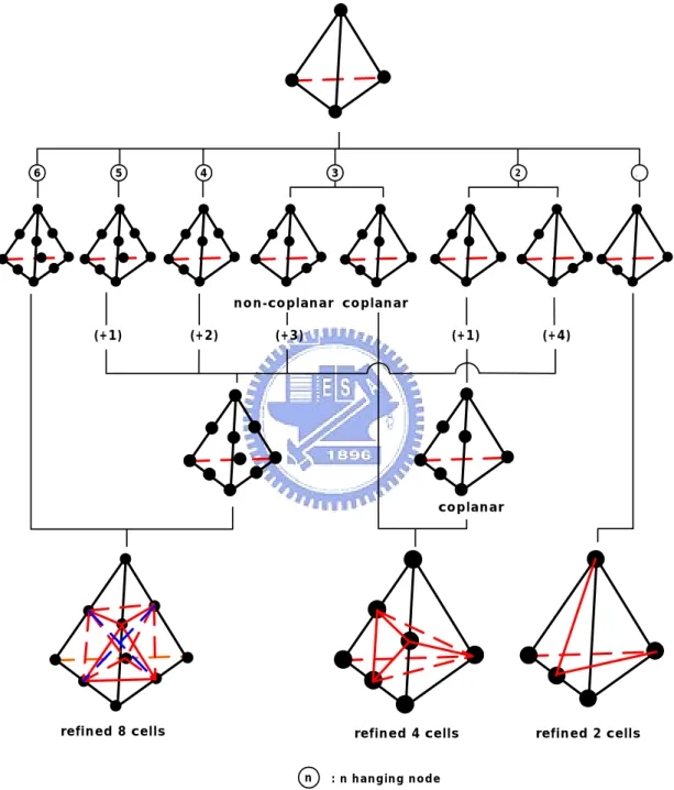
When isotropic cells add nodes on their edges, the cells neighbor them would appear one to three hanging nodes at the same time. The cells which have hanging nodes but not belong to isotropic cells are called anisotropic cells. In order to remove hanging nodes in anisotropic cells, it has some procedures to do. Using two-dimensional mesh as an example is shown in Figure 2. When hanging nodes appear in a triangular cell, the cell must be divided into different way. However, for three-dimensional mesh, the division is more complex. The division would consider the number and position of the hanging nodes, to decide whether to add new nodes to obey the refinement rules. There are three results. One is to divide into eight child cells. Another is to divide into four child cells. The other is to divide into two child cells. The detail refinement rules are be show in Figure 3.
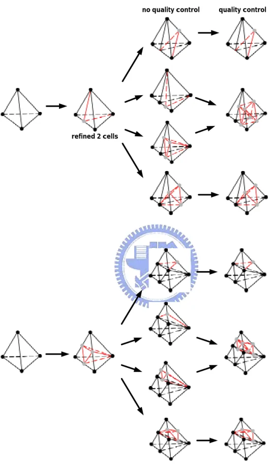
2.1.2 Cell Quality Control
A problem associated with repeated adaptive mesh refinement (AMR) operations. Then, most mesh smoothing schemes tend to change the structure of a given mesh to achieve the “smoothing effect” (a better aspect ratio) by rearranging nodes in the mesh. The changes made by a smoothing scheme, however, could modify the desired distribution of element density produced by the AMR procedure, and the cost of
performing a global mesh smoothing could be high. Alternatively, it is possible to prevent, or slow down, the degradation of cell quality during a repeated adaptive refinement process. The cell quality control scheme we have applied classifies elements based on how they will be refined. This allows us to avoid creating elements with poor aspect ratios during the refinement. After identifying those elements, we can refine them with a better refinement by contrast.
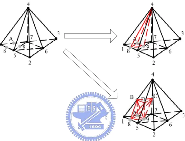
Detail rules are shown in Figure 4. For example, Figure 5 shows a typical cell (1-2-3-4). Because it is affecting by other cell, it has hanging nodes (8, 9, A). In order to handle hanging nodes, we connect nodes (8, 9, A) to node 4. But the aspect ratios of typical cells (1-4-8-A, 5-4-8-9 and 7-4-9-A) will be worse. However, if we add three nodes (B, C and D), and connect them with other nodes. Those eight child typical cells (4-B-C-D, 1-8-A-B, 5-8-9-D, 7-9-A-C, 8-9-A-B, 8-9-B-D, 9-A-B-C and 9-B-C-D) would have better aspect ratios.
However in some cases, previous developed cell-quality-control [Wu et al, 2004a] would not be effective that is shown in Figure 6. For example, as showed in Figure 7. At this situation, after the last refinement there are four child cells. But at this refinement, there are three hanging nodes appear on edges (8, B, D). While cells are divided, it will be divided to four child cells. And these four child cells will not get worse aspect ratios. And, it would get better aspect ratios. So cell-quality-control
will allow this division and not to affect it. 2.1.4 Surface Representation
If the boundaries of the computational domain are not straight, it is not sufficient to place the new node in the midway of the edge of the face of the parent cell. If this is done, it would dual to a rough piecewise representation of the original geometry results. What must be done is to move the new node location onto the real boundary contour surface. In the current implementation, it is assumed that the boundaries can be represented in parametric format. Specific neighbor identifiers are assigned to these non-straight boundary cells to distinguish from straight boundary cells. Whenever the boundary cells, which require mesh refinement, are identified as a non-straight boundary cell, the corresponding parametric function representing the surface contour are called in for mesh refinement to locate the correct node positions along the parametric surface.
2.1.4 Procedures of Serial Mesh Refinement
The corresponding flow chat is illustrated in Figure 8 (1) Flag the cells based on refinement criteria.
(2) Refine all the cells in which flag in Step 1 by conducting isotropic mesh refinement.
(3) Deal the interfacial cell. Check if there are any hanging nodes in the interfacial cells. If it does, then conduct anisotropic mesh refinement. Also
can remove the hanging node in the interfacial cells. (4) Deal the division of isotropic and anisotropic cells.
(5) Create and update the neighbor identifying arrays, coordinates, face numbers.
(6) Return to Step 1 if the accumulated adaptation levels are less than the preset maximum value.
(7) If the accumulated adaptation levels are greater than the preset value or no mesh refinement is required. Exit the adaptive mesh procedure.
2.1.5 Parallel Implement
In order to parallelize the mesh refinement module that is developed by F. Y. Wu [Wu, 2002], we use MPI to be the basic toll. And using Jostle to distribute meshes. Running the module to test and verity on PC Cluster belongs to our MuST laboratory. 2.1.6 Procedures of Parallel Mesh Refinement
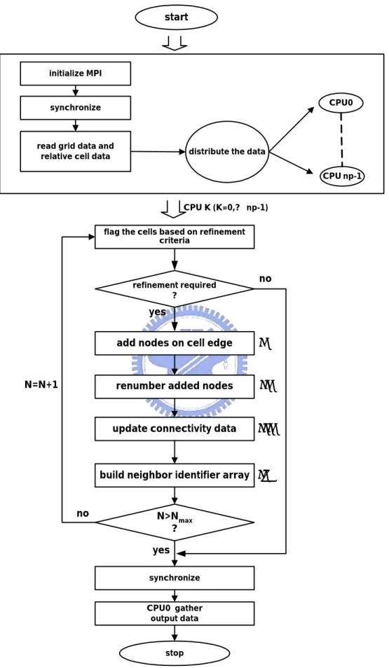
Figure 9 illustrates the flow chart of parallel adaptive mesh refinement (PAMR). Details are described step by step in the followings.
1. Set up initial grids and input data.
2. Initialize MPI and synchronize all processors to prepare for parallel computation
3. Read grid and relative cell data, and distribute them to every processor at the same time.
criterion calculated from the other module.
5. If there is no cell required to be refined, stop the module. Otherwise, go to next step.
6. Add new nodes to cells based on the module I., which is described in detail later. In this step, communications among processors are required.
7. Renumber all new added nodes in this step to “unify” the node numberings for all processors. Note that the node numberings for all original nodes are kept the same as those before refinement. In this step, communications among processors are required.
8. Update connectivity-related data to new child and old parent cells.
9. Build up new neighbor identifier array. Communication among processors is required in this step.
10. Decide if it reaches the preset maximum number of refinement. If it does, then go to next step, otherwise return to step 4.
11. Synchronize all processors
12. Host gathers all data and output the data at the same time.
In addition, all modules (I-IV in Fig. 9) in the core of the PAMR are explained in detail as follows in turn.
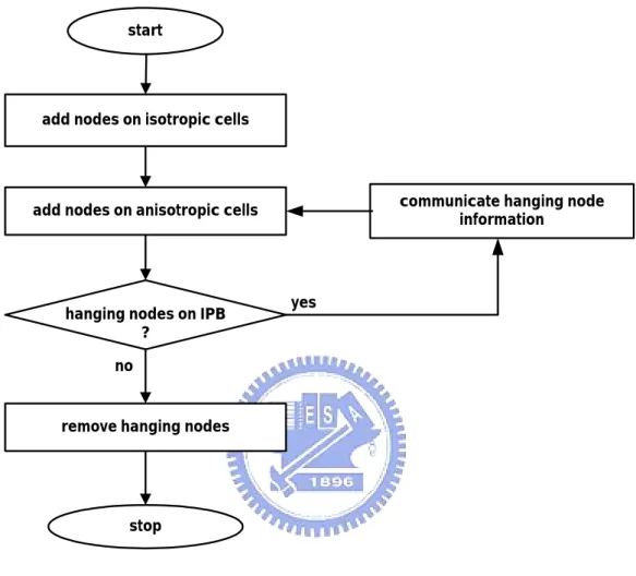
I-1. Add new nodes on all edges of “isotropic” cells that require refinement. These cells are called “isotropic” cells since it is refined from one cell to eight smaller cells.
I-2. Add new nodes to “anisotropic” cells, which may require further treatment in the following steps, if hanging nodes exits in these cells... Note that these cells are called “anisotropic” since they are not those cells originally require “isotropic” mesh refinement.
I-3. Communicate the hanging-node data to corresponding neighboring processors if the hanging nodes are located at the IPB (Interface Processor Boundary). If hanging-node data are received from other processors in this stage, then go back to Step I-2 for updating the node data. If there is no hanging-node data received at this stage, then move on to the next step.I-4. Remove hanging nodes based on refinement rules, if need to add new nodes go to I-2. If all cells obey the rules without to affect them, it mean all new nodes are be added.
I-4 . Remove hanging nodes based on Hanging-node Removal rules (Fig. 3). Go to Step I-2 to add new nodes if some more nodes addition is required. If there is no more node addition required, then ends this module execution.
Module II. Renumber added nodes:
II-1. Add up the number of the new added nodes in each processor, excluding those on the IPB.
II-2. Communicate this number to all processors. These are used to add up the total number of added nodes in the interior of all processors.
II-3. Renumber those added nodes in the interior of the processor according to results from Step-II-2.
II-4. Communicate data of added nodes on IPBs among all processors. II-5. Renumber the added nodes on IPBs on all processors.
Module III. Update connectivity data:
Form all new cells and define the new connectivity data for all cells. Module IV. Build neighbor identifier array:
IV-1. Reset the neighbor identifier array.
IV-2. Rebuild the neighbor identifier array for all the cells based on the new connectivity data. Note that those nbr informations on faces of the cells on the IPBs are not rebuilt and require further treatment in the next step.
IV-3. Record the neighbor identifier arrays that are not built in Step-IV-2, which the neighbor of the interested cell locates in the neighboring
processor.
IV-4. Broadcast all the recorded data in Step-IV-3 to all processors.
IV-5. Build the nbr information on the IPBs, considering the overall connectivity data structure.
2.2 Parallel DSMC Method with Mesh Refinement
2.2.1 The DSMC Method
The basic idea of the DSMC method is to calculate practical gas flows through the use of no more than the collision mechanics. The molecules move in the computational domain so that the physical time is a parameter in the simulation and all flows are computed as unsteady flows. An important feature of DSMC is that the molecular motion and the intermolecular collisions are uncoupled over the time intervals that are much smaller than the mean collision time. Both the collision between molecules and the interaction between molecules and solid boundaries are computed on a probabilistic basis and, hence, this method makes extensive use of random numbers. In most practical applications, the number of simulated molecules is extremely small compared with the number of real molecules. The details of the procedures, the consequences of the computational approximations can be found in Bird (1994); thus, it is only briefly described here for brevity. In brief summary, general procedure of the DSMC method consists of four major steps: moving,
indexing, collision and sampling, as shown in Figure 11. 2.2.2 Parallel DSMC Method(PDSC)
The DSMC algorithm is readily parallelized through physical domain decomposition. The cells of the computational grid are distributed among the processors. Each processor executes the DSMC algorithm in serial for all particles and cells in its domain. Data communication occurs when particles cross the domain (processor) boundaries and are then transferred between processors. Figure 12 illustrates a simplified flow chart of the 3-D parallel DSMC method. Procedures can be found in Lian’s MS thesis [Wu, J.-S. 2003] and are not repeated here in detail. First, we construct an unstructured tetrahedral using a commercial meshing tool. The output grid data are then processed using a conversion program to transform them into a globally sequential but locally unstructured mesh data conforming the partitioning information. In addition, a processor neighbor-identifying array is created for each processor, which is used to identify the surrounding processors due to the unstructured format of the processor distribution in the domain. From previous practical experience, the maximum numbers of processor neighbor are on the order of ten; therefore, the increase of memory cost is negligible. The resulting globally sequential but locally unstructured mesh data is then imported into the parallel DSMC code.
After reading the mesh data on a master processor (cpu0), the mesh data are then distributed to all other processors according to the predetermined domain decomposition. All the particles on each processor then start to move as in sequential algorithm. The particle data are sent to a buffer and is numbered sequentially when hitting the inter-processor boundary (IPB) during its journey within a simulation time step. After all the particles on a processor are moved, the destination processor for each particle in the buffer is identified via a simple arithmetic computation, owing to the approach adopted for the cell numbering, and are then packed into arrays. Considering communication efficiency the packed arrays are then sent as a whole to its surrounding processors in turn based on the tagged numbers. Once a processor sends out all the packed arrays, it waits to receive the packed arrays from its surrounding processors in turn. This “send” and “receive” operation serves practically as a synchronization step during each simulation time step. Received particle data are then unpacked and each particle continues to finish its journey for the remaining time step. The above procedures are repeated twice since there might be some particles cross the IPB twice during a simulation time step.
After all particles on each processors have come to their final locations at the end of a time step, the program then carries out the indexing of all particles and the collisions of particles in each computational cell on each processor as usual in a
sequential DSMC code. The particles in each cell are then sampled at the preset appropriate time.
Higher parallel efficiency can only be achieved if communication is minimized and the computational load is evenly distributed among processors. To minimize communication for between processors, the spatial domain decomposition should adapt according to the workload distribution as simulation continues, which requires dynamic domain decomposition. For the DSMC algorithm, the workload ( or equivalently particle numbers) on each processor changes frequently, especially, during the transient period of a simulation, while the workload attains a roughly constant value during steady-state sampling.
2.2.3 Refinement Parameter and Criteria
All mesh refinement methods need some means to detect the requirement of local mesh refinement to better capture the variations of the flow fields and hence to obtain more accurate numerical solutions. This also applies to DSMC. It is important for the refinement parameters to detect a variety of flow features but does not cost too much computationally. Often gradient of properties such as pressure, density or velocity is used as the refinement parameter to detect rapid changes of the flow-field solution in traditional CFD. However, by considering the statistical nature of the DSMC method, number density is adopted instead as the refinement parameter. Using
density as the refinement parameter in DSMC is justified since it is generally required that the mesh size be much smaller than the local mean free path to better resolve the flow features.
To use the density as an refinement parameter, a local cell Knudsen number is instead defined as 3 c c c V Kn = λ (1)
where λc is the local cell mean free path and Vc is the local cell volume. When
the mesh refinement module is initiated, local Knudsen number at each cell is computed and compared with a preset value, Kncc. If this value is less than the preset
value, then mesh refinement continues. If not, check the next cell until all cells are checked. This refinement parameter is expected to be most stringent on mesh refinement (more cells are added as compared with that based on property gradient); hence, the impact to DSMC computational cost may be high.
In addition, by considering the practical applications of mesh refinement in external flows, we have added another constraint, φ ≥ φ0, where φ, free-stream
parameter, is defined as (2) ρ ρ φ ρ∞ ∞ − =
particle rareness in the interfacial cells between refined and unrefined cells. 2.2.4 Parallel DSMC Method with Mesh Refinement
The mesh refinement procedure is performed after enough samples of data at each cell are gathered. As a rule of thumb, about 50,000 particles sampled in a cell are considered enough for the mesh refinement purpose. The mesh refinement module is initiated and checks through all the cells to determine if mesh refinement is required based on the specific refinement parameter, which will be explained later. If mesh refinement is conducted, associated neighbor identifying arrays are updated or created, coordinates and number of face for new cells are recorded, and sampled data on the coarse parent cell are redistributed (based on volume) to the fine child cells accordingly. Right after the mesh refinement, another mesh refinement process is initiated again and repeats the process described above until the prescribed maximum number of adaptation levels has been reached or no mesh enrichment is required for all the cells in the computational domain. Before processing the real parallel DSMC computation, all sampled data are reset to zero. Finally, the DSMC computation is then conducted on the final refined mesh to accumulate enough samples for obtaining the macroscopic properties in the cells.
The Figure 13, It shows coupled PDSC-PAMR method
(2) Proceed DSMC computation until enough sampled data are gathered at each cell.
(3) Compute the refinement parameters in each cell using Eqs. (1) and (2). (4) Refine all the cells in which the Knc is less than the preset Kncc and φ is
large than φ0 by conducting isotropic mesh refinement.
(5) Deal the interfacial cell. Check if there are any hanging nodes in the interfacial cells. If it does, then conduct anisotropic mesh refinement. Also create and update associated cell data. Unite if correspond the rule that can remove the hanging node in the interfacial cells.
(6) Deal the division of isotropic and anisotropic cells. The physical character of Knc is become twine, and the density is not change, respectively.
(7) Create and update the neighbor identifying arrays, coordinates, face numbers, and distribute sampled data to child cells,
(8) Return to (4) if the accumulated adaptation levels are less than the preset maximum value.
(9) If the accumulated refinement levels are greater than the preset value or no mesh refinement is required. Stop the refinement mesh procedure. (10) Adopt the adaptive data to run DSMC code again. The time step each
CHAPTER 3 RESULTS AND DISCUSSIONS
Several benchmark tests are conducted to verify the parallel adaptive mesh-refining module (PAMR). The part of blunt body is assisted by Lain Y-Y.
3.1 Hypersonic flow over a 70
oblunt cone
Hypersonic flow over a 70o blunt cone in the SR3 wind tunnel [James and
Joseph,1997, 8-10], shown in Figure 14. It is used to demonstrate the capability of the PAMR. The flow condition as followed: angles of attack=10o, N
2, M∞=20, Kn=0.0108,
Re=4116, T∞=13.6K, V=1502m/s. The original mesh and level 1-3 refined mesh is
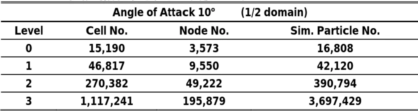
shown in Figure 15-18. Table 2 shows some properties for the case. Figure 19-26 show the density, temperature and streamlines of the flow for original mesh and level 3 refined mesh. In table 3 shows the simulation data compare with experimental data. It shows that as more mesh refining level is, the simulation data is more close to the experimental result. So the PAMR can improve the PDSC to better results.
3.2 Test for cell quality control
In Figure 27, it shows the difference between with cell-quality-control and without cell-quality-control. It is a supersonic flow over a sphere (Mach number = 4.2, Kn=0.1035, Argon, without cell quality control: 146,149cells, with cell quality control: 164,276cells). It can be observed easily. Without cell-quality-control there
are many cells with worse aspect ratio, but with cell-quality-control cells have better aspect ratio.
3.3 Parallel Performance Evaluation
In this section, a typical distribution surface mesh (1/16 domain) for a single jet is used to test performance of the PAMR module. The mesh is shown in figure 28. The mesh before refinement has 997,421 cells and 190,052 nodes. After refinement, it has 5,522,029 cells and 985,295 nodes.
The cost time for different processors number is shown in Table 1 and figure 29.Form they, we could see that the timing in part II- Renumber added nodes is much more than others. It must be improved. And from figure 30, we can see that when processor numbers is large, and the total timing is decrease. But while processor numbers increases to 16 processors, the total timing also increases. It means that the time saved from distribution to more processors is smaller than the time costs in communication. So, even they have more processors to join computation, it would not save time.
CHAPTER 4 CONCLUSIONS
In the current study, a parallel adaptive mesh-refining module (PAMR) for three-dimensional unstructured tetrahedral mesh and its application in the direct simulation Monte Carlo (DSMC) method is proposed. This module according to refinement criteria to refine the mesh. And, it has the cell quality control while refinement. This module is incorporated into PDSC to truly refine the mesh. Hypersonic nitrogen flows over a 70° blunt cone (Kn∞=0.0108) at various angles of
attack are used to demonstrate the capability of the PAMR.
In summary, major findings of the current research are listed as follows.
1. A parallel adaptive mesh-refining module (PAMR) for three-dimensional unstructured tetrahedral mesh is proposed and tested successfully on a hypersonic nitrogen flows case.
2. The proposed module can keep a good aspect ratio for the mesh by using cell quality control
3. Application of the propose module to a hypersonic nitrogen flows shows that it can improve the PDSC method to be close to experimental data.
CHAPTER 5 FUTURE WORK
From this study, future work is summarized as follows:1. From performance test, we can see that there is a bottleneck need to overcome.
2. Test with PDSC for more case or with other module to solve other problems.
REFERENCES
Bird, G. A., Molecular Gas Dynamics (Clarendon Press, Oxford, 1976)
Beckett, G., Mackenzie, J.A., and Robertson, M.L., “A Moving Mesh Finite Element Method for the Solution of Two-Dimensional Stefan Problems”, Journal of
Computational Physics, 168, P500–518, 2001
Bird, G. A., Molecular Gas Dynamics and the Direct Simulation of Gas Flows (Oxford University Press, New York, 1994)
Biswas, Rupak and Strawn, Roger C., “Tetrahedral and Hexahedral Mesh Adaptation for CFD Problems”, Applied Numerical Mathematics, 26, P135-151, 1998
Bond, T.J., Li, L.Y., Bettess, P., Bull, J.W. and Applegarth, I., “Adaptive Mesh
Refinement for Shells With Modified Ahmad Elements”, Computers & Structures, Vol. 61, No. 6, P1135-1141, 1996
Boyd, I. D. and Stark, J. P. W., “Modeling of a small hydrazine thruster plume in the transitionflow rehime,” J. Prop. Power 6, 121 (1990).
Boyd, I. D., Jafry, Y. and Beukel, J. W., “Particle simulation of helium microthruster flows,” J. Spacecraft Rockets 31, 271 (1994).
Boyd, I. D., Penko, P. F., Meissner, D. L. and DeWitt, K. J., ”Experimental and numerical investigations of low-densiity nozzle anplume flows of nitrogen,” AIAA Journal 30, 2453 (1992).
Brackbill, J.U., “An Adaptive Grid with Directional Control”, J. of Computational Physics, 108, P38-50, 1993
Cao, Thang, “Adaptive H-and H-R methods for Symm’s integral equation”, Compit. Methods Appl. Mech. Engrg, 162, P1-17, 1998
Connell, S.D. and Holms, D.G., “Three-Dimensional Unstructured Adaptive Multigrid Scheme for the Euler Equations,” AIAA Journal, 1994; 32:1626-1632.
Cook, Andrew W., “A Consistent Approach to Large Eddy Simulation Using Adaptive Mesh Refinement”, J. of Computational Physics, 154, P117-133, 1999
Cramer, H., Rudolph, M., Steinl, G. and Wunderlich, W., “A Hierarchical Adaptive Finite Element Strategy for Elastic Plastic problems”, Computers and Structures, 73, P61-72, 1999
Simulation Monte Carlo Model”, J. Computational Phys. , 122, P.323-334, 1995 Deb, Arghya, Prevost, Jean H. and Loret, Benjamin, “Adaptive Meshing for Dynamic Strain Location”, Comput. Methods Appl. Engrg. 137, P285-306, 1996
Dietrich, S. and Boyd, I., “Scalar and Parallel Optimized Implementation of the Direct Simulation Monte Carlo Method, ”J. Comp. Phys., Vol. 126, pp.328-342, 1996
Dorr, Milo R., Garaizar, F. Xabier, and Hittinger, Jeffrey A. F., “Simulation of Laser Plasma Filamentation Using Adaptive Mesh Refinement”, J. of Computational Physics, 177, P233-263, 2002
Dyshlovenko, Pavel, “Adaptive Mesh Enrichment for the Poisson-Boltzmann Equation”, Journal of Computational Physics 172, P198–208, 2001
Felcman, Jirı, “Grid Refinement/Alignment in 3D Flow Computations”, Mathematics and Computers in Simulation, 61, P317-331, 2003
Garcia, Alejandro L., Bell, John B., Crutchfield, William Y., and Alder, Berni J., “Adaptive Mesh and Algorithm Refinement Using Direct Simulation Monte Carlo”, J. of Computational Physics, 154, P134-155, 1999
Huanga, Weizhang and Russellb, Robert D., “Adaptive Mesh Movement — The MMPDE Approach and Its Applications”, Journal of Computational and Applied Mathematics, 128, P383–398, 2001
James N. Moss, Joseph M. Price, “Survey of Blunt Body Flows including wakes at Hypersonic Low-Density Conditions,” Journal of Thermophysics & Heat Transfer, Vol. 11, No. 3, pp. 321-329, 1997.
Kallinderis, Y. and Vijayan, P., “Adaptive Refinement-Coarsening Scheme for
Three-Dimensional Unstructured Meshes”, AIAA JOURNAL, Vol. 31, No. 8, August 1993.
Katragadda, P. and Grosse, I.R., “A Posteriori Error Estimation and Adaptive Mesh Refinement for Combined Thermal-Stress Finite Element Analysis”, Computers & Structures, Vol. 59, No. 6, P1149-1163, 1996
Khokhlov, A.M., “Fully Threaded Tree Algorithms for Adaptive Refinement Fluid Dynamics Simulations”, J. of Computational Physics, 143, P519-543, 1998
Kim, Chongam and Jameson, Antony, “A Robust and Accurate LED-BGK Solver on Unstructured Adaptive Meshes”, J. of Computational Physics, 143, P598–627, 1998
Boundary Element Method, an Overview”, Engineering Analysis with Boundary, 25, P479-495, 2001
Kuo, Chia-Hao, "The Direct Simulation Monte Carlo Method Using Unstructured Adaptive Mesh and Its Applications,", MS Thesis, NCTU, Hsinchu, Taiwan 29, Jun., 2000.
Lee, C.K. and Lo, S.H., “An Automatic Adaptive Refinement Procedure Using Triangular And Quadrilateral Meshes”, Engineering Fracture Mechanics, Vol. 50, No. 5/6, P671-686, 1995
Lee, C.K. and Lo, S.H., “Automatic Adaptive Refinement Finite Element Procedure for 3D Stress Analysis”, Finite Elements in Analysis and Design, 25, P135-166, 1997 Lee, Y. K. and Lee, J. W., “Direct simulation of compression characteristics for a simple drag pump model,” Vacuum 47, 807 (1996a).
Lee, Y. K. and Lee, J. W., “Direct simulation of pumping characteristics for a model diffusion pump,” Vacuum 47, 297(1996b).
Leyland, P. and Richter, R., “Completely Parallel Compressible Flow Simulations Using Adaptive Unstructured Meshes”, Comput. Methods Appl. Mech. Engrg. 184, P467-483, 2000
Littlefield, David L., “The Use of R-Adaptivity with Local, Intermittent Remesh For Modeling Hypervelocity Impact and Penetration”, International Journal of Impact Engineering, 26, P433-442, 2001
Löhner, Rainald, “Mesh Adaptation in Fluid Mechanics”, Engineering Fracture Mechanics, Vol. 50, No. 5/6, P819-847, 1995
Lou, John Z., Norton, Charles D., and Cwik, Thomas A., “A Robust and Scalable Software Library for Parallel Adaptive Refinement on Unstructured Meshes”, In 5th Intl. Symp. on Solving Irregularly Structured Problems in Parallel, Berkeley, CA 1998.
Mackenzie, J.A. and Robertson, M.L., ” The Numerical Solution of
One-Dimensional Phase Change Problems Using an Adaptive Moving Mesh Method”, J. of Computational Physics, 161, P537-557, 2000
MacNeice, Peter, Olsonb, Kevin M., Mobarry, Clark, Fainchtein, Rosalinda de and Packer, Charles, “PARAMESH: A parallel adaptive mesh refinement community toolkit”, Computer Physics Communications, 126, P330–354, 2000
Manole, Ovidiu, Labbé, Paul, Dompierre, Julien and Trépanier, Jean-Yves, “Anisotropic Hybrid Mesh Adaptation Using A Metric Field”, 16th AIAA Computational Fluid Dynamics Conference, 23-26, June, 2003
Merkle, C. L, “New Possibilities and Applications of Monte Carlo
Methods,“ Rarefied Gas Dynamics (ed. Belotserkovsk II), 13th International Symposium, pp. 333-348, 1985
Nance, R. P., Hash, D. B. and Hassan, H. A., “Role of boundary conditions in monte carlo simulation of microelectromechanical systems”, Journal of Thermophysics and Heat Transfer 12, Technical Notes, 447 (1998).
Norton, Charles D., Lou, John Z., and Cwik, Thomas. “Status and Directions for the PYRAMID Parallel Unstructured AMR Library”, In 8th Intl. Workshop on Solving Irregularly Structured Problems in Parallel (15th IPDPS), San Francisco, CA 2001. Oliker, Leonid, Biswas, Rupak and Gabow, Harold N., “Parallel Tetrahedral Mesh Adaptation with Dynamic Load Balancing”, Parallel Computing, 26, P1583-1608, 2000
Olynick, D. P., Moss, J. N. and Hassan, H. A., “Grid Generation and Application for the Direct Simulation Monte Carlo Method to the Full Shuttle Geometry,” AIAA Paper 90-1692.
Piekos, E. S. and Breuer, K. S., “Numerical modeling of micromechanical devices using the direct simulation monte carlo method”, Trans. ASME J. Fluids Eng. 118, 464 (1996).
Plaza, Angel, Padrón, Miguel A. and Carey, Graham F., “A 3D Refinement/ Derefinement Algorithm for Solving Evolution Problems”, Applied Numerical Mathematics, 32, P401-418, 2000
Powell, Kenneth G. and Roe, Philip L. “Adaptive-mesh algorithms for computational fluid dynamics”, Algorithmic Trends in Computational Fluid Dynamics, Springer Verlag Co, New York, 1992, P.301-337
Rausch, R.D., Batina, J.T. and Yang, H.T.Y., "Spatial Adaption Procedures on Unstrutuctured Meshes for Accurate Unsteady Aerodynamics Flow Computation," AIAA Paper No. 91-1106-CP, 1991.
Ruppert, Jim, “A Delaunay Refinement Algorithm for Quality 2-Dimensional Mesh Generation”, J. of Algorithms, 18. P548-585, 1995
in a Body-fitted Coordinate System,” Rarefied Gas Dynamics, Ed. Muntz et al., Progress in Astronautics and Aeronautics, pp. 258-270, AIAA, 1989.
Spicer, D.S., Zalesak, S.T., Löhner, R. and Curtis, S., “Simulation of The
Magnetosphere With A New Three Dimensional MHD Code and Adaptive Mesh Refinement: Preliminary Results”, Adv. Space Res. Vol. 18, No. 8, P(8)253-(8)262, 1996
Sullivan Jr., John M. and Zhang, James Qingyang, “Adaptive Mesh Generation Using A Normal Offsetting Technique”, Finite Elements in Analysis and Design, 25,
P275-295, 1997
Tang, H.Z., Tang, Tao and Zhang, Pingwen, “An Adaptive Mesh Redistribution Method for Nonlinear Hamilton–Jacobi Equations in Two- and Three-Dimensions”, Journal of Computational Physics, 188, P543–572, 2003
Vanderstraeten, D. and Keunings, R., “Optimized Partitioning of Unstructured Finite Element Meshes,” Intl. J. Num. Meth. Engng. 38(3), 433-450, 1995
Wang, L. and Harvey, J. K., “The Application of Adaptive Unstructured Grid Technique to the Computation of Rarefied Hypersonic Flows Using the DSMC Method,” Rarefied Gas Dynamics (ed. J. Harvey and G. Lord), 19th International Symposium, pp. 843-849, 1994.
Wu, Fu-Yuan, "The Three-Dimensional Direct Simulation Monte Carlo Method Using Unstructured Adaptive Mesh and It Applications", MS Thesis, NCTU, Hsinchu, Taiwan , July., 2002.
Wu, J.-S., Lee, Fred and Wong, S.-C., “Treatment of pressure related boundary
conditions in micromechanical devices using DSMC method,” AIAA Journal, October (1999). (submitted)
Wu, J.-S. and Lian, Y.-Y., "Parallel Three-Dimensional Direct Simulation Monte Carlo Method and Its Applications, " Computers & Fluids Volume 32, Issue 8 , Pages 1133-1160, September 2003.
Wu, J.-S., Tseng, K.-C. and Lian, Y.-Y., “Development of a General Parallel Direct Simulation Monte Carlo Code”, presented at 24th International Symposium on Rarefied Gas Dynamics, July 10-16, 2004, Bari, Italy.(2004a)
Wu, J-S, Tseng, K-C and Wu, F-Y, “Parallel Three-Dimensional DSMC Method Using Mesh Refinement and Variable Time-Step Scheme”, Computer Physics Communications, 2004 (accepted)(2004b)
Zeeuw, Darren De and Powell, Kenneth G., “An Adaptively Refined Cartesian Mesh Solver for the Euler Equations”, Journal of Computational Physics, 104, P56-68, 1993 Zhu, J. Z. and Zienkiewicz, O. C., "A Posteriori Error Estimation and
Three-Dimensional Automatic Mesh Generation", Finite Elements in Analysis and Design, 25, P167-184, 1997
Ziegler, Udo, “NIRVANA+: An Adaptive Mesh Refinement Code for Gas Dynamics and MHD”, Computer Physics Communications, 109, P111-134, 1998
Özturan, C., deCougny, H.L., Shephard, M.S. and Flaherty, J.E., “Parallel Adaptive
mesh refinement and redistribution on distributed memory computers”, Comput. Methods Appl. Mech. Engrg. 119, P123-137, 1994
Table 1 Timing (seconds) for different processor numbers
(Surface mesh for a single jet case, original mesh: cells:997,421. nodes: 190,052. level-1 refinement: cells:5,522,029. nodes:985,295.)
Processor NO. 2 4 8 16 Preprocessing 15.988 18.485 20.077 17.602 I 1564.7 499.08 659.9 491.86 II 14295 5360.4 5149.8 6922.2 III 1.35 2.072 2.174 2.399 IV 44.07 23.338 15.961 10.585 I. Add nodes on cell edges
II. Renumber added nodes III. Update connectivity data IV. Build neighbor identifier array
Table 2 Different refined level mesh for a hypersonic flow over 70o blunt cone with attack angle of 100. (Kn=0.0108)
Angle of Attack 10o (1/2 domain)
Level Cell No. Node No. Sim. Particle No.
0 15,190 3,573 16,808
1 46,817 9,550 42,120
2 270,382 49,222 390,794
Table 3 Comparison between experimental data and simulation data for different refined level mesh for a hypersonic flow over 70o blunt cone with attack
angle of 100. (Kn=0.0108) Angle of Attack 10o Level Cd Cl Cm 0 1.688(14.36%) -0.135(25.00%) -0.064(18.52%) 1 1.652(11.92%) -0.147(18.33%) -0.063(16.67%) 2 1.587(7.52%) -0.163(9.44%) -0.058(7.41%) 3 1.555(5.35%) -0.175(2.78%) -0.055(1.85%) Exp. Data 1.476 -0.18 -0.054
isotropic ( 1st stage) isotropic ( 2nd stage) anisotropic ( 2nd stage) initial grid initial grid initial grid 2 hanging node anisotropic (2nd stage) 3 hanging node isotropic (2nd stage) 1 hanging node anisotropic (2nd stage) 2 hanging node 3 hanging node 1 hanging node
refined 4 cells
refined 8 cells refined 2 cells
(+1) (+2) (+3) (+1) (+4) non-coplanar coplanar 6 5 4 3 2 1 coplanar : n hanging node (+n) : adding n nodes n
quality control no quality control
refined 2 cells
quality control no quality control
refined 2 cells
read grid data & related cell data
add nodes on isotropic cells refinement cells add nodes on anisotropic cells no
stop
start
refine all cells by refinement criteria
yes
advance mesh refinement ? update cell-related data
yes no
Figure 9 Flow chart of parallel mesh refinement module
CPU0 gather output data
flag the cells based on refinement criteria
renumber added nodes
synchronize
stop
start
add nodes on cell edge
refinement required ?
no
yes
update connectivity data
N>Nmax ? yes no
build neighbor identifier array
CPU K (K=0,? np-1)
N=N+1
distribute the data read grid data and
relative cell data synchronize CPU np-1 CPU0 initialize MPI I II III IV
Figure 10 Flow chart of module I (add nodes on cell edges)
remove hanging nodes
stop start
add nodes on isotropic cells
communicate hanging node information
hanging nodes on IPB ?
yes
no
Figure 11 Flow chart of serial DSMC method
read grid data
set initial state
move particles
entering new particles
collide particles
steady flow ?
sample flow field
sufficient sampling ?
Average samples and print out the data index particles start stop no no yes yes
Figure 12 Simplified flow chart of the parallel DSMC method (PDSC) (Wu et al. 2004b)
INITIALIZE MPI
READ GRID DATA
DISTRIBUTE THE DATA
MOVE PARTICLES
ENTER NEW PARTICLES
COLLIDE PARTICLES
MAIN CPU GATHER OUTPUT DATA CONVERT GRID DATA SYNCHRONIZE SYNCHRONIZE CPU1 CPU2 CPU np-1 CPU0
SAMPLE FLOW FIELD
RESET SAMPLING DATA NO YES YES NO YES NO REPARTITION THE DOMAIN RENUMBER CELLS LOAD BALANCING? STEADY FLOW? SUFFICIENT SAMPLING? STOP START COMMUNICATE PARTICLE DATA
Figure 13 Coupled PDSC-PAMR Method visual preprocessor stop PAMR mesh partition (weighting from PDSC) PDSC mesh partition
(weighting based on cell volume)
start (N=0) N< NMAX Refinement criteria satisfied ? no yes yes N=N+1
Figure 14 Sketch of a hypersonic flow over 70o blunt cone N2 M∞ = 20 T∞ = 13.6 K Tw = 300 K α=1
α
Figure 15 Original mesh of a hypersonic flow over 70o blunt cone with attack angle
Figure 16 Level 1 refined mesh of a hypersonic flow over 70o blunt cone with attack
Figure 17 Level 2 refined mesh of a hypersonic flow over 70o blunt cone with attack angle of 100.
Figure 18 Level 3 refined mesh of a hypersonic flow over 70o blunt cone with attack
Figure 19 Normalized density of original mesh of a hypersonic flow over 70o blunt
Figure 20 Normalized temperature of original mesh of a hypersonic flow over 70o
Figure 21 Streamlines of original mesh of a hypersonic flow over 70o blunt cone
Figure 22 Mach number of original mesh of a hypersonic flow over 70o blunt cone
Figure 23 Normalized density of level 3 refined mesh of a hypersonic flow over 70o blunt cone with attack angle of 100. (Kn=0.0108)
Figure 24 Normalized temperature of level 3 refined mesh of a hypersonic flow over 70o blunt cone with attack angle of 100. (Kn=0.0108)
Figure 25 Streamlines of level 3 refined mesh of a hypersonic flow over 70o blunt
Figure 26 Normalized Mach number of level 3 refined mesh of a hypersonic flow over 70o blunt cone with attack angle of 100. (Kn=0.0108)
(a)
(b)
Figure 27 Surface mesh distribution for a supersonic flow past a sphere (M∞=4.2, Kn∞=0.1035, Argon) (a)with cell quality control
(a)
(b)
Figure 28 Typical distribution surface mesh(1/16 domain) for a single jet case (Kn=0.001, Ps/Pb=150) (a)original mesh (997421 cells) (b)level-1 refined mesh (5522029 cells)
0. preprocessing
I. add node on cell edges II. renumber added nodes III. update connectivity data IV. build neighbor identifier array
Figure 29 Timing for different modules of PAMR at different processors
0
2000
4000
6000
8000
10000
12000
14000
16000
0
I
II
III
IV
Time (s)
2
4
8
16
0 2000 4000 6000 8000 10000 12000 14000 16000 18000 2 4 8 16 Processor numbers Time(s)
![Figure 6 Schematic diagram of simple cell quality control by Wu et al. [2004a]](https://thumb-ap.123doks.com/thumbv2/9libinfo/8433421.181358/56.892.134.686.103.1045/figure-schematic-diagram-simple-cell-quality-control-wu.webp)