多個低階決策單位二階層規劃應用之研究－以預算分配為例

國

立

交

通

大

學

科技管理研究所

博

士

論

文

多個低階決策單位二階層規劃應用之研究

－以預算分配為例

Application of a Bilevel Multi-Follower

Decision-Making Model for Budget Allocation

Problems

研究生：楊有恆

指導教授：虞孝成教授

多個低階決策單位二階層規劃應用之研究

－以預算分配為例

Application of a Bilevel Multi-Follower

Decision-Making Model for Budget Allocation

Problems

研究生：楊有恆 Student: Yeou-Herng Yang

指導教授：虞孝成教授 Advisor: Dr. Hsiao-Cheng Yu

國 立 交 通 大 學

科技管理研究所

博 士 論 文

Dissertation

Submitted to Institute of Management of Technology College of Management

National Chiao Tung University in partial Fulfillment of the Requirements

for the Degree of Ph. D in

Management of Technology October 2011

Hsinchu, Taiwan, Republic of China

多個低階決策單位二階層規劃應用之研究

－以預算分配為例

研究生：楊有恆 指導教授：虞孝成教授

國立交通大學科技管理研究所博士班

摘 要

過去許多學者們為解決當時社會上所發生的一些經濟與管理問題，促使了數學規劃 相關理論的發展與突破，而層級結構的規劃模式可以清楚描繪出組織體系之間的決策模 式與運作過程，促使多層級規劃的概念逐漸展開。而二階層規劃係為解決二個層級結構 間分權式決策的尋優問題，可視為一個多層級規劃的特殊型式，在上階層之決策者稱為 領導者，而在下階層之決策者稱為追隨者。通常在真實的環境中，在下階層結構中會出 現超過一個以上的追隨者，這種型式的層級結構則被稱為多個低階決策單位之二階層規 劃。此種規劃所產生的問題，係上階層領導者的決策不傴會受到這些下階層追隨者的決 策影響，同時也會被這些下階層決策單位之間的相互關係所影響。 因此，在本篇論文中，試圖建構一種屬於一個高階決策與多個低階決策系統的二階 層預算分配模型，並針對此預算分配模型，分別探討多個低階決策系統之間合作、非合 作與部分合作變數所衍生的關連性問題。而本文新設計的二階層預算分配運作機制，係 上階層領導者從所有下階層決策單位提出的全部計畫中，挑選出能為組織創造最大價值 的計畫，並給予合理的預算支援，惟上階層領導者在尋優的決策過程中，應同時考量並 兼顧下階層各單位的良性競爭與均衡發展，以避免資源的錯置或不當浪費。 本論文最後將採取兩個階段來解決上述所建構多個低階決策單位之二階層預算分 配的尋優問題。第一階段係上階層領導者運用改良式資料包絡法，從全部的計畫中初步 篩選出具有效率的計畫，此為預算分配前之重要決策程序；第二階段則運用灰關聯方法 處理多個低階決策單位之間的關係，並發展出一種啟發式演算法，試圖求解有關合作、 非合作與部分合作之決策變數所衍生的二階層預算分配問題，以獲得上、下兩個階層所 有的決策者均可接受的可行有效解，俾提供上階層領導者作出最適當的決策，而這個新 發展的演算法比過去的典型演算方式更為簡單容易。 關鍵字： 二階層規劃、多個低階決策單位、預算分配、改良式資料包絡法、灰關聯分 析、啟發式演算法

Application of a Bilevel Multi-Follower

Decision-Making Model for Budget Allocation

Problems

Student: Yeou-Herng Yang Advisor: Dr. Hsiao-Cheng Yu

Institute of Management of Technology

National Chiao-Tung University

Abstract

The bilevel programming (BLP) problem can be viewed as an uncooperative, two-person game in unbalanced economic markets. The BLP problem is a special case of multilevel programming (MLP) problems with a two-level structure. A decision maker at the upper level is known as the leader, and, at the lower level, is known as the follower. Usually, in a real world situation, there is more than one follower in the lower level; this type of the hierarchical structure is called a bilevel multi-follower (BLMF) decision-making model. Therefore, the leader’s decision will be affected not only by the reactions of the followers, but also by the relationships among the followers.

In this thesis, the budget allocation model is a bilevel decision-making system with one single upper level decision maker and multiple lower level decision-making units. There are two types of BLMF models for the budget allocation that has been developed; one is a classical module that uses the uncooperative variable, and the other is a new module with partial cooperative variables. In the new bilevel budget allocation models, the upper level chooses the better projects from multiple proposals to maximize the value of the lower level projects and to minimize the ratio of the funding differences among the divisions.

The budget distribution problems are solved using two-stage methods. In stage one, a new generalized data envelopment analysis (GDEA), an improvement of data envelopment analysis (DEA), is developed. It is an important procedure of distribution to guarantee the quality of the proposals from the upper level decision maker. In the next stage, the grey relational analysis and a new heuristic algorithm take advantage of solving this problem and present a feasible solution of this particular model. The algorithm is efficient, and solutions are acceptable for real world situations. It is simpler than the classical solution methods are.

誌 謝

擔任一位職業軍人是個人從小以來的志向，成為一位稱職的專業軍官亦是不斷努力 追求的目標，而攻讀博士學位卻不曾出現在過去人生奮鬥的選項中，但改變我人生的奇 蹟竟真實的發生了，這一切將歸功於李建中上將、虞孝成教授及李宗耀博士，是您們開 啟了我人生的另一扇窗，給了我不一樣的天空，引領我進入了一流名校交通大學的學術 殿堂，盡情吸收各領域的專業知識，並提升了洞察事物及解決問題的能力，對個人言， 實獲益斐淺，交大、科管所，這是一個值得我一輩子引以為傲的地方。 「學海無涯勤是岸，青雲有路志為梯」一直為求學期間自我愓勵之座右銘，回顧過 往，歷經入學考試、修習課業、資格考試及國內外期刋發表等漫漫長路，終於在口試委 員包曉天老師、黎正中老師、朱詣尹老師、洪志洋老師及黃仕斌老師的指正下，通過博 士學位考試，除了無比的高興之外，內心盡是充滿感謝之情，在學期間，感謝洪志洋老 師、袁建中老師、徐作聖老師、林亭汝老師及曾國雄老師無私無我的悉心教導，不但讓 我獲得有關財務策略、技術前瞻、產業分析、國際行銷等跨領域知識與研究方法，並擴 大了我的宏觀視野，此外，最要感謝的是引領我入門的指導教授虞孝成老師，除了傳道、 授業、解惑外，其豐富的學養及溫仁恭儉讓的處世態度是我永遠學習的典範，而另一位 指導教授劉宜欣老師不畏病魔纏身所帶來的苦痛，全心全意毫不藏私的將其所學傳授予 我，這份恩情没齒難忘，在學習的過程中，因為有駕人學長、文漢學長、昕翰、芃婷、 家立、立翰、雅迪、嘉祈等人的輔導，得以順利修習各類課程，一併獻上感謝之意。 感謝國防部後備事務司前司長謝雲龍中將准予在職進修博士學位之機會，及軍動處 長葉宜生將軍、副座梁存孝上校、胡靖民老師、楊柏川、柏傳琦、史志明、朱希承、吳 炬宏上校及黃小玲小姐的鼓勵與支持，亦要感謝後備司令部副司令李銘藤中將的提攜及 指揮官李海同將軍、陳嘉尚將軍、動管處長邱國樑將軍及旅長吳繼桐上校對我在職求學 的寬容；另要感謝 903 旅主任潘岱勳上校等同仁、南區副指揮官陳之望、易乃文上校、 主任楊安、宋卓立上校、軍監組長李國良上校及林鴻彬、陳國榮、權代平中校等戰訓、 後通組伙伴在工作上的協助；在博士論文最後的定稿階段，感謝林振和、洪仕貴、莊沛 芳、王詠令、林振裕上校及召整組的世輝、柏青、國棟、信匡、家惲、重堯、文良、家 倫、敏凱、元正、岳謙的幫助，使我能在不影響工作的前題下，順利完成博士學業。我 將一秉初衷，貢獻所學，認真執行每一項任務，期不辜負各級長官的教誨與栽培。 在這不算短的求學過程中，時而孤獨、時而徬徨、時而寂寞、時而無助，真心感謝 結縭二十年的妻子邱堡櫻女士，默默的陪伴著我，適時給予支持與鼓勵，常常不辭辛勞 新竹來回奔波，並對家庭及子女無微不致的照顧，讓我無後顧之憂，終能順利完成學業， 謹以此博士論文獻給我的父母、岳父母及我最摯愛的家人，我要說，有你們真好。 楊有恆 謹誌 中華民國一○○年十月 于國立交通大學科技管理研究所

Table of Contents

摘 要 ... i Abstract ... ii 誌 謝 ... iii Table of Contents ... iv List of Tables ... vi

List of Figures ... vii

Chapter 1 Introduction ... 1

1.1 Background and Motivations ... 1

1.2 Fields of Study ... 2

1.3 Objectives of Research ... 2

1.4 Flow Chart of this Work ... 3

Chapter 2 Literatures Review ... 4

2.1 History of the Hierarchical Optimization ... 4

2.2 Theory of the Bilevel Programming ... 7

2.3 The Variables of the Bilevel Programming ... 10

2.4 Summaries ... 16

Chapter 3 The Uncooperative Relationship of a Bilevel Multi-Follower Decision-Making Model ... 18

3.1 Introduction ... 18

3.2 Budget allocation problems ... 20

3.3 Model Development ... 26

3.4 A Heuristic Algorithm... 30

Chapter 4 The Partial Cooperative Relationship of a Bilevel Multi-Follower

Decision-making Model ... 41

4.1 Introduction ... 41

4.2 Definition of the Problems ... 43

4.3 Generalized Data Envelopment Analysis ... 46

4.4 Model Development ... 52

4.5 The Solution Algorithm ... 55

4.6 Summaries ... 75

Chapter 5 Concluding Remarks ... 76

5.1 Conclusions ... 76

5.2 Further Research ... 78

References ... 79

Appendix 1: BLMF-UC Quick User Guide ... 83

Appendix 2: BLMF-UC Source Code ... 88

Appendix 3: BLMF-PC Quick User Guide ... 99

Appendix 4: BLMF-PC Source Code ... 107

List of Tables

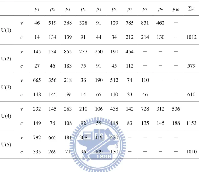
Table 3.1 The Data for Each Project in Example 2 ... 32

Table 3.2 Values, Costs, Efficiencies and Rank for Each Project ... 34

Table 3.3 The Rearrangement of Each Unit’s Project ... 35

Table 3.4 The Decision Variables of the Lower Level for Each Unit’s Project ... 37

Table 4.1 The Inputs and the Outputs for the Proposals of the Divisions ... 55

Table 4.2 The Data of Inputs and Outputs for the Proposals in Example 3 ... 59

Table 4.3 The Results Showing the Input-Output Based Efficiency of Each Proposal ... 62

Table 4.4 The Results Showing the Grey Relational Grade of Each Proposal ... 65

Table 4.5 Implicit Efficiencies for Each Project of Divisions with Proposal Ranking ... 66

Table 4.6 Explicit Efficiencies for Each Project of Divisions with Proposal Ranking ... 67

Table 4.7 The Rearrangement of Each Field’s Projects ... 70

List of Figures

Figure 1.1 Research Flow Chart ... 3

Figure 2.1 A Multiple Hierarchical Structure of Administration ... 5

Figure 2.2 Example of a Rational Reaction Set for a Bilevel Problem ... 8

Figure 2.3 A Geometric Relationship of Interactions of the Leader and the Follower ... 9

Figure 2.4 A Optimal Solution to the Linear BLP ... 12

Figure 2.5 Illustration of BLP Solution by using Definition ... 13

Figure 2.6 Inducible Regions for Versions of the Linear BLPP... 15

Figure 3.1 Diagram of Hierarchical Structure for Resource Allocation ... 25

Figure 3.2 Diagram of the Heuristic Algorithm for BLMF-UC ... 39

Figure 4.1 Diagram of the BLMF-PC Programming System for Budget Allocation ... 46

Figure 4.2 Diagram of the Preprocessing Stage for BLMF-PC ... 73

Chapter 1 Introduction

1.1 Background and Motivations

In the past six, seven decades, many researchers have developed mathematical programming methods in order to solve many decision-making problems. These methods included linear programming (LP), integer linear programming (ILP), multi-objective programming (MOP), and so on. Nevertheless, these methods are not well suited to solving decision-making or management problems in multiple hierarchical structures.

At first, in the late 1970s, the hierarchical structure method was developed from the concept of game theory by decision-making researchers, whom started to pay more attention to multilevel programming (MLP) problems. Then, the MLP method became an even more important tool in dealing with management/hierarchical decision problems. However, development of solution methods in MLP was limited, and the application of MLP was premature at the time. In 1977, Karwan Mark H. and Bialas Wayne F. formed a Decision System Group at SUNY Buffallo to study hierarchical decision problems. In the 1980s, many fundamental results were published in major journals [2-8] by the Decision System Group.

Meanwhile, Shuh-Tzy Hsu [34, 36] and his associates developed the concept that decision makers of each level should optimize one’s own variables/objectives and follow the hierarchy to reach optimum results. Furthermore, by considering a MLP to be a composition of a bilevel programming (BLP), one could reach an optimal solution of MLP. When MLP involves only two levels, it is called a bilevel programming (BLP). In 1994, Yi-Hsin Liu et al, [39, 40] pointed out the geometry of optimal solutions of bilevel linear programming (BLLP) problems. In the late 1990s, the researchers [9, 17, 22] further developed the BLLP model to better fit reality. More recently, Chenggen Shi et al, [11-15, 23] have proposed a series of extended new definition for BLLP theories to deal in terms of deficiency. In fact, the researchers were uninterested in the multiple followers and the applications for the BLP.

The improved model involved one leader and several followers. Bilevel programming with multiple followers is a complicated problem that will be studied in this dissertation. Chapter 2 will discuss the histories and development of the hierarchical optimization and review the mathematical definitions of the continuous and the discrete variables of BLP. Chapter 3 will show the bilevel programming within a multi-follower (BLMF) involving uncooperative condition relationship. Chapter 4 will explain the problems of the partial cooperative relationship under the followers of a BLMF. Finally, a new solution algorithm will be developed to optimize the budget allocation.

1.2 Fields of Study

The research fields of this dissertation include the elements shown below:

(a) A bilevel programming model that includes the upper level and the lower level. (b) A bilevel, multi-follower decision-making system i.e. one single upper level

decision maker (DM) with multiple lower level decision making units (DMUs). (c) The models of the uncooperative and the partial cooperative relationship of a bilevel

involving a multi-follower decision maker.

(d) The limited budget (or resource) allocation models that have been built. (e) The 0/1 knapsack model for an integer programming problem.

(f) The discrete lower level decision variables.

1.3 Objectives of Research

At the present time, none of the existing solution algorithm for the BLP can be treated as the simplex method in the LP. Therefore, an efficient heuristic algorithm is considered in this dissertation. The objectives of this research are listed below:

(a) Develop a bilevel programming model with multiple followers to solve budget allocation problems.

(b) Develop a bilevel budget allocation model to optimize each individual level of objectives.

(c) Discuss the bilevel multiple follower 0/1 programming problems involving uncooperative and partial cooperative variables.

(d) Develop a new GDEA, an improvement of DEA. It is an important procedure of distribution to guarantee the quality of the proposals from the upper level decision maker.

(e) Apply the theory of the grey relationship to obtain the grey relationship grade among all the lower level DMUs in the partial cooperational relationship.

(f) Develop a new heuristic algorithm for the budget allocation solution. It should take advantage of the nature of the bilevel programming problem and offer a feasible solution for this particular model.

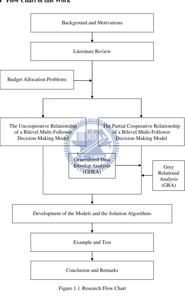
1.4 Flow Chart of this Work

Figure 1.1 Research Flow Chart Background and Motivations

Literature Review

The Uncooperative Relationship of a Bilevel Multi-Follower

Decision-Making Model Budget Allocation Problems

The Partial Cooperative Relationship of a Bilevel Multi-Follower

Decision-Making Model

Example and Test

Conclusion and Remarks

Development of the Models and the Solution Algorithms

Grey Relational Analysis (GRA) Generalized Data Envelop Analysis (GDEA)

Chapter 2 Literatures Review

2.1 History of the Hierarchical Optimization

In 1952, the bilevel programming (BLP) problem was viewed as an uncooperative, two-person game, as introduced by Von Stackelberg. In the basic model, the decision variables are partitioned among the players who seek to optimize their individual pay off functions. Perfect knowledge of information is assumed so that both players know the objective and feasible choices available to the other [26]. (Jonathan F. Bard, 1998)

Two-level planning had been proposed first by Kornai J. and Liptak T. H. in 1965 [27], and they presented a planning task formulated as a single linear programming problem of a maximizing type. This overall central information (OCI) problem is transformed into a two-level problem, in which the ―central problem‖ is the need to create an allocation pattern where the sum of the maximal yields of the ―sector problems‖ will be greatest. The general mode is written as equation (2.1):

(OCI) } min , : { }, max , : { }, 0 , : { }, 0 , : { , min 0 , max b y b y Y y y Y x c x c X x x X y c A y y Y x b Ax x X o y c A y b y x b Ax x c Y y X x                                     (2.1)

be the forms of the primal and dual versions in the OCI problem1. The solution of the two-level program is achieved by a game-theoretical model.

In 1977, the Decision Systems Group began work on a class of n-person decentralized optimization problems that would be known as multilevel programming. Karwan Mark H. and Bialas Wayne F. (1978) [4] released their first report on multilevel programming for the optimization of hierarchical systems. The multilevel optimization techniques parcel out

1 _{The primal variable x is called the OCI program; the dual variable y is the OCI shadow price system. Let X} denotes the set of feasible OCI programs and X* the set of optimal OCI programs, let Y be the set of feasible OCI shadow price systems and Y* the set of optimal OCI shadow price systems.

control over the decision variables of an optimization problem among the decision makers. An important feature is that a planner at one level of the decision hierarchy may have his objective function determined, in part, by variables controlled at other levels.

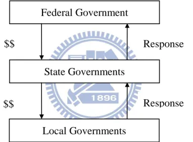
Many decision making problems require compromises among the objectives of several interacting individuals or agencies. Often, these decision makers are arranged within an administrative or hierarchical structure with independent and perhaps conflicting objectives at each level. For example, the policies of the federal government affect the strategies of state officials. Those decisions, in turn, affect the activities of local governments. A multiple hierarchical structure of administrative is illustrated in Fig. 2.1 [2-5] (Bialas and Karwan, 1978-2002).

Figure 2.1 A Multiple Hierarchical Structure of Administration

Source: Bialas Wayne F., ―Multilevel Optimization‖, State University of New York at Buffalo, Industrial Engineering, 2002.

Bialas and Karwan (1984) have noted the following common characteristics of multilevel organizations [7]:

(a) The system has interacting decision-making units within a predominantly hierarchical structure.

(b) Each subordinate/lower level executes its policies after, and in view of, the decisions of the supreme/upper level.

$$

$$

Response

Response

Federal Government

State Governments

Local Governments

(c) Each unit maximizes net benefits independently of other units, but is affected by the actions of other units externally.

(d) The external effect on a decision maker’s problem is reflected in both his objective function and his set of feasible decisions.

When the hierarchical structure is restricted to only two levels, it is categorized as bilevel programming (BLP). The equation of a linear BLP problem is written below:

(BLP) 0 , s.t. max solves where max 2 1 2 2 1 1 2 12 1 11 1 2 22 1 21 2 1 2      x x b x A x A x c x c x x c x c x x x (2.2)

Jonathan F. Bard (1983) [24, 25] developed the bilevel multidivisional programming (BLMP) problem as a model for a decentralized organization. In particular, the model has a hierarchical structure comprised of one leader unit and M follower units. To formulate the problem mathematically, we assume the upper level decision maker wishes to maximize his objective function F and each of the M follower wishes to maximize his own objective function fi. The corporate unit has first choice and selects a strategy x0S0, followed by the M subordinate units that select their strategies xiSi simultaneously. The strategy sets will be given explicit representation:

M i x g x S x g x S0{ 0: 0( 0)0}, i { i: i( i)0}, 1,2,..., . With the BLMP problem defined as equation (2.3):

(BLMP) . ,..., 2 , 1 0 ) , ( s.t. ) , ( max solves ) ..., , ( where 0 ) ( : ) , ( ( max 2 1 0 0 0 0 0 0 M i x x g x x f x x x x x g x x F i i i i i i x M x i     (2.3)

The main feature of the model2 provides pairwise perfect information between leader and follower level payoffs, while permitting each unit to pursue its own goal.

Ben-Ayed O., Boyce D. E., and Blair C. E. (1988) [1] have applied bilevel formulations to the network design problem arising in transportation systems. In the accompanying formulation, a central planner controls investment costs at the system level, while operational costs depend on traffic flows, which are determined by the individual user’s route selection. Assuming users make decisions to maximize their specific utility functions; their choices do not necessarily coincide with the choices that are optimal for the system.

More recently, Chenggen Shi et al, [11-15, 23] have proposed that the leader-level constraint functions in a linear bilevel programming problem are arbitrary in form. Shi, Lu, and Zhang provide not only a new definition for linear BLP theories to deal in terms of deficiency, but they also develop a series of extended approaches to solve the problem.

2.2 Theory of the Bilevel Programming

The bilevel programming (BLP) problem is a special case of multilevel programming (MLP) problems with a structure of two levels. The linear bilevel programming techniques were mainly developed for solving decentralized management problems with decision makers in a hierarchical structure. A decision maker at an upper level is known as the leader, and, at the lower level, is known as the follower [7] (Bialas and Karwan, 1984). Each decision maker (leader or follower) tries to optimize his own objective function with or without considering the objective of the other levels, but the decision of each level affects the objective optimization of the other level. Therefore, the leader may influence the behavior of the follower without completely controlling the follower’s action. At the same time, the leader may be affected by the follower’s behavior [26]. (Bard, 1998)

2 _{Notice that g}i _{is a function not only of x}i _{but each of the other decision variables, call them} i

x . This suggests

i i 

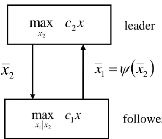
For the special case of n = 2 levels, a bilevel programming problem is a problem with two decision makers. The decision maker 2 is the leader who controls x2 and maximizes

2 22 1 21

2x c x c x

c   , and the decision maker 1 is the follower who controls x1 and maximizes 2

12 1 11

1x c x c x

c   . The leader must announce his choice of x2 before the follower selects x1. Fig. 2.2 represents an example of a rational reaction set for a bilevel problem [2] (Bialas Wayne F., 2002).

Figure 2.2 Example of a Rational Reaction Set for a Bilevel Problem

Source: Bialas Wayne F., ―Multilevel Mathematical Programming: An Introduction‖, State University of New York at Buffalo, 2002.

The leader would like this feasible solution a to be the outcome, but if he chooses this value x at axis x2₂ , then the follower will maximize c₁xc₁₁x₁c₁₂x₂ and respond with this axis x1. x1 

 

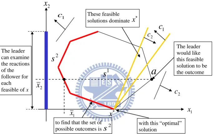
x2 as the follower’s rational response, and it may not be a single value

(see Fig. 2.3 A geometric relationship of interactions of the leader and the follower).

1

s

1

c

2

c

1

x

a

2

x

1

x

2

c

1

c



x

2

s

with this ―optimal‖ solution The leader would like this feasible solution to be the outcome These feasible solutions dominate

x



to find that the set of possible outcomes is

s

2 2

x

The leader can examine the reactions of the follower for each feasible of x

Figure 2.3 A Geometric Relationship of Interactions of the Leader and the Follower

For a given x2 from the leader, the follower solves in (2.4)

(Follower) 0 s.t. max 1 2 2 1 1 2 12 1 11 2 1     x x A b x A x c x c x x (2.4)

the leader can examine the reactions of the follower for each feasible choice of x2 and find that the set of possible outcomes is S2. The leader’s problem is actually to find in (2.5)

(Leader) solves where , ) , ( s.t. max 1 2 2 1 2 22 1 21 2 x S x x x c x c x   (2.5) ) , ( ₁ ₂ _ x x

x with this optimal solution in the bilevel programming problem. Even in the linear case, the bilevel programming problem is a non-convex optimization problem. The solution represents the stable outcome of the bilevel decision process that need not be Pareto optimal3.

There is an important concept regarding a model with two (or more) objectives. Usually a model with two objectives is either a bilevel (hierarchical environment) or bi-objective (optimize two objectives simultaneously), and these two models are different.

3

Given a set of alternative allocations of goods or income for a set of individuals, a change from one allocation to another that can make at least one individual better off without making any other individual worse off is called a Pareto improvement. An allocation is Pareto efficient or Pareto optimal when no further Pareto improvements can be made. The Pareto optimum is a state of allocating the resources where it is no longer

x

c

x2 2

max

x

c

x x_{1 2} 1

max

leader

follower

 

₂ 1

x

x





2

x

2.3 The Variables of the Bilevel Programming

2.3.1 Continuous Variables

The hierarchical structure of the BLP problem imposes a strict order on the selection of the decision variables each planner controls. That is, the follower decision level executes its policies after, and in view of, the decision of the leader level, and the leader level optimizes its objective independently over the reactions from the follower level [39, 40]. (Yi-Hsin Liu, Stephen M. Hart and Thomas H. Spencer, 1994-1995)

Let the vectors _a,c,x_Rn1_{, b,d,y}_Rn2_{, and u}_Rm_{. Further, let A and B be two}

matrices with size m×n1 and m×n2, respectively. Given this, the BLP problem is the equation (2.6): (BLP I)

 

 

S y x dy cx y x f y by ax y x F y x      ) , ( s.t. , max solves where , max (2.6)

The constraint set S {(x,y):AxByu,(x,y0)} is assumed to be a bounded, nonempty subset of _Rn1n2_.

Since S is assumed bounded and nonempty, for each x , the follower planner’s problem,

 

0 , s.t. , max     y x A u By dy y x f y

has an optimal solution. The set of all optimal solutions with respect to this x is called the feasible reaction set for the follower planner and is denoted Y

 

x . The leader planner’s feasible region, also referred to as the set of all rational reactions of f over S, is defined as

)} ( , ) , ( : ) , {( ) (S  x y x y S yY x  .

a point (x,y)(S) such that axbyaxby for all (x,y)(S) is called an optimal solution of the BLP.

The geometric properties of BLP problem have been well explored, and the pertinent ones are presented below:

(a) (S) is a connected subset of S.

(b) If there is an optimal solution to the BLP problem, then there is an extreme point of

) (S

 that is an optimal solution of the BLP problem, and hence there is an extreme point of S that is an optimal solution of the BLP problem.

The following theorem provides a geometric characterization of an optimal solution of a BLP problem.

Theorem 1. If an optimal solution of the leader objective function over S is in (S), then it is an optimal solution to the BLP problem.

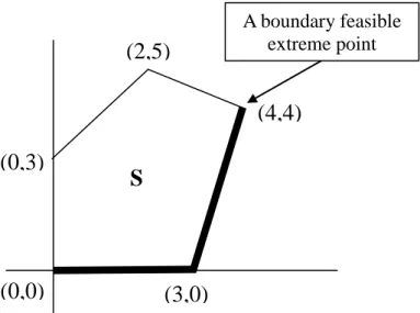
Theorem 2. If there exists an optimal solution of the leader objective function over S not in (S), there exists a boundary feasible extreme point that optimizes the BLP problem. Example 1: 0 , 0 12 4 12 2 3 s.t. max solves where 3 max            y x y x y x y x y y y x y x

The illustration of the method is presented in Fig. 2.4. It is easy to see that (S) is the set of points on line segments connecting (0, 0), (3, 0), and (4, 4), while the optimal solution of this BLP problem is the point (4, 4), which is a boundary feasible extreme point.

Figure 2.4 A Optimal Solution to the Linear BLP

Corresponding to the equation (2.6) and example 1, Bard (1998) [26] gave the following basic definition for a linear BLP solution:

(a) Constraint region of the BLP problem:

 







, :  ,  ,   , , 0



 x y x X y Y Ax By u x y

S .

(b) Feasible set for the follower for each fixed xX:



y Y By u Ax



x

S( )  :  

(c) Projection of S onto the leader’s decision space:



x X y Y By u Ax



X

S( )  :  ,  

(d) Follower’s rational reaction set for xS( X):











( ,ˆ):ˆ ( )





( ): ( , ) ( ,ˆ), ˆ ( )



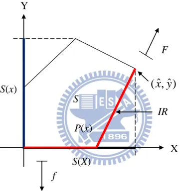
max arg where ) ( ˆ : ) ˆ , ( max arg : ) ( x S y y x f y x f x S y x S y y x f x S y y x f y Y y x P         

(e) Inducible region:



(x,y):(x,y) S,y P(x)



IR  

The rational reaction set P(x) defines the response while the inducible region IR represents the set over which the leader may optimize his objective. Thus, in teams of the above notations, the linear BLP problem can be written as:



F(x,y):(x,y)IR



max

(0,0)

_(3,0)

(0,3)

(4,4)

(2,5)

A boundary feasible extreme point

S

To ensure that Fig. 2.5 has an optimal solution, Bard (1998) [26] gave the following assumption:

(a) S is nonempty and compact.

(b) For all decisions taken by the leader, the follower has some room to respond, i.e.,   ) (x P . (c) P(x) is a point-to-point map.

Figure 2.5 Illustration of BLP Solution by using Definition

2.3.2 Discrete Variables

In many optimization problems, a subset of the variables is restricted to only take on discrete value. This can complicate the problem. To specify the model, let x1 be an n1-dimensional vector of continuous variables and x2 be an n2-dimensional vector of discrete variable, where x=(x1,x2) and n=n1+n2. Similarly, define y1 as an m1-dimensional vector of continuous variables and y2 as an m2-dimensional vector of discrete variable, where y=(y1,y2) and m=m +m . This leads to

Y

X

S

S(x)

S(X)

IR

f

F

P(x)

)

ˆ

,

ˆ

(

x

y

(BLP II) integer 0 , 0 s.t. ) ( min integer 0 , 0 s.t. ) , ( min 2 2 2 2 22 1 21 2 22 1 21 2 22 1 21 1 1 1 2 12 1 11 2 12 1 11 2 12 1 11 2 12 1 11                   y x b y B y B x A x A y d y d y f y x b y B y B x A x A y d y d x c x c y x F y x (2.7)

where all vectors and matrices are of the conformal dimension, and the linear terms in x have been omitted from the follower’s objective in function (2.7) [26] (Bard, 1998).

Note that it may be desirable to explicit include additional restrictions, such as upper and lower bounds, on the variables. In this case, let xX {x:l1_j x_j u1_j, j1,2,...,n} and

} ,..., 2 , 1 , : {y l2 y u2 j m Y y  _j  _j  _j  .

Bard has investigated the properties of the zero-one linear BLP problem when some or all variables are restricted to binary values. Based on the specific instances of (2.7), it will be convenient to consider the problem in the form of (2.6) without reference to which variables are continuous and which are discrete; i.e.,

integer 0 , 0 subject to ) , ( min solves where subject to ) , ( min 2 2 2 2 1 1 1 1 1            y x b y B x A y d y x f y b y B x A y d x c y x F Y y K x (2.8) where c₁Rn,d₁,d₂Rm,b₁Rp,b₂Rq,A₁Rpn,B₁Rpm, A₂Rqn,B₂Rqm, m n R Y R X and  .

In addition to the definition in section 2.3.1, let S_L(y){xX :A₂xb₂ B_2y}, for all values of yY, and SU(y){(x,y):A1xB1y b1}.

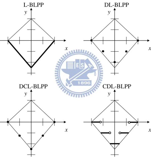
For each xX, it will be assumed that the optimal solution of the lower level problem is unique. Along with the linear bilevel programming problem (L-BLPP) where X=Rn and Y=Rm, there are three models as shown below:

(a) Discrete linear bilevel programming (DL-BLP) problem, where4 X=Bn and Y=Bm;

(b) Discrete-continuous linear bilevel (DCL-BLP) problem, where X=Bn and Y=Rm; and (c) Continuous-discrete linear bilevel (CDL-BLP) problem, where X=Rn and Y=Bm.

Figure 2.6 depicts the inducible regions associated with the four problems.

Figure 2.6 Inducible Regions for Versions of the Linear BLPP

Source: Bard Jonathan F., ―Practical Bilevel Optimization: Algorithms and Applications‖, Kluwer Academic Publishers, Netherlands, pp.235, 1998.

x

y

L-BLPP

x

y

DL-BLPP

x

y

DCL-BLPP

x

y

CDL-BLPP

Corresponding to Fig. 2.6, Bard (1998) [26] presented some properties and theorems as shown below: Property 1: If SU Rn m   , then IR is nonempty if S . If SU Rn m   , then IR is nonempty if there exists a xX such that (x,y)S_U.

Property 2: The inducible regions of DCL-BLPP and DL-BLPP are included in the inducible regions of L-BLPP and CDL-BLPP, respectively.

Property 3: For the L-BLPP, let S be a bounded set, i.e., a polytope. If n m U R

S   , then

L-BLPP, DL-BLPP, and DCL-BLPP have an optimal solution if S. If

m n U R

S   , then L-BLPP, DL-BLPP, and DCL-BLPP have an optimal solution if exists a xX such that (x,y)S_U.

Theorem: Let SU Rn m



 , S and suppose there exists an optimal solution (x*,y*) to CDL-BLLP. Then (x*,y*) is a boundary (bd) point of S.

Algorithms designed to solve integer programs generally rely on some separation, relaxation, and understanding to construct ever-tighter bounds on the solution.

2.4 Summaries

The bilevel programming problem can be viewed as an uncooperative, two-person game; in this model, the players seek to optimize their individual pay off functions. Since 1977, Karwan and Bialas formed a Decision System Group to study hierarchical decision problems. Many fundamental results were published in major journals by this group. An important feature is that a planner at one level of the decision hierarchy may have his objective function determined, in part, by variables controlled at other levels.

The BLP problem is a special case of the multilevel programming problem with a two-level structure. The BLP problem imposes a strict order on the selection of the decision variables each planner controls. That is, the follower decision level executes its policies after, and in view of, the decision of the leader level, and the leader level optimizes its objective independently over the reactions from the follower level.

The BLP problems that include continuous and discrete variables are examined in this chapter. The principal concepts and a formal definition of the continuous variables are presented by Yi-Hsin Liu. There are two geometric properties of the problem as shown:

(a) (S) is a connected subset of S.

(b) If there is an optimal solution to the BLP problem, then there is an extreme point of

) (S

 that is an optimal solution of the BLP problem, and hence there is an extreme point of S that is an optimal solution of the BLP problem.

In many optimization problems, a subset of the variables is restricted to only take on discrete value. Bard has investigated the properties of the zero-one linear BLP problem when some or all variables are restricted to binary values. There are three models shown below:

(a) Discrete linear bilevel programming (DL-BLP) problem. (b) Discrete-continuous linear bilevel (DCL-BLP) problem. (c) Continuous-discrete linear bilevel (CDL-BLP) problem.

The common methods used to solve a linear bilevel programming problem and are related to the continuous variables are the kth-Best algorithm and Kuhn-Tucker approach. In addition, another method related to the discrete variable is Branch and Bound notation. All of the detail algorithms can be found in Bard’s work (1998) [26] ―Practical Bilevel Optimization: Algorithms and Applications‖.

Chapter 3 The Uncooperative Relationship of a Bilevel

Multi-Follower Decision-Making Model

3.1 Introduction

A bilevel programming (BLP) problem is a special case of the multilevel programming (MLP) problem with a structure of two levels. The bilevel programming techniques are mainly developed for solving decentralized management problems with decision makers in a hierarchical organization (see Chapter 2). A decision maker at an upper level is known as the leader, and at the lower level is the follower [7] (Bialas Wayne F. and Karwan Mark H., 1984). Each decision maker (DM) (leader or follower) optimizes his/her own objective function with or without considering the objective of the other level, but the decision of each level affects the optimization of the other level. Therefore, the leader may influence the behavior of the follower without completely controlling the follower’s action. At the same time, the leader may be affected by the follower’s behavior [26] (Jonathan F. Bard, 1998).

Usually, in a real world situation, there is more than one follower in the lower level; this type of the hierarchical structure is called a bilevel multi-follower (BLMF) decision-making model. However, the different relationships among these followers might force the leader to use multiple different processes in deriving an optimal solution for leader decision making. Therefore, the leader’s decision will be affected not only by the reactions of these followers, but also by the relationships among these followers. In general, there are three kinds of relationships among the followers; these relationships are determined by how decision variables [23] (Jie Lu, et al.) are shared among the followers. These scenarios are as follows:

(a) The cooperative situation where the followers totally share the decision variables in their objectives and constraints.

(b) The uncooperative situation where there is no sharing of decision variables among the followers.

(c) The partial cooperative situation where the followers partially share decision variables in their objectives and/or constraints.

If the cooperative situation among various followers in case (a) takes place, then the problem is equivalent to a situation where all units of the lower level act as a single unit with only one objective function. In such cases, the linear BLMF programming problem is reduced to a linear BLP one [34] (Shuh-Tzy Hsu, An-Der Huang and Ue-Pyng Wen, 1993).

The case (b) above will be discussed carefully in this chapter. The most problematic situation for a hierarchical structure of linear bilevel multi-follower decision-making is the uncooperative situation where there is no sharing of decision variables among the followers [34, 23] (e.g., Hsu S. T., Hung A. D., and Wen U. P., 1993; Lu J., Shi C., and Zhang G., 2006). This situation can be formulated as follows:

For xX Rn_,y_iY_i Rmi_,Y ₍Y_,Y _,...,Y_K)T_,F_:XY _...Y_K R1_,f_i:XY_i 

1 2

1

R1 and i1,2,...,K, a linear BLMF decision problem in which K(2) followers are involved and there is no shared decision variable, objective functions, and constraint function among them is defined as follows:





       K s s s K s s s k X x b y B Ax y d cx y y x F 1 1 1 s.t. ) ,..., , ( min (3.1)

where yi (i1,2,...,K), for each value of x, is the solution of the lower level problem:

i i i i i i i i i b y C x A y e x c y x f     s.t. ) , ( max (3.2) where cRn,c_iRn,d_iRmi,e_iRmi, bRp,b_iRqi,ARpn,BRpm,B_iRpmi, K i R C R A qi mi i n i q i ,  , 1,2,...   .

According to the definitions above, there are four characteristics of the uncooperative relationship of a linear BLMF (BLMF-UC) decision-making problem as follows:

(a) A bilevel decision-making system with one single upper level DMU and multiple lower level DMUs.

(b) The upper level DM controls a set of variables, while each lower level DMU controls one’s own decision variables.

(c) Each lower level DM’s decision variables are independent, i.e. uncooperative.

(d) Each lower level DM optimizes its own objective, hence, the lower level solves multiple objective programming problems.

Based on the definitions and characteristics stated above, a budget allocation model is constructed to discuss the nature of BLMF-UC. Since the structure of the budget allocation problem is hierarchal with multi-followers, this problem not only involves two decision-making levels, but it also is an uncooperative situation where there is no sharing of decision variables among the followers.

Generally speaking, the structure of the budget allocation problem studied in this work is a bilevel programming problem with 0/1 variables, which is difficult to solve. Therefore, the purposes of this chapter are to formulate a new model and to propose an efficient heuristic algorithm for this problem.

3.2 Budget allocation problems

An organization’s management requires information about the resources available to achieve the organization’s purpose. Resources are acquired, allocated, and manipulated under the manager’s control. The organization’s purpose is sometimes stated as its vision or goal. The vision or goal is attained through the achievement of multiple, numerous, and often competing objectives [31] (Richard O. Mason and Swanson E. Burton, 1979).

There are a variety of ways to achieve a systematic and rational allocation of resources that will provide a competitive advantage to an organization. The methodology discussed below is quite flexible and can be adapted to a wide variety of situations and constraints. The methodology consists of the following steps [19] (Ernest H. Forman and Mary Ann Selly, 2001):

Step 1: Identify/design alternatives

Expertise in the art and science of identifying and/or designing alternatives lies in the domain of the decision makers, who have many years of study and experience with which to act on this task. The goal here is to help them attain better measurements and syntheses in order to better capitalize on their knowledge and experience.

Step 2: Identify and structure the organization’s goals and objectives

The main message is that decisions must be made on the basis of achievement of objectives with resource allocation decisions. And so the entire enterprise’s goals and objectives must be addressed. The executives understand these goals and objectives and can best make judgments about the relative importance of the main organizational objectives and, possibly, the sub-objectives.

Step 3: Prioritize the objectives and sub-objectives

The relative importance of the objectives and sub-objectives must be established in order to make a rational allocation of resources. The prioritization of the organization’s objectives during the resource allocation process will lead to another important advantage—in the top management’s quest for excellence, one will be able to respond to shifts in direction brought about by changes in the environment and competitive forces.

Step 4: Measure alternative’s contribution

Having prioritized the organization’s objectives and sub-objectives, the next step is to evaluate how much each proposed activity (or each possible level of funding for each activity) would contribute to each level’s objectives.

Step 5: Find the best combination of alternatives

After prioritizing the organization’s objectives and sub-objectives and rating the contribution of the competing activities, the lowest level objectives, etc., we have ratio scale measures of the relative contribution of each alternative combination to the organization’s overall objectives.

Otherwise, in applied mathematics, the resource allocation (RA) problem is an optimization problem with a single constraint. Given a fixed amount of the resource B (this is the constraint), DM is asked to determine its allocation to n activities in such a way that the objective function under consideration is optimized. The simple structure of the resource allocation problem discussed is generally formulated as (3.3) [35] (Toshihide Ibaraki and Naoki Katoh, 1988): (RA) . ,..., 2 , 1 , 0 subject to ) ,..., , ( maximize 1 2 1 n j x B x x x x f j n j j n   



 (3.3)

That is, given one type of resource whose total amount is equal to B, DM wants to allocate it to n activities so that the objective value f(x₁,x₂,...,x_n) becomes as large as possible. The objective value may be interpreted as the profit or reward, and it is natural to maximize f. DM will sometimes considers minimization problems such as the cost, time, or loss.

In general, limited resources must be allocated among several activities, and linear programming often solves resource allocation problems. To use linear programming to allocate resources, Wayne L. Winston in 1991 [37] made three vital assumptions:

(a) The amount of a resource assigned to an activity may be any non-negative number. (b) The benefit obtained from each activity is proportional to the amount of the

resource assigned to the activity.

(c) The benefit obtained from more than one activity is the sum of the benefits obtained from the individual activities.

Wayne L. Winston (1991) [37] had considered a generalized resource allocation (GRA) problem. Suppose that the organization has B units of resource available and n activities to which the resource can be allocated. If activity j is implemented at a level xj (assume xj must be a nonnegative integer), then gj(xj) units of the resource are used by activity j, and a

maximizes total benefit that is subject to the limited resource available may be written as the following equation (3.4): (GRA) integer : ,..., 2 , 1 ; 0 ) ( . s.t ) ( max 1 1 j j j n j j j n j j x n j x B x g x v   





  (3.4)

The other important and very common algorism uses 0-1 variable to represent binary choice. Consider an event that may or may not occur and suppose that it is part of the problem in deciding between these two possibilities. To model such a binary, variable x is used and let

     occur not do event the if 0 occurs event the if 1 x

Suppose there are n projects. The jth project (j1,2,...,n) has a cost cj and a value of j

v . Each project is either done or not done; that is, it is not possible to do a fraction of any of the projects. Also, there is a budget of B available to fund the projects. The problem of choosing a subset of the projects to maximize the sum of the values while not exceeding the budget constraint is the 0-1-knapsack (KP) problem. It is written as the following equation (3.4) (George L., Nemhauser, Laurence A. and Wolsey, 1988) [21]:

(KP-RA) } 1 , 0 { s.t. max 1 1  





  x B x c x v n j j j n j j j (3.5)

This problem is called the knapsack problem because of the analogy to the hiker’s problem of deciding what should be put in a knapsack given a weight limitation on how much can be carried.

According to the methodology of resource allocation mentioned above, the organization makes resource decisions in a rational way in order to achieve its vision or goals. The organization must do the following:

(a) Identify/design alternatives.

(b) Identify and structure the organization’s objectives. (c) Prioritize the objectives and sub-objectives.

(d) Measure alternatives’ contribution. (e) Find the best combination of alternatives.

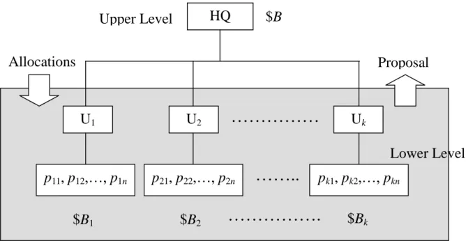
Suppose the headquarters (HQ) of an organization has a budget $B available and the budget will be distributed to its follower units (Ui). The problem of determining the allocation of resources is how one should maximize total contribution (or value) that is subject to the limited resource available. That is, a HQ should refer to the five principles above before a decision is made to allocate resources. The operating procedure includes:

(a) The HQ (upper level) draws out concrete resource allocation rules and measures from the organization’s visions or goals.

(b) Based on these rules and measures, the lower level evaluates its sub-objectives and submits its resource requirement proposal (pij). Each proposal must contain cost (cij) and anticipated value (vij).

(c) The HQ examines proposals before finally issuing the optimal allocation of its limited resources.

Based on the procedure above, a two-stage reviewing process is used. Stage 1, the proposals are reviewed by a committee to ensure the significance of the proposal for the organization’s visions or goals. In this stage, some proposals are disqualified. Stage 2, the committee decides whether the qualified proposals are to be funded or not and how much each should receive in funds. The funded proposals must maximize contribution within a limited budget. Fig. 3.1 is a diagram showing the hierarchical structure for resource allocation.

Figure 3.1 Diagram of Hierarchical Structure for Resource Allocation Source: Study

The problem is the 0-1-knapsack problem. Basically, it may be written as an equation (3.6) in order to maximize the total value that is subjected to the limited resource available and to achieve an organization’s objective.

} 1 , 0 { ,..., 2 , 1 , s.t. ,..., 2 , 1 , max 1 1 1     







   ij k i i n j i ij ij n j ij ij x B B k i B x c k i x v (3.6)

vij: The anticipated value from the jth project of the ith unit. cij: Cost required in the jth project of the ith unit.

xij: Decision variable of the jth project of the ith unit.

$B

1

HQ

Allocations

Proposal

Lower Level

U

1

U

2

U

k

p

11

, p

12

,…, p

1n

p

21

, p

22

,…, p

2n

p

k1

, p

k2

,…, p

kn

$B

2

……….

$B

k

……..

………

$B

Upper Level

3.3 Model Development

These budget allocation problems can be modeled as a 0/1 integer program; however, computation efficiency is a concern. The particular problems studied in this research belong to the problem of NP hard5, which suggests an efficient heuristic algorithm is necessary. This problem is formulated as a bilevel multi-follower programming involving the uncooperative decision variables (BLMF-UC), where the lower level decision maker’s problem is a mathematical programming problem with independent, multiple objectives; then, the upper level DM, the leader, must solve the optimization problem over the lower level decision maker’s rational reaction set.

The HQ of this particular company has funds of $B for the distribution to each of the k divisions under its supervision. The distribution process follows the rules below:

(a) Each division (follower or unit) summits proposal(s) to apply for funding.

(b) Each proposal (P) clearly and correctly states the work project, the cost (C) requirements to complete the project, and the value (V) of the project accomplishments.

(c) At least one proposal from each division must be funded.

(d) The overall efficiency/value is maximized (i.e. the subobjective of each lower level decision maker).

(e) The differences in the levels of satisfaction (as defined below) among the divisions are minimized (i.e. the objective of the upper level decision maker).

Note: Statement 3 above is necessary, otherwise the funding distribution process will be impossible to achieve.

5 _{In computational complexity theory, NP-hard (Non-deterministic Polynomial-time hard) refers to the class of} decision problems that contains all problems H such that for all decision problems L in NP there is a polynomial-time many-one reduction to H. Informally this class can be described as containing the decision problems that are at least as hard as any problem in NP. This intuition is supported by the fact that if we can find an algorithm A that solves one of these problems H in polynomial time then we can construct a polynomial time algorithm for every problem in NP by first executing the reduction from this problem to H and then executing the algorithm A.

In order to distribute the funds according to the rules above, a model is developed and is shown below. First, some basic definitions are given, and notations are introduced.

In a bilevel budget allocation programming problem with the uncooperative relationship, the goal of the upper level DM is to seek the most rational way of distributing the budget to each follower division simultaneously. The leader wants to balance the growth among all individual divisions and promote the strength of the entire organization within the industry as well. In order to do so, the objectives are to minimize the level of satisfaction among the individual divisions upon their funding approvals. Therefore, the upper level DM’s problem is [P1]:

[P1] to minimize the level of satisfaction among the funded individual divisions, so that abalanced resource is allocated to lower units.

Under the resource allocation policy of the upper level DM, the lower level DM will pursue the largest value of each individual division in order to maximize the total value of the organization. Hence, this distribution is reasonable for lower level DMs.

In other words, one should understand the strengths and weaknesses among the divisions to make the rational decision. The rational decision of the lower level DM is to maximize the total value of his/her division. Therefore, the lower level DM’s problem is [P2]:

[P2] to maximize the total value of each division while the costs stay within the funding limits.

In this decision-making problem, [P1] and [P2] are two closely related models; they are not separable. There is a natural hierarchical relationship tie between [P1] and [P2]. More precisely, the upper level DM selects the policy of resource allocation, and the lower level DM gives systematic reactions under this policy. The upper level DM then makes a rational decision after reviewing the systematic reactions of lower level DM. The relationship of [P1] and [P2] can be considered as the hierarchical programming problem [P]:

[P] to choose certain proposals to maximize the value of each division and to minimize the differences of the level of satisfaction among the divisions funded, simultaneously, the costs stay within the funding limits.

More precisely, the above is restated as:

[P] Minimize the difference of level of satisfaction among the division funded

where the chosen factors (proposals) will minimize the level of satisfaction and solve the problem

Maximize the value of each division

Subject to the costs stay within the funding limits

The hierarchical programming problem [P] above is a case in which the lower level decision variables are uncooperative for this type of bilevel multi-follower/multi-objective programming; it is the uncooperative relationship (BLMF-UC) problem. The mathematical model of a BLMF-UC problem is formulated as follows:

Let U(i):i1,2,,k be k divisions/units of funds to be distributed, and let

: ) , ( { ) (i p i j

P  j1,2,,n} be the collection of n proposals submitted by division i to request funding. Without loss of generality, we can assume that every division submits n proposals, and each proposal has a cost, c( ji, ), which denotes the cost required to accomplish p( ji, ). And v( ji, ) denotes the value obtained when p( ji, ) is accomplished.

The efficiency of project j in the division i is the ratio of the value to the requested funding. i.e. ) , ( ) , ( ) , ( j i c j i v j i e  (3.7)

Otherwise, the level of satisfaction of division i is the ratio of the total funded amount to the total requested amount.

i.e.





   _n j n j j i c j i y j i c i L 1 1 ) , ( ) , ( ) , ( ) ( (3.8)

Thus, the model of BLMF-UC for this problem aims to minimize any difference in the satisfaction levels among the divisions, while the total efficiency obtained from the funded proposal is maximized. In addition, the conditions below must be satisfied:

x is the variable of the leader, DM, while y(i) is a vector valued variable of each lower level DM. The decision variable y( ji, ) is defined as below.

     otherwise 0 funded is ) , ( if 1 ) , ( j i p j i y

In each division, the total cost of a funded proposal cannot exceed the dollar amount allotted to this division. Moreover, the total of the allotted amount for all divisions cannot exceed $B, which is the available funding for distribution.

The mathematical model of BLMF-UC is then formulated in (3.9) and is shown as follows: (BLMF-UC) n j k i i B j i y B i B k i j i y k i i B j i y j i c k i j i y j i v j i y k m i m L i L x x k i n j n j n j ,... 2 , 1 ,..., 2 , 1 , 0 ) ( } 1 , 0 { ) , ( ) ( ,..., 2 , 1 , 1 ) , ( ,... 2 , 1 , ) ( ) , ( ) , ( s.t. ,..., 2 , 1 ), , ( ) , ( max solves ) , ( where , 1 ), ( ) ( s.t. min 1 1 1 1                            (3.9)

Note: xL(i)L(m), 1i,mk implies x is greater than the difference between the maximum L(i) and minimum L(i) among all i1,2,,k.