無線感測網路下適用於橢圓曲線加密機制之快速窗口純量乘法演算法

國

立

交

通

大

學

無線感測網路下適用於橢圓曲線加密機制

之快速窗口純量乘法演算法

A Fast Window-based Scalar Multiplication Algorithm for Elliptic

Curve Cryptography in Wireless Sensor Networks

研 究 生：葉宏男

無線感測網路下適用於橢圓曲線加密機制

之快速窗口純量乘法演算法

A Fast Window-based Scalar Multiplication Algorithm for

Elliptic Curve Cryptography in Wireless Sensor Networks

研 究 生：葉宏男 Student：Hung-Nan Ye

指導教授：王國禎 Advisor：Kuochen Wang

國 立 交 通 大 學

資 訊 科 學 與 工 程 研 究 所

碩 士 論 文

Submitted to Institutes of Computer Science and Engineering Department of Computer Science

National Chiao Tung University in Partial Fulfillment of the Requirements

for the Degree of Master

in Computer Sciencmae June 2011

無線感測網路下適用於橢圓曲線加密機制

之快速窗口純量乘法演算法

學生：葉宏男 指導教授：王國禎 博士

國立交通大學資訊科學與工程研究所

摘 要

最近幾年來，由於無線感測網路廣泛的應用在軍事、環境監控、健康和

居家照顧上，使得其在安全性方面變得越來越重要。加密機制是一個提供

安全服務的基本技術。因為感測節點的資源有限，所以在執行加密時必須

減少計算、通信和記憶體的負載。橢圓曲線加密機制和其他的加密機制比

較，其在通訊、計算和記憶體的使用需求上比較少。此外，在相同的安全

層次上，橢圓曲線加密機制只需要160位元的金鑰長度，而RSA加密演算法

則需要1024位元的金鑰長度，所以橢圓曲線加密機制非常適合用在無線感

測網路上。然而，橢圓曲線加密機制的金鑰產生包含許多的純量乘法，使

得其應用在感測節點上仍需要耗費許多的執行時間。在本論文中，我們提

出一個在無線感測網路下適用於橢圓曲線加密機制之快速窗口純量乘法演

算法(EW-MOF)。這個方法結合了相互交替型式和改良式窗口方法，它不

只可以減少預先計算的時間和記憶體的使用，而且還可以減少每一個感測

節點包含預先計算時間的平均時間。我們的分析結果顯示，EW-MOF所需

要預先計算點的數目比1的補數演算法還要少，因此它非常適合用在無線感

測網路上。此外，模擬結果顯示，我們提出的EW-MOF在不同的質數域下，

包含預先計算時間的橢圓曲線加密機制，其平均金鑰產生時間比傳統1的補

數演算法還要快24.69%。總之，在節省能源和金鑰產生時間方面，EW-MOF

比1的補數演算法更適用在無線感測網路上。

關鍵詞：橢圓曲線密碼學、相互交替型式、1的補數、純量乘法、窗口方法。

A Fast Window-based Scalar Multiplication

Algorithm for Elliptic Curve Cryptography in

Wireless Sensor Networks

Student：Hung-Nan Ye Advisor：Dr. Kuochen Wang

Department of Computer Science National Chiao Tung University

Abstract

In recent years, the security of wireless sensor networks (WSNs) has become more and more important due to extensive applications of WSNs in the areas of military, environmental monitoring, health and homecare. Cryptography is a basic technique to provide security services for WSNs. Owing to the limitation of resources in sensor nodes, the computation, communication, and memory overheads introduced by performing cryptography must be minimized. Elliptic curve cryptography (ECC) compared to other cryptosystems requires less communication, computation, and memory usages. Hence, ECC is suitable for wireless sensor network security because ECC only requires 160 bits length of keys to achieve the same level of security as RSA using 1024 bits length of keys. However, the key generations in ECC, which involve with a large number of scalar multiplications, is still time consuming when applied to sensor nodes. In this paper, we propose an enhanced window-based mutual opposite form (EW-MOF) for scalar multiplication with ECC in WSNs. The proposed EW-MOF combines MOF with an enhanced window method that can reduce not only pre-computation time and memory usage, but also average key generation time including pre-computation time in each sensor node. Our analysis has shown that the proposed

EW-MOF requires a smaller number of essential pre-computed points than the one’s complement and therefore it is very suitable for WSNs. Simulation results show that the proposed EW-MOF is 24.69% faster than the one’s complement method, which is a classical method, in the average key generation time of ECC including pre-computation time under different field sizes. In summary, the proposed EW-MOF is more feasible than the one’s complement for wireless sensor networks in terms of key generation time and power saving.

Keywords: Elliptic curve cryptography, mutual opposite form, one’s complement, scalar

Acknowledgements

Many people have helped me with this thesis. I am in debt of gratitude to my thesis advisor, Dr. Kuochen Wang, for his intensive advice and guidance. I would also like to show my appreciation for all the classmates in the Mobile Computing and Broadband Networking

Laboratory for their invaluable assistance and inspirations. The support by the National

Science Council under Grants NSC99-2218-E-009-002 is also gratefully acknowledged. Finally, I thank my father, my mother and my friends for their endless love and support.

Contents

Abstract (in Chinese)……….………...i

Abstract ... iii

Contents ... vi

List of Figures ... viii

List of Tables ... ix Chapter 1 Introduction ... 1 1.1 Motivation ... 1 1.2 Cryptography ... 2 1.3 Problem statement ... 2 1.4 Thesis organization ... 3 Chapter 2 Background ... 4

2.1 Elliptic curve cryptography overview ... 4

2.2 Elliptic curve Diffie-Hellman protocol ... 5

Chapter 3 Related Work ... 7

3.1 Binary method [3] ... 7

3.2 Non-adjacent form [9]... 7

3.3 Mutual opposite form [10] ... 8

3.4 Complementary recoding [12] ... 8

Chapter 4 Proposed EW-MOF Algorithm ... 11

4.1 Why use MOF for scalar multiplication ... 11

4.1.1 NAF ... 12

4.1.2 MOF ... 12

4.1.3 Complementary recording ... 13

4.2 Design of the proposed enhanced window method ... 15

4.3 Design the proposed EW-MOF algorithm ... 18

Chapter 5 Performance Evaluation and Discussion ... 25

5.1 Simulation environment setup ... 25

5.2 Comparison between the proposed EW-MOF and one’s complement ... 25

5.3 Discussion ... 29

Chapter 6 Conclusion ... 30

6.1 Concluding remarks ... 30

6.2 Future work ... 31

List of Figures

Figure 1. Sensor nodes randomly deployed in a sensor field. ... 1

Figure 2. Three addition cases in an elliptic curve. ... 5

Figure 3. Elliptic curve Diffie-Hellman protocol. ... 6

Figure 4. An illustration of how to derive pre-computed points for w = 5 in MOF. ... 13

Figure 5. Comparison of the number of pre-computed points under different window sizes among NAF, MOF, complementary recoding. ... 14

Figure 6. Enhanced window method for deriving essential pre-computed points. ... 15

Figure 7. Comparison of the number of essential pre-computed points under different window sizes in MOF. ... 17

Figure 8. Selection of the best window size under N (assuming 100) times of key generations. ... 18

Figure 9. Flowchart of selecting an elliptic curve and a base point for ECC in WSNs. ... 22

Figure 10. Flowchart of the public key generation process for a sensor node. ... 23

Figure 11. Average key generation time excluding pre-computation time under different field sizes. ... 26

Figure 12. Average key generation time including pre-computation time under different field sizes. ... 27

Figure 13. Average key generation time, excluding pre-computation time, under different window sizes. ... 28

Figure 14. Average key generation time, including pre-computation time, under different window sizes. ... 29

List of Tables

Table 1. Comparison of key lengths in different security levels [7]. ... 4 Table 2. Comparison of three existing scalar multiplication algorithms. ... 9 Table 3. Comparison of the numbers of pre-computed points and doubling and addition

operations under different window sizes. ... 10 Table 4. Best selection of S under different window sizes. ... 17

Chapter 1

Introduction

1.1 Motivation

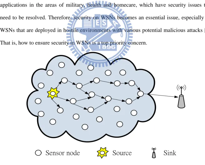
Wireless sensor networks (WSNs) are formed by a large number of sensor nodes which have features of small size, low cost, low power consumption, and limited computation and communication capabilities. Each sensor node is used to collect data from the environment and to transmit data back to the sink, as shown in Figure 1. In recent years, WSNs have wide applications in the areas of military, health and homecare, which have security issues that need to be resolved. Therefore, security on WSNs becomes an essential issue, especially for WSNs that are deployed in hostile environments with various potential malicious attacks [1]. That is, how to ensure security in WSNs is a top priority concern.

Source

Sensor node

Sink

1.2 Cryptography

Generally speaking, network security focuses on three major issues: authentication, confidentiality and integrity. Cryptography is a basic technique to provide security services to address the above issues in a network [2]. Recently, establishing secure communications between sensor nodes and authenticating communicating nodes have become an important issue. Because sensor nodes in WSNs have limited resources, such as computing power, communication bandwidth and energy, the computational complexity of the cryptosystem must be low.

Modern cryptography can be classified into two techniques: symmetric cryptography (also called secret key encryption) and asymmetric cryptography (also called public key encryption). Symmetric cryptography uses the same secret key to encrypt and decrypt messages, whereas asymmetric cryptography uses public and private keys. The calculation of symmetric cryptography is quick, but it is relatively easier to be attacked. On the contrary, the calculation of asymmetric cryptography is slow, but it is difficult to be attacked.

1.3 Problem statement

There are many cryptography approaches proposed for WSNs but most of them utilize symmetric cryptography. Recently, elliptic curve cryptography (ECC) [5] [6] has been used for WSNs because it requires less computational power, communication bandwidth, and memory usage compared with other asymmetric cryptosystems. Moreover, ECC is suitable for wireless sensor network security over other asymmetric cryptosystems such as RSA and DSA, because ECC requires smaller bits length of keys [7]. For example, RSA (DSA) requires keys with length of 1024 bits, but ECC requires only 160 bits for the same level of security.

Elliptic curve based protocols, such as Elliptic Curve Diffie-Hellman (ECDH) and Elliptic Curve Digital Signature Algorithm (ECDSA), involve scalar multiplication [3]. Scalar

multiplication is required in ECC, which takes 80% of key calculation time in each sensor node [4]. Many schemes, such as the non-adjacent form (NAF), mutual opposite form (MOF), and complementary recoding, discussed how to reduce computation time. In this paper, we propose an enhanced window-based MOF for scalar multiplication (EW-MOF). EW-MOF converts a binary string into the mutual opposite form (MOF) and uses an enhanced window method to scan a few bits at a time. The proposed EW-MOF can largely reduce the number of pre-computed points and greatly reduce the computation time and energy consumption in each sensor node.

1.4 Thesis organization

The remaining of this paper is organized as follows. Chapter 2 introduces the elliptic curve concepts. Exiting scalar multiplication schemes are discussed in Chapter 3. We describe the proposed EW-MOF in Chapter 4. Simulation results and discussion are presented in Chapter 5. We compare the proposed EW-MOF with one’s complement. Finally, Chapter 6 gives a concluding remark and outlines future work.

Chapter 2

Background

2.1 Elliptic curve cryptography overview

ECC is a public key encryption technique based on the elliptic curve theory that was first proposed by Victor Miller [5] and Neal Koblitz [6] in 1985. ECC technology can be used in encryption, decryption, key exchange and digital signature. ECC is widely used in recent years because the computation complexity is lower than other asymmetric cryptosystems. Under the same security level, the required key length of ECC is smaller than that required by RSA, which is shown in Table 1. Shorter encryption/decryption keys lead to smaller average key generation time [7].

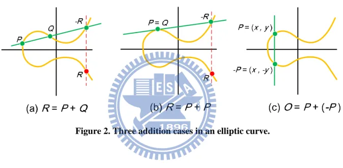
Let E is an elliptic curve over GF(p) which is defined as follows: where a, b GF(p) and

Let O mean the infinity. P(x1, y1) and Q(x2, y2) are two points on the curve and we compute R

= P + Q = (x3, y3) by following equations:

If P Q, it involves addition operations:

Table 1. Comparison of key lengths in different security levels [7]. RSA over binary field (bits) ECC over binary field (bits)

1024 160

2048 224

3072 256

7680 384

else if P = Q, it involves doubling operations

There are three addition cases in an elliptic curve that are shown in Figure 2. Those arithmetic operations over GF(p) consider about addition, subtraction, multiplication and inverse.

2.2 Elliptic curve Diffie-Hellman protocol

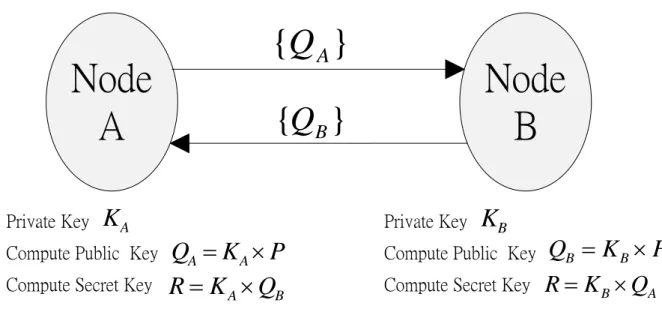
The traditional Elliptic Curve Diffie-Hellman Protocol (ECDH), which is based on the elliptic curve, works as shown in Figure 3.Initially, node A and node B both have the same elliptic curve E over GF(p) and the base point P which was suggested by NIST [15]. They generate their public keys, namely QA and QB, based on their private keys, KA and KB, by

multiplying P. After node A shares its public key to node B and node B shares its public key to node A, they generate secret key R where R = KA KB P. In ECDH, it is hard to be

figured out the private key (KA or KB) because deriving such a key is an elliptic curve discrete

logarithmic problem (ECDLP) [5] [6].

Node

A

Node

B

}

{

Q

_A

}

{

Q

P

K

Q





K

Q

K

R





Compute Public Key Compute Secret Key

B

K

P

K

Q





Q

K

R





Compute Public Key Compute Secret Key

Chapter 3

Related Work

ECC is a promising cryptography algorithm in WSNs; however, the scalar multiplications during key generation are the bottleneck. A few scalar multiplication schemes have been proposed to reduce the computation time. Some famous scalar multiplication schemes are briefly reviewed in the following sections.

3.1 Binary method [3]

The definition of scalar multiplication is the computation of the form Q = K P, where P and Q are two points on the elliptic curve and K is an integer [3]. K is converting into binary

K = , where kj {1, 0} is used to compute KP by repeatedly executing addition

and doubling operations and L is the bit lengths of binary K. The binary method scans the bits of K either from left-to-right or right-to-left. If kj = 1, then it needs to execute two operations,

one is doubling operation and the other is addition operation. If kj = 0, then it needs to execute

one doubling operation. In this method, the number of doubling operations is L – 1 and the number of addition operations is hw – 1 where hw is the Hamming weight defined as the number of none zero elements. The average Hamming weight is (L – 1) / 2. Thus, if a binary representation has more zeroes, the Hamming weight becomes smaller and the computation time becomes shorter. For example, if K = (1100111000111)2, then hw = 8. It will require

hw – 1 = 7 addition operations and L – 1 = 12 doubling operations.

3.2 Non-adjacent form [9]

requires the same operations with the Binary method. If kj = -1, then it needs to execute two

operations: doubling and subtraction, where subtraction is based on the addition operation but the associated point is changed from (x, y) to (x, -y). Here, we collectively called the subtraction as addition. The non-adjacent form (NAF) [9] is a signed binary representation and has no two consecutive non-zero digits in the representation. For example, if K = (1111)2,

then it is converted into K = . In NAF, the number of doubling operations is L – 1 and the number of addition operations is hw – 1. The average Hamming weight is (L – 1) / 3. Thus, NAF reduces the Hamming weight more than the Binary method and the computation time also becomes even shorter. NAF scans the bits of K from right-to-left and requires O(n) memory to store the shifted single digit. Hence, the conversion time of NAF is longer.

3.3 Mutual opposite form [10]

In 2004, Okeya [10] proposed a new scalar multiplication scheme called mutual opposite form (MOF). MOF is also a signed binary representation. The binary representation of K is converted into a signed binary representation by computing mi = ki-1 – ki where “ – ”

represents a bit wise subtraction [11]. The most significant bit is 1 and the least significant bit is -1. The conversion time of MOF is shorter than that of NAF because MOF just requires subtraction. And, MOF scans the bits of K either from right-to-left or left-to-right, which is more flexible. For example, let us take K = 6599 = (1100111000111)2, then K = 6599 =

(11001110001110)2 – (1100111000111)2 = ( )2 , where means -1.

3.4 Complementary recoding [12]

Complementary recoding was proposed by Chang et al. [12] in 2003. Complementary recoding is also a signed binary representation and it converts a binary string into a signed binary string by using complementary operation. The complementary operation is as follows:

, where kj {1, 0, -1} and is the inverse of K. For example,

if K = 1001, then .

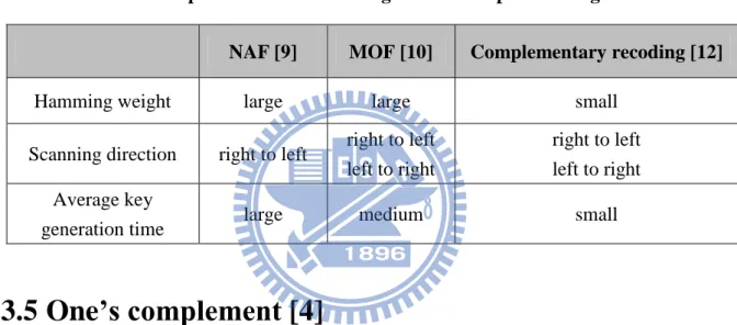
The conversion time of complementary recoding is shorter than that of MOF because the average Hamming weight of complementary recoding is smaller than that of MOF. That is, complementary recoding is faster than MOF. The qualitative comparison of the above three scalar multiplication algorithms is shown in Table 2. Note that the average key generation time is the average execution time of each algorithm [11].

3.5 One’s complement [4]

The window method [16] is different from the above three methods. It scans a few bits at a time and divides a binary string into several blocks. The sum of each block is odd and is less than 2w where w is the window size. Applying the window method to the elliptic curve cryptography will reduce the computation time and increase the memory usage and pre-computation time. Table 3 shows an example of K = 6599 = (1100111000111)2 with

different window sizes from 2 to 13. Note that when the window size increases, the number of pre-computed points will also increase geometrically. In addition, the number of addition and doubling operations will decrease and the computation time will decrease. Consequently, the selection of a window size will affect the computation time. It requires taking a tradeoff

Table 2. Comparison of three existing scalar multiplication algorithms.

NAF [9] MOF [10] Complementary recoding [12]

Hamming weight large large small Scanning direction right to left right to left

left to right

right to left left to right Average key

combines complementary recoding with the window method will largely reduces the average key generation time. However, it will consume more pre-computation time and memory due to the number of pre-computed points.

Table 3. Comparison of the numbers of pre-computed points and doubling and addition operations under different window sizes.

Window size Number of pre-computed points Number of doubling operations Number of addition operations 2 1 11 4 3 3 11 2 4 7 11 2 5 15 8 2 6 31 7 2 7 63 6 1 8 127 6 1 9 255 6 1 10 511 6 1 11 1023 2 1 12 2047 1 1 13 4095 0 0

Chapter 4

Proposed EW-MOF Algorithm

Because of limited resources in sensor nodes, we cannot use protocols with complicate computation in sensor nodes. Traditional ECC-based protocols, such as ECDH and ECDSA, take much computation time in scalar multiplication. In this paper, we propose an enhanced

window-based mutual opposite form for scalar multiplication (EW-MOF) for WSNs that can

largely reduce the number of pre-computed points and greatly reduce the computation time and memory usage in each sensor node. In Section 4.1, we describe why use MOF for scalar multiplication. The design of the proposed enhanced window method is described in Section 4.2. The proposed EW-MOF algorithm using the enhanced window method is described in Section 4.3.

4.1 Why use MOF for scalar multiplication

Because of using the window method, which scans several bits at a time, we need to compute 2w – 1 – 1 pre-computed points where w is the window size. For example, if w = 5, it requires to compute 25 – 1 – 1 = 15 pre-computed points, which are 3P, 5P, 7P, 9P, 11P, 13P, 15P, 17P, 19P, 21P, 23P, 25P, 27P, 29P and 31P. We have observed that existing scalar multiplication algorithms, such as NAF, MOF and one’s complement with window method, all may need to compute many pre-computed points. A large number of pre-computed points will increase pre-computation time and memory usage. In the following, we illustrate the above three scalar multiplication algorithms combined with the window method.

4.1.1 NAF

According to the NAF algorithm, there are no two consecutive non-zero digits in any representation. Thus, if w is odd, the maximal pre-computed point using NAF is

and if w is even, it wouldbe . For example, if w = 5, the maximal pre-computed point using NAF is and the pre-computed points are 3P, 5P, 7P, 9P, 11P, 13P, 15P, 17P, 19P, and 21P. Furthermore, if w = 6, the maximal pre-computed point using NAF is and the pre-computed points are 3P, 5P, 7P, 9P, 11P, 13P, 15P, 17P, 19P, 21P, 23P, 25P, 27P, 29P, 31P, 33P, 35P, 37P, 39P, and 41P.

4.1.2 MOF

Figure 4 shows the procedure of deriving pre-computed points for w = 5 in MOF. Note that the maximum pre-computed point is 15P and the number of pre-computed points is 7, which are 3P, 5P, 7P, 9P, 11P, 13P and 15P.

4.1.3 Complementary recording

Since complementary recording adopted one’s complement, the maximal pre-computed point would be , where means -1. For example, if w = 5, the maximal pre-computed point using complementary recording is and the pre-computed points are 3P, 5P, 7P, 9P, 11P, 13P, 15P,17P, 19P, 21P, 23P, 25P, 27P, 29P and 31P. 0 1 0 0 0 0 0 1 0 0 0 0 1-1 0 0 0 P 0 1 0 0 0 1 0 1 0 0 0 1 1-1 0 0 1 9P 0 1 0 0 1 0 0 1 0 0 1 0 1-1 0 1-1 9P 0 1 0 0 1 1 0 1 0 0 1 1 1-1 0 1 0 5P 0 1 0 1 0 0 0 1 0 1 0 0 1-1 1-1 0 5P 0 1 0 1 0 1 0 1 0 1 0 1 1-1 1-1 1 11P 0 1 0 1 1 0 0 1 0 1 1 0 1-1 1 0-1 11P 0 1 0 1 1 1 0 1 0 1 1 1 1-1 1 0 0 3P 0 1 1 0 0 0 0 1 1 0 0 0 1 0-1 0 0 3P 0 1 1 0 0 1 0 1 1 0 0 1 1 0-1 0 1 13P 0 1 1 0 1 0 0 1 1 0 1 0 1 0-1 1-1 13P 0 1 1 0 1 1 0 1 1 0 1 1 1 0-1 1 0 7P 0 1 1 1 0 0 0 1 1 1 0 0 1 0 0-1 0 7P 0 1 1 1 0 1 0 1 1 1 0 1 1 0 0-1 1 15P 0 1 1 1 1 0 0 1 1 1 1 0 1 0 0 0-1 15P 0 1 1 1 1 1 0 1 1 1 1 1 1 0 0 0 0 P 1 0 0 0 0 0 1 0 0 0 0 0 -1 0 0 0 0 -P 1 0 0 0 0 1 1 0 0 0 0 1 -1 0 0 0 1 -15P 1 0 0 0 1 0 1 0 0 0 1 0 -1 0 0 1-1 -15P 1 0 0 0 1 1 1 0 0 0 1 1 -1 0 0 1 0 -7P 1 0 0 1 0 0 1 0 0 1 0 0 -1 0 1-1 0 -7P 1 0 0 1 0 1 1 0 0 1 0 1 -1 0 1-1 1 -13P 1 0 0 1 1 0 1 0 0 1 1 0 -1 0 1 0-1 -13P 1 0 0 1 1 1 1 0 0 1 1 1 -1 0 1 0 0 -3P 1 0 1 0 0 0 1 0 1 0 0 0 -1 1-1 0 0 -3P 1 0 1 0 0 1 1 0 1 0 0 1 -1 1-1 0 1 -11P 1 0 1 0 1 0 1 0 1 0 1 0 -1 1-1 1-1 -11P 1 0 1 0 1 1 1 0 1 0 1 1 -1 1-1 1 0 -5P 1 0 1 1 0 0 1 0 1 1 0 0 -1 1 0-1 0 -5P 1 0 1 1 0 1 1 0 1 1 0 1 -1 1 0-1 1 -9P 1 0 1 1 1 0 1 0 1 1 1 0 -1 1 0 0-1 -9P 1 0 1 1 1 1 1 0 1 1 1 1 -1 1 0 0 0 -P

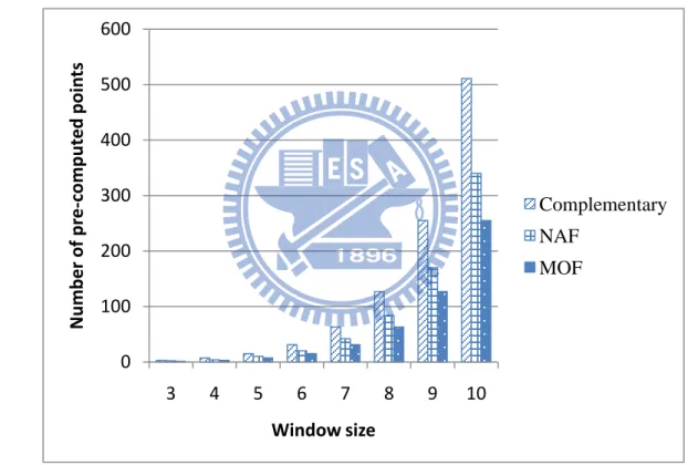
From the above, we found that MOF with window method has the smallest number of pre-computed points. Similarly, it has low pre-computation time and low memory usage. The comparison of number of pre-computed points under different window sizes among NAF, MOF, complementary recoding is shown in Figure 5. Note that the number of pre-computed points grows fast, especially for the complementary recording. MOF with window method has the smallest number of pre-computed points; therefore we choose MOF for scalar multiplication in order to reduce the number of pre-computed points and pre-computation time.

Figure 5. Comparison of the number of pre-computed points under different window sizes among NAF, MOF, complementary recoding.

0 100 200 300 400 500 600 3 4 5 6 7 8 9 10 Nu m b e r of p re -co m p u te d p oi n ts Window size Complementary NAF MOF

4.2 Design of the proposed enhanced window method

In this section, we propose an enhanced window method that can significantly reduce the number of pre-computed points than the original window method. The enhanced window method only requires to compute a few essential pre-computed points which can then be used to derive the rest of pre-computed points at low cost. The enhanced window method for deriving essential pre-computed points is described in Figure 6.

We select S that can result in the smallest number of essential pre-computed points for a specific window size. Based on the essential pre-computed points, we can derive the rest of pre-computed points. That is, we can calculate remaining pre-computed points by adding or subtracting two selected essential pre-computed points. Only one extra addition time is needed to calculate a pre-computed point. Furthermore, once a pre-computed point has been derived, it will be saved in a sensor node. If we need this pre-computed point later, we do not need to calculate it again. Hence, no extra addition time is consumed. The enhanced window method can largely reduce the total number of essential pre-computed points (Ne) and

Essential pre-computed points =

The constraints are:

1) S is the number of even essential pre-computed points and S 1.

2) {The maximal essential pre-computed point + _{(the maximal}

pre-computed point). 3) w 4.

In the following, we give an example to illustrate the selection of S for w = 6 using MOF. Note that the maximal pre-computed point is 31P:

For S = 1

Essential pre-computed points = {2P} {5P, 11P, 17P, 23P, 29P} = {2P, 5P, 11P, 17P, 23P, 29P} such that (29P + 2P) 31P

The total number of essential pre-computed points = 6

For S = 2

Essential pre-computed points = {2P, 4P} {7P, 17P, 27P} = {2P, 4P, 7P, 17P, 27P} such that (27P + 4P) 31P

The total number of essential pre-computed points = 5

For S = 3

Essential pre-computed points = {2P, 4P, 6P} {9P, 23P, 37P} = {2P, 4P, 6P, 9P, 23P, 37P} such that (37P + 6P) 31P

The total number of essential pre-computed points = 6

Since the number of essential pre-computed points for S = 2 is the smallest, S = 2 is selected. Therefore, all pre-compute points, 3P, 5P, 7P, 9P, 11P, 13P, 15P, 17P, 19P, 21P, 23P, 25P, 27P, 29P, 31P, can be derived from essential pre-computed points = {2P, 4P, 7P, 17P, 27P}. The details are as follows: Firstly, 3P, 11P can be calculated by and 5P, 9P can be calculated by . Secondly, 13P, 21P can be calculated by and 15P, 19P can be calculated by . Thirdly, 23P, 31P can be calculated by 2 and 25P, 29P can be calculated by 2 . Therefore, we have obtained all pre-computed points. By using the proposed enhanced window method, the number of essential pre-computed points that need to be derived initially has been reduced from 15 to 5. However,

extra additions will be needed for calculating the rest of pre-computed points when needed, which is a small overhead. The best selection of S under different window sizes is shown in Table 4. Figure 7 shows the comparison of the number of essential pre-computed points under different window sizes in MOF using the window method and the enhanced window method. Note that the number of essential pre-computed points using the enhanced window method is much smaller than that of the window method. As the window size increases, the improvement will become significant.

Figure 7. Comparison of the number of essential pre-computed points under different

0 50 100 150 200 250 300 4 5 6 7 8 9 10 Nu m b e r of e ssen ti al p re -co m p u te d p oi n ts Window size Window method Enhanced window method (proposed)

Table 4. Best selection of S under different window sizes.

w 4 5 6 7 8 9 10

Figure 8 shows the selection of the best window size under N (assuming 100) times of key generations. Essential pre-computed points ratio is defined as the number of essential pre-computed points divided by the total number of pre-computed points. Average number of

extra additions in each key generation is defined as the number of extra addition operations

divided by N (= 100, in this case). We found that the best window size is w = 6 under 100 times of key generations. If N is larger than 100, the best window size will increase.

4.3 Design the proposed EW-MOF algorithm

In this section, we propose an enhanced window-based mutual opposite form for scalar multiplication (EW-MOF) in WSNs. The proposed EW-MOF combines MOF with an enhanced window method that can significantly not only reduce the number of essential pre-computed points but also reduce memory consumption and speed up the average key generation time. The proposed EW-MOF algorithm is shown in Algorithm 1, which includes

Figure 8. Selection of the best window size under N (assuming 100) times of key generations. 0 0.5 1 1.5 2 2.5 3 4 5 6 7 8 9 10 Windowsize Essential pre-computed points ratio Average number of extra additions

three phases, essential pre-computed points pre-computation phase, signed binary

representation phase and public key generation using enhanced window method phase. In the

essentialpre-computed points pre-computation phase, all the essential pre-computed points will be calculated once S is selected for a specific window size. After the essential pre-computed points pre-computation phase, we start to execute the scalar multiplication algorithm to calculate the public key. In the signed binary representation phase, the private key utilizes MOF to convert the binary representation into a signed binary representation. Then, the public key is calculated in the public key generation using enhanced window method phase. Firstly, the private key is scanned from left to right. If a digit is 0, doubling operations are executed; otherwise, remove the block based on the window size. If the sum of the block has been saved in the sensor node, addition operations are executed to calculate the public key. If the sum of the block has not been saved in the sensor node, addition operations are executed to calculate the sum of the block first by using essential pre-computed points and save it in the sensor node. Then, addition operations are executed to calculate the public key. In addition, if we have another block with the same sum later, no more calculation is needed. Finally, the execution will continue until the end of digits and the public key is returned.

Algorithm 1: Left-to-Right EW-MOF

Input: An n-bit binary string K = bn-1,bn-2, …, b1, b0, where K is a private key and w

Output: A public key Q, where Q = KP

1. Essential pre-computed points pre-computation phase:

1.1 S = Table lookup (w) 1.2 P1 = P, P2 = 2P, P3+2S = (3 + 2S)P, P2+4S= (2 + 4S)P 1.3 i = 4, j = 5 + 6S, r = Ne – S 1.4 While S > 1 do Pi = Pi-2 + P2, i = i + 2, and S = S – 1 1.5 While r > 1 do Pj = Pj-(2+4S)+ P2+4S, j = j + (2 + 4S), and r = r – 1 2. Signed binary representation phase:

2.1 mn = bn-1

2.2 For i = n – 1 down to 1 do

mi = bi-1– bi

2.3 m0 = –b0

3. Public key generation using enhanced window method phase:

3.1 Q = P 3.2 While do 3.2.1 If mn = 0 then Q = 2Q and n = n – 1 3.2.2 Else g = max(n – w + 1, 0) While mg = 0 do g = g + 1 wsum = 0 For i = n to g do Q = 2Q wsum = 2wsum + mi

If Pwsum has been calculated

Q = Q + Pwsum

Else

calculate Pwsum by essential pre-computed points

save Pwsum in the sensor node

Q = Q + Pwsum

3.2.3 n = g – 1 3.3 Return Q

Figure 9 shows the flowchart of selecting an elliptic curve and a base point (P(x, y)) for ECC in wireless sensor networks. Firstly, the sink selects an elliptic curve over GF(p) where a, b GF(p) and . Then, the sink selects a base point P = (x, y) on the elliptic curve, where x and y are the coordinates of E. When a sensor node receives the elliptic curve and the base point, it will determine a window size w and executes the essential pre-computed points pre-computation phase. After this phase, these essential pre-computed points will be stored in the sensor node. If the elliptic curve E or the base point P is changed, the essentialpre-computed points pre-computation phase needs to be re-executed and new essential pre-computed points are stored in the sensor node. In this paper, we assume all computations are performed in the sensor node, since it would be more secure to do key exchanges and key generations in WSNs.

Figure 10 shows the flowchart of the public key generation process for a sensor node. The sensor node generates a private key K and executes the signed binary representation phase to convert K into m in MOF. Then, according to window size w, m is split into several blocks. Then, the sensor node checks whether the sum of the block has been saved or not. If the sum of the block has been saved, the sensor node will compute public key Q using the proposed enhanced window method. Otherwise, the sensor node will execute addition operations to derive the sum of the block from essential pre-computed points and save it in the sensor node. Then, the sensor node computes public key Q using the enhanced window method. Finally, public key Q is calculated.

 

₄



₂₇



₀

b

a

 

p

GF

In the following, we give an example to illustrate how a sensor node computes a public key Q. For w = 6, essential pre-computed points = {2P, 4P, 7P 17P, 27P}. Firstly, the sensor node randomly generates a private key K = 12434877 = (101111011011110110111101)2.

Express K in MOF:

Note that 3P can be calculated by 7P – 4P, which only needs to be calculated once and 9P can be calculated by 7P + 2P, which again only needs to be calculated once. The intermediate values of Q are 3P, 6P, 12P, 24P, 48P, 96P, 192P, 384P, 768P, 759P, 1518P, 3036P, 6072P, 12144P, 24288P, 48576P, 97152P, 194304P, 194295P, 388590P, 777180P, 1554360P, 3108720P, 6217440P, 12434880P, 12434877P

The computation cost of arithmetic operations for the above example include 22 doubling operations, 5 addition operations, with two extra addition operations used to calculate 3P and 9P. Although two extra addition operations are needed, there is no need to calculate them again at next time. Note that the two extra addition operations will result in very small increase in the average key generation time since the average extra number of additions for w = 6 is very small, as shown previously. That is, the time required for the two extra addition operations in the average key generation time can be neglected.

Chapter 5

Performance Evaluation and Discussion

In this chapter, we evaluate the average key generation time of the proposed EW-MOF and compare it with that of one’s complement.

5.1 Simulation environment setup

We implemented the proposed EW-MOF on the 2.66 GHz Intel Core i5 and used Multiprecision Integer and Rational Arithmetic C/C++ Library (MIRACL) [13] for elliptic curves and Basicrypt which is an ECC benchmark suite [14] for ECC. MIRACL is a big number library which implements all of the primitives necessary to design big number cryptography into your real-world application [13]. It is an open source library and can be used to perform the arithmetic of elliptic curves. The Basicrypt benchmark package uses the MIRACL library and it contains standards and elliptic curve codes for Diffie-Hellman key exchange, digital signature algorithm, ElGamal and RSA encryption/decryption [14]. Furthermore, the various parameters of elliptic curves are defined in the National Institute of Standards and Technology (NIST) DSS standard FIPS 186-3 [15].

5.2 Comparison between the proposed EW-MOF and

one’s complement

Figure 11 shows the average key generation time, excluding pre-computation time, of the binary, MOF, one’s complement, and the proposed EW-MOF methods under different field sizes for w = 6. The average key generation time is defined as the summation of each key generation time divided by the number of key generations (N). The field size means the

elliptic curves over prime fields that are specified in [15]. The average key generation time of Binary is the worst because Binary contains the most bits of 1 that involve addition and doubling operations. The average key generation time of MOF is better than that of Binary because MOF contains less bits of 1. As to the one’s complement, the average key generation time is better than that of MOF because one’s complement uses the window method that splits the private key into blocks so as to reduce the number of addition operations. The proposed EW-MOF is almost the same as one’s complement because their numbers of blocks are not much different. As a result, their numbers of addition operations are not much different. Although the proposed EW-MOF requires extra addition operations, it causes little increase in the average key generation time.

Figure 12 shows the average key generation time, including pre-computation time, of the one’s complement and the proposed EW-MOF under different field sizes for w = 6. The average key generation time of the proposed EW-MOF is better than that of the one’s

Figure 11. Average key generation time excluding pre-computation time under different field sizes. 2 3 4 5 6 7 8 9 10 192 224 256 384 521 A ve ra ge k ey g e n e ra ti on ti m e (m s)

Field size (bit)

Binary MOF One's complement (window size 6) EW-MOF (proposed) (window size 6)

complement because the number of pre-computed points in the one’s complement is larger than that of the proposed EW-MOF, as shown in Figure 5 and Figure 7. Thus, the pre-computation time in the one’s complement is longer than that of the proposed EW-MOF. In summary, in terms of the average key generation time, including pre-computation time, under different field sizes, for w = 6, the proposed EW-MOF is 24.69% faster than the one’s complement.

Figure 13 shows the average key generation time, excluding pre-computation time, of the one’s complement and the proposed EW-MOF under different window sizes. We found that when the window size increases the average key generation time decreases. This is because when the window size increases the number of blocks will decrease and the number of addition operations will decrease as well. The average key generation time of the one’s complement and the proposed EW-MOF are almost the same for . This matches the

Figure 12. Average key generation time including pre-computation time under different field sizes. 2 2.5 3 3.5 4 4.5 5 5.5 6 6.5 7 192 224 256 384 521 A ve ra ge k ey g e n e ra ti on ti m e (m s)

Field size (bit)

One's complement (window size 6)

EW-MOF

(proposed) (window size 6)

generations. For , the average key generation time of the proposed EW-MOF will slowly increase. This is because that the proposed EW-MOF has a smaller number of essential pre-computed points. However, for the same number of pre-computed points, the proposed EW-MOF can set a bigger window size than one’s complement. Thus, the proposed EW-MOF can be still faster than the one’s complement in terms of average key generation time, excluding pre-computation time.

Figure 14 shows the average key generation time, including pre-computation time, of the one’s complement and the proposed EW-MOF under different window sizes. The average key generation time of the proposed EW-MOF is better than that of the one’s complement because the number of pre-computed points in the one’s complement is larger than that of the proposed EW-MOF, as shown in Figure 7. Note that the average key generation time of the proposed EW-MOF increases slowly compared to that of the one’s complement as window

Figure 13. Average key generation time, excluding pre-computation time, under different window sizes.

2.2 2.3 2.4 2.5 2.6 2.7 2.8 4 5 6 7 8 9 10 A ve ra ge e k ey g e n e ra ti on ti m e (m s) Window size One's complement EW-MOF (proposed)

size increases. This is because the number of essential pre-computed points does not increase too much in the proposed EW-MOF; however, the number of pre-computed point increases exponentially in the one’s complement.

5.3 Discussion

Since the proposed EW-MOF is 24.69% faster than the one’s complement in terms of average key generation time, the proposed EW-MOF is more power saving than the one’s complement. That is, the proposed EW-MOF is more feasible than the one’s complement for wireless sensor networks, which is battery powered, in terms of power saving. Applying the proposed EW-MOF to the ECC for wireless sensor networks can benefit associated sensor nodes in terms of less computing and memory needed, and power saving. In addition, the proposed EW-MOF is also feasible to other mobile and wireless devices for ECC security.

Figure 14. Average key generation time, including pre-computation time, under different window sizes.

0 5 10 15 20 25 30 4 5 6 7 8 9 10 A ve ra ge k ey g e n e ra ti on ti m e (m s) Window size One's complement EW-MOF (proposed)

Chapter 6

Conclusion

6.1 Concluding remarks

In this paper, we have presented an enhanced window-based mutual opposite form for scalar multiplication (EW-MOF) that combines MOF with an enhanced window method. The proposed EW-MOF can largely reduce average key generation time including pre-computation time and it needs less pre-computation time and memory. Moreover, the proposed enhanced window method only requires to calculate essential pre-computed points, which is better than the original window method that needs to calculate all pre-computed points. Simulation results have shown that the proposed EW-MOF is 24.69% faster than the one’s complement in terms of average key generation time including pre-computation time under different field sizes. Furthermore, the proposed EW-MOF can use a larger window size because its number of essential pre-computed points is smaller than the number of pre-computed points used in the one’s complement. Thus, the average key generation time, excluding pre-computation time, of the proposed EW-MOF can be still shorter than that of the one’s complement. Shorter average key generation time implies consuming less power, which is important for wireless sensor networks that are battery-powered. The proposed EW-MOF can significantly reduce ECC key generation time and is suitable for wireless sensor networks. That is, the proposed EW-MOF is more feasible than the one’s complement for wireless sensor networks in terms of key generation time and power saving.

6.2 Future work

The proposed EW-MOF can be applied to key exchange protocols, such as ECDH and ECDSA, for security and power saving of wireless sensor networks. In addition, we can apply the proposed EW-MOF to any wireless network that uses elliptic curve cryptography for reducing key generation time and power consumption.

Bibliography

[1] E. K. Wang and Yunming Ye, "An Efficient and Secure Key Establishment Scheme for Wireless Sensor Network," in Proc. Intelligent Information Technology and Security

Informatics, pp. 511-516, Apr. 2010.

[2] W. Stallings, Cryptography and Network Security- Principles and Practices, 3rd Ed. NJ: Prentice Hall, 2003.

[3] E. Karthikeyan and P. Balasubramaniam, "Improved Elliptic Curve Scalar Multiplication Algorithm," in Proc. IEEE International Conference on Information and Automation, pp. 254-257, Dec. 2006.

[4] P. G. Shah, Xu Huang, D. Sharma, "Algorithm Based on One's Complement for Fast Scalar Multiplication in ECC for Wireless Sensor Network," in Proc. IEEE 24th

International Conference on Advanced Information Networking and Applications Workshops, pp. 571-576, Apr. 2010.

[5] V.S. Miller, "Use of Elliptic Curves in Cryptography," in Proceedings of Advances in

Cryptology – CRYPTO '85, vol. 218: Springer-Verlag, pp. 417-426, 1986.

[6] N. Koblitz, "Elliptic Curve Cryptosystems," in Proceedings of Mathematics of

Computation, vol. 48, pp. 203-209, 1987.

[7] NIST, DRAFT Special Publication 800-57, Recommendation for Key Management, Mar

2007, Available at

http://csrc.nist.gov/publications/nistpubs/800-57/sp800-57-Part1-revised2_Mar08-2007.pd f.

[8] A.D. Booth, "A Signed Binary Multiplication Technique," in Journal of Applied

Mathematics, vol. 4, pp. 236-240, 1951.

Addition–Subtraction Chains," in Proceedings of RAIRO Theoretical Informatics and

Applications, vol. 24, pp. 531-543, 1990.

[10] K. Okeya, "Signed Binary Representations Revisited," in Proceedings of CRYPTO’04, pp. 123-139, 2004.

[11] P. Balasubramaniam and E. Karthikeyan, "Elliptic Curve Scalar Multiplication Algorithm Using Complementary Recoding," in Proceedings of Mathematics and

Computation, Jan.2007.

[12] C.C. Chang, Y.T. Kuo, and C.H. Lin, "Fast Algorithms for Common Multiplicand Multiplication and Exponentiation by Performing Complements," in Proceeding of 17th

International Conference on Advanced Information Networking and Applications, pp.

807-811, Mar. 2003.

[13] MIRACL, Multiprecision Integer and Rational Arithmetic C/C++ Library, Available at

http://www.shamus.ie/.

[14] Basicrypt, Elliptic Curve Cryptography Benchmark Suite, Available at

http://www.dii.unisi.it/~giorgi/basicrypt/.

[15] NIST, Digital Signature Standard FIPS PUB 186-3, Available at

http://csrc.nist.gov/publications/fips/fips186-3/fips_186-3.pdf, 2009.

[16] J. Lopez and R. Dahab, "An overview of elliptic curve cryptography," Technical Report, Institute of Computing, State University of Campinas, Brazil, May 2000.