591
⁄
0743-7315/02 $35.00© 2002 Elsevier Science (USA) All rights reserved.
Fault-Tolerant Hamiltonicity of Twisted Cubes
11This work was supported in part by the National Science Council of the Republic of China under
Contract NSC 89-2213-E-009-13. Correspondence should be addressed to Professor Jimmy J. M. Tan, Department of Computer and Information Science, National Chiao Tung University, Hsinchu, Taiwan 300, R.O.C. E-mail: [email protected].
Wen-Tzeng Huang, Jimmy J. M. Tan, Chun-Nan Hung, and Lih-Hsing Hsu
Department of Computer and Information Science, National Chiao Tung University, Hsinchu, Taiwan 300, Republic of China
E-mail: [email protected]
Received September 23, 1999; revised May 15, 2000; accepted October 23, 2001
The twisted cube TQn, is derived by changing some connection of
hyper-cube Qn according to specific rules. Recently, many topological properties of
this variation cube are studied. In this paper, we consider a faulty twisted
n-cube with both edge and/or node faults. Let F be a subset of V(TQn) 5
E(TQn), we prove that TQn− F remains hamiltonian if |F| [ n − 2. Moreover,
we prove that there exists a hamiltonian path in TQn− F joining any two
vertices u, v in V(TQn) − F if |F| [ n − 3. The result is optimum in the sense
that the fault-tolerant hamiltonicity (fault-tolerant hamiltonian connectivity respectively) of TQnis at most n − 2 (n − 3 respectively). © 2002 Elsevier Science (USA)
Key Words: hamiltonian; hamiltonian connected; fault-tolerant; twisted
cube.
0. INTRODUCTION AND NOTATION
The architecture of an interconnection network is usually represented by a graph. We use graphs and networks interchangeably. There are a lot of mutually conflict-ing requirements in designconflict-ing the topology of interconnection networks. It is almost impossible to design a network which is optimum from all aspects. One has to design a suitable network depending on the requirements and its properties. The hamiltonian property is one of the major requirements in designing the topology of networks. Fault tolerance is also desirable in massive parallel systems that have relatively high probability of failure.
A network is represented as an undirected graph in this paper. For the graph theoretic definition and notation we follow [5]. G=(V, E) is a graph if V is a finite set and E is a subset of {(a, b) | (a, b) is an unordered pair of V}. We say that V is the vertex (or node) set and E is the edge (or link) set. Two nodes a and b are
adjacent. A path is represented byOv0Qv1Qv2... Q vk − 1P. We also write the path
Ov0Qv1Qv2... Q vk − 1P as Ov0QP1QviQvi+1... Q vjQP2QvtQvt+1... Q vk − 1P,
where P1=Ov0Qv1... Q viP and P2=OvjQvj+1... Q vtP. A path is a hamiltonian
path if its nodes are distinct and they span V. A cycle is a path with at least three
nodes such that the first node is the same as the last node. A cycle is called a
hamil-tonian cycle if it traverses every node of G exactly once. A graph is hamilhamil-tonian if
it has a hamiltonian cycle. Let G0=(V0, E0) and G1=(V1, E1) be two graphs.
Following the definition [17], the Cartesian product of G0 and G1, denoted by
G0× G1, is the graph with the vertex set V0× V1 such that (x, y) ¥ E(G0× G1) with
x=(vx 0, v x 1) and y=(v y 0, v y
1) if and only if either (v x 0=v y 0 and (v x 1, v y 1) ¥ E(G1)) or (vy 1=vy1and (vx0, vy0) ¥ E(G0)).
Since node faults and link faults may happen when a network is used, it is prac-tically meaningful to consider faulty networks. The vertex fault-tolerant hamiltoni-city and the edge fault-tolerant hamiltonihamiltoni-city, proposed by Hsieh et al. [10], measure the performance of the hamiltonian property in the faulty networks. The
vertex fault-tolerant hamiltonicity, Hv(G), is defined to be the maximum integer k
such that G − F remains hamiltonian for every F … V(G) with |F| [ k if G is hamil-tonian and undefined if otherwise. Obviously, Hv(G) [ d(G) − 2 where d(G)=
min{deg(v) | v ¥ V(G)}. Similarly, the edge fault-tolerant hamiltonicity, He(G), is
defined to be the maximum integer k such that G − F remains hamiltonian for every
F … E(G) with |F| [ k if G is hamiltonian and undefined if otherwise. Again, it is
obvious that He(G) [ d(G) − 2. Many topological properties of graphs have been
studied [9, 10, 12, 13, 15, 16]. In [10], Hsieh et al, showed that an arrangement graph An, k remains hamiltonian if the parameters n and k satisfy some conditions
and the total number of edge and/or vertex faults is not more than a certain amount, for example, k(n − k) − 2, n − 3, or k. In [12], Latif et al. demonstrated that an n-dimensional hypercube with at most n − 2 link faults is hamiltonian. In [13], Rowley and Bose showed that, with slight modification, a base-d undirected de Bruijn graph with at most d − 1 edges faults is hamiltonian. In [15], Sung et al. demonstrated that a double loop network, which is a digraph with n nodes and 2n links, with a node or a link fault is hamiltonian. In [16], Tseng et al. proved that an
n-dimensional star graph with at most n − 3 edge faults is hamiltonian. In [9],
Huang et al. proposed a preliminary result of our current study in this paper. In this paper, we consider a more general parameter. The fault-tolerant
hamilto-nicity, Hf(G), is defined to be the maximum integer k such that G − F remains
hamiltonian for every F … V(G) 2 E(G) with |F| [ k if G is hamiltonian and undefined if otherwise. Obviously, Hf(G) [ min{Hv(G), He(G)} [ d(G) − 2. For
technical reasons, we also introduce the term fault-tolerant hamiltonian connectivity. A graph G is hamiltonian connected if there exists a hamiltonian path joining any two vertices of G. The fault-tolerant hamiltonian connectivity, Ho
f(G), is defined to
be the maximum integer k such that G − F remains hamiltonian connected for every
F … V(G) 5 E(G) with |F| [ k if G is hamiltonian connected and undefined if
otherwise. Obviously, Ho
f(G) [ d(G) − 3. A graph G is called k-fault-tolerant
hamiltonian (k-fault-tolerant hamiltonian connected, respectively) or simply k-hamil-tonian (k-hamilk-hamil-tonian connected, respectively) if it remains hamilk-hamil-tonian (hamilk-hamil-tonian
Among all interconnection networks proposed in the literature, the hypercube Qn
is one of the most popular topologies. Twisted cube [8], TQn, is derived by
chang-ing some connections of hypercube Qn according to specific rules. Recently, many
topological properties of this variation cube have been studied: In [8], Hilbers et al. first defined the twisted cubes. In [1], Abraham and Padmanabhan proved that the twisted cube supported a better performance than that of the hypercube, although it is an asymmetry network. In [2], Abuelrub and Bettayeb demonstrated that a complete binary tree can be embedded in the twisted cube. In [6], Chang et al. showed that the connectivity of the twisted cube TQn, is n, the wide diameter and
the fault diameter areKn
2L+2, and the twisted cube is a pancyclic network. All these
results indicate that the performance of TQnis better than that of Qn in the
condi-tions mentioned in those papers.
In this paper, we prove that TQn still remains hamiltonian (hamiltonian
con-nected, respectively), even if it has up to n − 2 (n − 3, respectively) edge and/or node faults. This result is optimum in the sense that the tolerant hamiltonicity ( fault-tolerant hamiltonian connectivity, respectively) of TQn is at most n − 2 (n − 3,
respectively). Therefore, Hf(TQn)=n − 2 and H o
f(TQn)=n − 3, for n \ 3 and n is
odd. In contrast with the hypercube, the grid, the mesh, and the torus, the fault-tolerant hamiltonicity property of the twisted cubes is much better. For hypercube network Qn, it is proved in [12, 14] that the vertex fault-tolerant hamiltonicity of
Qn is equal to 0 and the edge fault-tolerant hamiltonicity of Qn is equal to n − 2.
Thus, the fault-tolerant hamiltonicity of Qnis equal to 0 if n \ 2. For the grid [3],
the mesh [11], and the torus [4, 7] with 2n vertices, because they are bipartite
graphs, there are no hamiltonian cycles even if there is only one vertex fault in these graphs. Therefore, the vertex fault-tolerant hamiltonicity of these graphs is equal to
0. So the fault-tolerant hamiltonicity of these graphs with 2nvertices is equal to 0.
1. TWISTED CUBE AND ITS PROPERTIES
The vertex set of the twisted n-cube TQn, is the set of all binary strings of length
n. Let u=un − 1un − 2...u1u0 be any vertex in TQn. For 0 [ i [ n − 1, we define the ith
parity function Pi(u)=uiÀui − 1À · · · À u0, where À is the exclusive-or operation.
When twisted cube was first defined by Hibers et al. [8], the authors only con-sidered twisted n-cubes TQn for odd values of n exclusively. Following the
defini-tion in [8], we can recursively define TQn as follows: A twisted 1-cube, TQ1, is a complete graph with two vertices 0 and 1. Suppose that n \ 3. We can decompose the vertices of TQn into four sets, TQ0, 0n − 2, TQ
0, 1 n − 2, TQ 1, 0 n − 2 and TQ 1, 1 n − 2 where TQ i, j n − 2
consists of those vertices u with un − 1=i and un − 2=j. For each (i, j) ¥
{(0, 0), (0, 1), (1, 0), (1, 1)}, the induced subgraph of TQi, j
n − 2 in TQn is isomorphic
to TQn − 2. Edges which connect these four subtwisted cubes can be described as
follows: Any node U=un − 1un − 2· · · u1u0 with Pn − 3(U)=0 is connected to V=
vn − 1vn − 2· · · v1v0, where V=u¯n − 1u¯n − 2un − 3· · · u1u0 or V=u¯n − 1un − 2un − 3· · · u1u0; a node
U with Pn − 3(U)=1 is connected to V, where V=un − 1u¯n − 2un − 3· · · u1u0 or V=
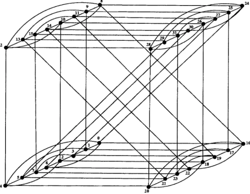
u¯n − 1un − 2un − 3· · · u1u0. TQ3and TQ5are shown in Figs. 1 and 2, respectively.
FIG. 1. Twisted 3-cube TQ3.
Lemma 1.1. Both the subgraph induced by TQ0, 0n − 22TQ1, 0n − 2 and the subgraph
induced by TQ0, 1 n − 22TQ
1, 1
n − 2 are isomorphic to TQn − 2× K2 where K2 is the complete
graph with two vertices. Moreover, the edges joining TQ0, 0
n − 22TQ1, 0n − 2 and TQ0, 1n − 22
TQ1, 1
n − 2 form a perfect matching of TQn.
2. HAMILTONIAN CYCLES IN FAULTY TWISTED CUBE
Let G0and G1be two graphs with the same number of nodes, and let M be an
arbitrary perfect matching between the nodes of G0and G1; i.e., M is a set of edges
connecting the nodes of G0and G1in a one to one fashion.In this paper, we define a
connection graph G0À
MG1as follows, where G0=G1=G. It has two copies of G
connected by a matching M; these two copies of G, denoted by G0 and G1, are
called two sides of G0À
M G1 which has vertex set V(G0ÀMG1)=V(G0) 2 V(G1)
and edge set E(G0À
MG1)=E(G0) 2 E(G1) 2 M. The matching edges connecting
G0 and G1 are called crossing edges. For each node u of G, u0and u1 are used to
denote its two copies in G0and G1, and are called corresponding nodes of G0and G1.
We also say that the corresponding node of u0is u1. Observe that the product graph
G × K2 is also a connection graph G ÀM G. Using the above terminologies, G × K2
has two sides G0 and G1 connected by matching M={(u0, u1) | u ¥ V(G)}. Also
TQn=(TQn − 2× K2) ÀM(TQn − 2× K2) for a specific perfect matching M.
We will prove that the twisted n-cube TQn, for n \ 3, has a hamiltonian cycle even if it has up to n − 2 vertex and/or edge faults. In fact, we will prove a stronger result: TQnis (n − 2)-hamiltonian and (n − 3)-hamiltonian connected for n \ 3. The
basic idea of our proof is by induction on n, and the outline of our proof is as follows: First, we observe that TQ3 is 1-hamiltonian and hamiltonian connected.
Then, assuming the result is true for TQk, for 3 [ k [ n, we show that TQn× K2 is
(n − 1)-hamiltonian and (n − 2)-hamiltonian connected. Finally, we prove that
TQn+2=(TQn× K2) ÀM(TQn× K2) is n-hamiltonian and (n − 1)-hamiltonian
con-nected, and this completes the induction proof. To start our induction, let us look at the twisted 3-cube TQ3.
In Figs. 3a and 3b, there are two different but equivalent layouts of TQ3, where
the binary node labels are represented by their corresponding decimal numbers. By the node symmetry of TQ3, it is a simple matter to check that TQ3is indeed
hamil-tonian connected. For example, ‘‘0-1-3-2-4-5-7-6,’’ ‘‘0-6-2-4-5-1-3-7,’’ ‘‘0-1-3-7-6-2-4-5,’’ and ‘‘0-1-3-2-6-7-5-4’’ are hamiltonian paths between nodes and 6, 0 and 7, 0 and 5, and 0 and 4, respectively.
Again by the symmetry of Fig. 3b, we can check that TQ3is 1-hamiltonian. For
example, if node 1 is faulty, then ‘‘0-6-2-3-7-5-4-0’’ is a fault-free hamiltonian cycle. Moreover, ‘‘0-4-2-3-1-5-7-6-0’’ is a hamiltonian cycle not using edges (0, 1), (2, 6),
(3, 7) and (4, 5). Therefore, we have the following lemma.
Lemma 2.2. Twisted 3-cube TQ3is hamiltonian connected and 1-hamiltonian. As another example, TQ5 shown in Fig. 2 is labeled by a decimal number. We
can show that TQ5 is 2-hamiltonian connected and 3-hamiltonian by applying
Theorem 2.2. However, to get some intuition about the results, we check some cases
that TQ5 is 2-hamiltonian connected. For example, if nodes 0 and 16 are faulty,
‘‘1-3-2-6-7-5-4-12-8-9-11-10-14-15-13-21-17-19-23-22-18-20-28-29-25-24-30-26-26-27-31’’ and ‘‘1-5-4-2-3-7-6-30-26-27-31-29-28-24-25-17-21-20-18-19-23-22-14-8-9-11-10-12-13-15’’ are fault-free hamiltonian paths between nodes 1 and 31 and nodes 1 and 15, respectively. Moreover, we can also check that TQ5 is 3-hamiltonian. For
example, if nodes 0, 8, and 16 are faulty, then ‘‘1-3-2-6-7-5-4-20-21-23-22-18-19-17-25-24-30-26-27-31-28-12-1 3-15-14-10-11-9-1’’ or ‘‘1-3-2-6-7-5-4-12-13-15-14-10-11-9-25-24-30-26-27-31-29-28-20-21-23-22-18-19-17-1’’ is a fault-free hamiltonian cycle in TQ5.
To prove Theorem 2.1, we shall make use of the structure of TQn× K2. Let TQ 0 n
and TQ1
n be the two sides of TQn× K2; each side TQin (isomorphic to TQn) has 2n
nodes, i=0, 1. And TQ0
nand TQ 1
nare connected by matching corresponding nodes.
Recall that, for each node u of TQn, u0 and u1 are used to denote
correspond-ing nodes of TQ0
n and TQ 1
n. These notations are used extensively throughout
Theorem 2.1.
Theorem 2.1. Let n be a fixed odd integer and n \ 3. If TQn is (n −
2)-hamiltonian and (n − 3)-2)-hamiltonian connected, then TQn× K2 is (n − 1)-hamiltonian
and (n − 2)-hamiltonian connected.
Proof. Let Ec be the set of crossing edges; that is, Ec={(u0, u1) | -u ¥ TQn}. Let
F be a faulty set, F0=F 5 TQ
0
n, F1=F 5 TQ
1
n, and Fc=F 5 Ec. And the
cardi-nalities of F0, F1, Fc are f0, f1, fc, respectively. In the following, we shall use the
notation HPi(ui, vi) (Pi(ui, vi)respectively) to denote a hamiltonian path (a path,
respectively) in the graph TQi
n− Fi joining uiand vifor i=0, 1, and HCito denote
a hamiltonian cycle in TQi
n− Fi for i=0, 1.
First, we prove that TQn× K2 is (n − 1)-hamiltonian. We will prove that
(TQn× K2) − F has a hamiltonian cycle if F … (V(TQn× K2) 2 E(TQn× K2)) and
|F|=n − 1 with the following two cases.
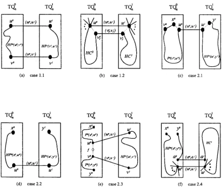
Case 1.1. fi=n − 1 for some i=0, 1. (All faults are on one side. See Fig. 4a).
Without loss of generality, we assume that f0=n − 1. Since TQ0n is (n −
2)-hamiltonian, there exists a hamiltonian path HP0(u0, v0) joining some two vertices
u0, v0in TQ0
n− F. Since TQ1n is hamiltonian connected, there exists another
hamil-tonian path HP1(u1, v1) in TQ1
n, where uiand v1are the corresponding nodes of u0
and v0, respectively. Then, Ou0QHP0(u0, v0) Q v0Qv1QHP1(v1, u1) Q u1Qu0P
forms a hamiltonian cycle in (TQn× K2) − F.
Case 1.2. fi[n − 2 for i=0, 1. (All faults are scattered over Ec, TQ
0
n, or TQ 1 n.
See Fig. 4b.)
Since 2n\n, there exists an u0¥V(TQ0
n) such that u
0, (u0, u1), u1¨F. Since TQ0 n
(TQ1
n, respectively) is (n − 2)-hamiltonian, there exist at least n − f0 (n − f1,
respec-tively) edges incident to uo(u1, respectively) in which each edge is on some
hamil-tonian cycles in TQ0n− F0 (TQ 1
n− F1, respectively). Now, we have at least n − f0
(n − f1, respectively) hamiltonian cycles and each hamiltonian cycle passes through
an edge incident to u0(u1) in TQ0
n− F0(TQ 1
n− F1, respectively). Because f0+f1+fc
FIG. 4. Illustration for Theorem 2.1.
pigeonhole principle, u0 (u1, respectively) has a neighboring node v0 r (v
1
r,
respec-tively) such that v0
r and v1r are corresponding nodes, v0r, (v0r, v1r), v1r¨F, and (u0, v0r)
((u1, v1
r), respectively) are on some hamiltonian cycles HC
0 (HC1, respectively) in
TQ0
n− F0 (TQ1n− F1, respectively). Therefore, HC02HC12{(u0, u1)}, {(v0, v0r)} −
{(u0, v0
r), (u1, v1r)} forms a hamiltonian cycle in (TQn× K2) − F.
In the following, we prove that TQn× K2 is (n − 2)-hamiltonian connected. We
will prove that there exists a fault-free hamiltonian path between every pair of ver-tices xiand yj¥V((TQ
n× K2) − F ), where F … (V(TQn× K2) 2 E(TQn× K2)) and
|F|=n − 2, for i, j ¥ {0, 1}. We prove this part by the following cases.
Case 2.1. i ] j, and fk=n − 2 for some k=0, 1. (xi and yj are on different
sides, and all faults are on one side. See Fig. 4c.)
Without loss of generality, we assume that i=0, j=1, and f0=n − 2. Since TQ0n
is (n − 2)-hamiltonian,there exists a hamiltonian cycle HC0 in TQ0
n− F. Let
HC0=Ox0Qu0QP0(u0, v0) Q v0Qx0P where u0, v0are the vertices incident to x0
and P0(u0, v0) is a path between u0, vo. Because TQ1
nis hamiltonian connected, there
exists a hamiltonian path between every pair of vertices of TQ1
n. If u1]y1, where u1
is the corresponding node of u0, then Ox0Qv0QP0(v0, u0) Q u0Qu1Q
HP1(u1, y1) Q y1P forms a hamiltonian path joining xo and y1 in TQ
n× K2− F.
Otherwise, v1]y1 and then Ox0Qu0QP0(u0, v0) Q v0Qv1QHP1(v1, y1) Q y1P
forms a hamiltonian path joining x0and y1in TQ
Case 2.2. i ] j and both f0, f1[n − 3. (xiand yjare on different sides, and all
faults are scattered over Ec, TQ0n, or TQ1n. See Fig. 4d.)
Without loss of generality, we assume that i=0 and j=1. Because 2n\n+1 for
n \ 3, there exists vertices u0, u1¨(F 2 {x0, y1}) and (u0, u1) ¨ F. Since both TQ0 n
and TQ1
n are (n − 3)-hamiltonian connected, n − 3 \ f0 and n − 3 \ f1, the graphs
TQ0
n− F0 and TQ 1
n− F1 are hamiltonian connected. Thus there exist hamiltonian
paths HP0(x0, u0) and HP1(u1, y1) in TQ0
n− F0 and TQ1n− F1, respectively.
There-fore, Ox0QHP0(x0, u0) Q u0Qu1QHP1(u1, y1) Q y1P forms a hamiltonian path
joining x0and y1in TQ
n× K2− F.
Case 2.3. i=j and fi=n − 2. (xi, yj, and all faults are on the same side. See
Fig. 4c.)
Without loss of generality, we assume that i=j=0. Let f be a fault of F. Since
TQ0
nis (n − 3)-hamiltonian connected, TQ0n− (F − {f}) contains a hamiltonian path
HP0(x0, y0). Thus TQ0
n− F contains two node-disjoint paths P0(x0, u0) and
P0(v0, y0) where P0(x0, u0) 2 P0(v0, y0)=HP0(x0, y0) − {f}. Because TQ1 n is
(n − 3)-hamiltonian connected and n − 3 \ 0, there exists a hamiltonian path HP1(u1, v1) in TQ1
n− F1. Therefore, Ox0QP0(x0, u0) Q u0Qu1QHP1(u1, v1) Q
v1Qv0QP0(v0, y0) Q y0P forms a hamiltonian path in (TQ
n× K2) − F.
Case 2.4. i=j and fi[n − 3. (xiand yiare on the same side, but not all faults
are on the same side with xiand yi. See Fig. 4f.)
This case can be proved in a similar way to Case 1.2. Without loss of generality, we assume that i=j=0. Because 2n\n+1, there exists u0, u1¨(F 2 {x0, y0}) such
that (u0, u1) ¨ F. Since TQ0
n is (n − 3)-hamiltonian connected and n − 3 \ f0, there
exist n − 1 − f0 edges incident to u0in which each edge is on some hamiltonian path
HP0(x0, y0) in TQ0
n− F0. On the other hand, because TQ1n is (n − 2)-hamiltonian
and n − 2 \ f1, there exist n − f1edges incident to u1in which each edge is on some
hamiltonian cycle in TQ1
n− F1. Since f0+f1+fc=n − 2, there exist n − 1 − f0+
n − f1− n=1+fc vertices, denoted by a
0
i for 1 [ i [ 1+fc, such that (u0, a 0 i) is on
some hamiltonian path in TQ0
n− F0 and (u1, a1i) is on some hamiltonian cycle in
TQ1
n− F1. Hence, there exists an edge (a0, a1) ¨ F such that (u0, a0) is on some
hamiltonian path HP0(x0, y0) in TQ0
n− F0 and (u1, a1) is on some hamiltonian
cycle HC1 in TQ1
n− F1. Therefore, (HP0(x0, y0) 2 HC12{(u0, u1), (a0, a1)}) −
{(u0, a0), (u1, a1)} forms a hamiltonian path joining x0 and y0in (TQ
n× K2) − F.
This theorem is proved. L
From Lemma 1.1, TQn+2=(TQn× K2) ÀM (TQn× K2) for some perfect
match-ing M. Let G be the graph TQn× K2. The graph G ÀM G has two copies of G,
denoted by G0 and G1. So G0À
MG1=G ÀMG. Moreover, the graph G0 (G1,
respectively) itself has two copies of TQn, denoted by TQ00n and TQ10n (TQ01n and
TQ11
n , respectively).
Remarks about the notations used below are required. In Theorem 2.1, we con-sider the graph TQn× K2=TQ
0 nÀM TQ 1 n, where TQ 0 n and TQ 1 n are connected by
matching corresponding nodes. That is, M={(u0, u1) | -u ¥ TQ
and u1to denote corresponding nodes of TQ0
n and TQ 1
n. In the following theorem,
we consider the graph TQn+2=G0ÀMG1, where G=TQn× K2. The matching M,
however, does not connect corresponding nodes of G0and G1; it does connect the
nodes of G0 and G1 in pair and such a pair of nodes are called matching nodes.
Instead of using superscript, e.g., u0and u1, we shall use small letters with subscript
0 (subscript 1, respectively) to denote the nodes of G0(G1, respectively), e.g., x 0and
u0, etc. (x1 and u1, etc., respectively). The same letters with different subscripts 0
and 1 are used to denote matching nodes; e.g., the matching node of u0is u1. Again, these notations are used extensively throughout the following theorem.
Theorem 2.2. Let n be a fixed odd integer for n \ 3. If TQ
n is (n −
2)-hamiltonian and (n − 3)-2)-hamiltonian connected, then G0À
MG1 is n-hamiltonian and
(n − 1)-hamiltonian connected, where G0=G1=G=TQ
n× K2.
Proof. Applying Theorem 2.1, we know that G=TQn× K2 is (n −
1)-hamilto-nian and (n − 2)-hamilto1)-hamilto-nian connected. Let Ec be the set of crossing edges; that is,
Ec={(u0, u1) | (u0, u1) ¥ M}. Let F be a faulty set, F0=F 5 G0, F1=F 5 G1, and
Fc=F 5 Ec. And the cardinalities of F0, F1, Fc are f0, f1, fc, respectively. In the
following, we shall use the notation HPi(u
i, vi) (Pi(ui, vi), respectively) to denote a
hamiltonian path (a path, respectively) in the graph Gi− F
i joining ui and vi for
i=0, 1, and HCito denote a hamiltonian cycle in Gi− F
ifor i=0, 1.
In order to prove that G0À
MG1 is n-hamiltonian, we will prove that
(G0À
MG1) − F has a hamiltonian cycle, if F … (V(G0ÀM G1) 2 E(G0ÀMG1)) and
|F|=n with the following two cases.
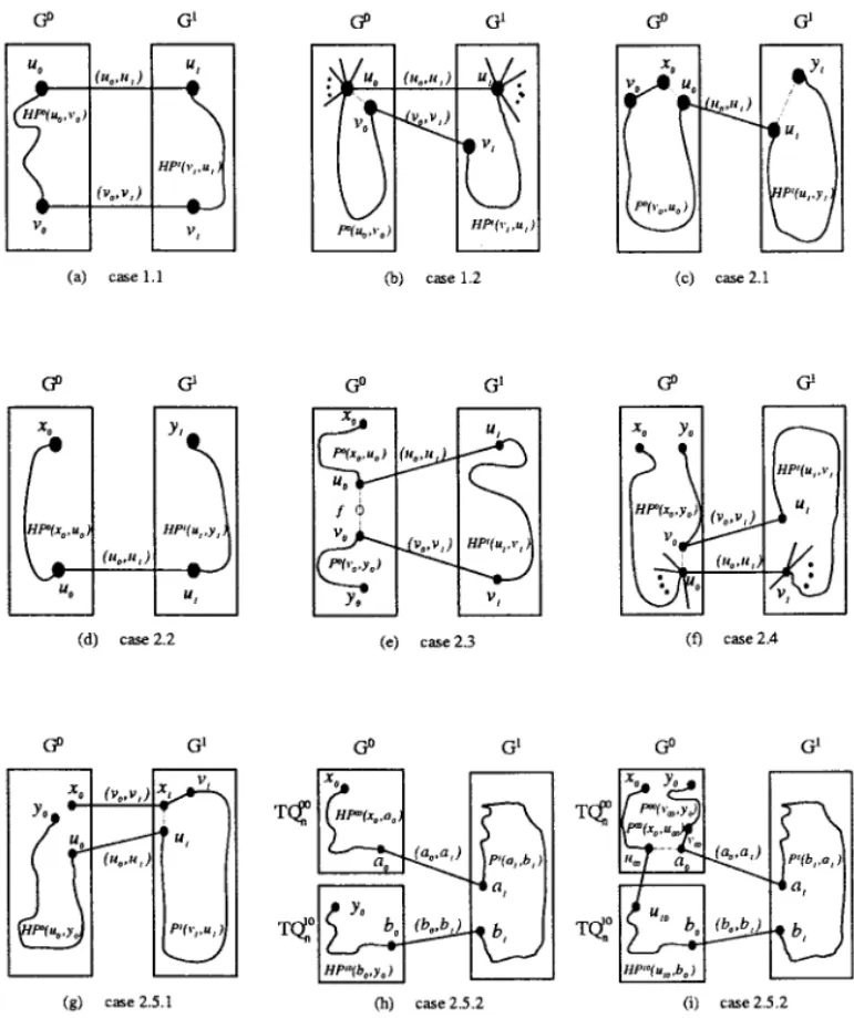
Case 1.1. fi=n for some i=0, 1. (All faults are on one side. See Fig. 5a.)
Without loss of generality, we assume that f0=n. Since G0=TQn× K2 is
(n − 1)-hamiltonian, there exists a hamiltonian path HP0(u
0, v0) joining some two
vertices u0, v0in G0− F. Since G1=TQn× K2 is hamiltonian connected, there exists
another hamiltonian path HP1(u
1, v1), where u1 and v1 are the matching nodes of
u0 and v0. Then, Ou0QHP0(u0, v0) Q v0Qv1QHP1(v1, u1) Q u1Qu0P forms a
hamiltonian cycle in (G0ÀMG1) − F.
Case 1.2. fi[n − 1 for both i=0, 1. (All faults are scattered over Ec, G0, or
G1. See Fig. 5b.)
Without loss of generality, we assume that f0\f1. Because f0+f1[n and
f1[f0[n − 1 for n \ 3, therefore f1[n − 2. Since G0 is (n − 1)-hamiltonian
and n − 1 \ f0, there exists a hamiltonian cycle HC0 in G0− F0. And G1 is
(n − 2)-hamiltonian connected and n − 2 \ f1, G1− F1 is a hamiltonian-connected
graph. Since 2n+1> 2n+1 for n \ 3, there exist two vertices u
0, v0 such that edge
(u0, v0) is on HC0 and u0, v0, u1, v1, (u0, u1), (v0, v1) ¨ F. Thus, there exists a
hamiltonian path HP1(v
1, u1). Let HC0=Ov0Qu0QP0(u0, v0) Q v0P. Then,
Ou0QP0(u0, v0) Q v0Qv1QHP1(v1, u1) Q u1Qu0P forms a hamiltonian cycle in
(G0À
MG1) − F.
Then, we prove that (G0À
MG1) is (n − 1)-hamiltonian connected. In other
words, we will prove that there exists a fault-free hamiltonian path between every pair of vertices xi and yj¥(V(G0ÀMG1) − F ), where F … (V(G0ÀMG1) 2
E(G0À
M G1)) and |F|=n − 1 for i, j ¥ {0, 1}. We prove this part by the following
cases.
Case 2.1. i ] j and fk=n − 1 for some k=0, 1. (xi and yj are on different
sides, and all faults are on one side. See Fig. 5c.)
Without loss of generality, we assume that i=0, j=1, and f0=n − 1. Since G0 is
(n − 1)-hamiltonian, there exists a hamiltonian cycle HC0 in G0− F. Let HC0=
Ox0Qu0QP0(u0, v0) Q v0Qx0P, in which u0, v0 are the vertices incident to x0and
P0(u
0, v0) is a path between u0, v0. Because G1is hamiltonian connected, there exists
a hamiltonian path between every pair of vertices of G1. If u
1]y1 where u1 is the
matching nodes of u0, then Ox0Qv0QP0(v0, u0) Q u0Qu1QHP1(u1, y1) Q y1P
forms a hamiltonian path joining x0 and y1 in (G0ÀM G1) − F. Otherwise, v1]y1
where v1 is in the matching nodes of v0, and thenOx0Qu0QP0(u0, v0) Q v0Qv1Q
HP1(v
Case 2.2. i ] j and both f0, f1[n − 2. (xi and yj are on different sides, and all
faults are scattered over Ec, G0, or G1. See Fig. 5d.)
Without loss of generality, we assume that i=0 and j=1. Because 2n+1\n+2
for n \ 3, there exist two vertices u0, u1¨(F 2 {x0, y1}) and (u0, u1) ¨ F. Since both
G0 and G1 are (n − 2)-hamiltonian connected, and n − 2 \ f
0 and n − 2 \ f1, the
graphs G0− F
0and G1− F1are hamiltonian connected. Thus there exist hamiltonian
paths HP0(x
0, u0) and HP1(u1, y1) in G0 and G1, respectively. Therefore,
Ox0QHP0(x0, u0) Q u0Qu1QHP1(u1, y1) Q y1P forms a hamiltonian path
joining x0and y1in (G0ÀM G1) − F.
Case 2.3. i=j and fi=n − 1. (xi, yj, and all faults are on the same side. See
Fig. 5e.)
Without loss of generality, we assume that i=j=0. Let w be a fault of F. Since
G0 is (n − 2)-hamiltonian connected, G0− (F − {w}) contains a hamiltonian path
HP0(x
0, y0). Thus G0− F contains two node-disjoint paths P0(x0, u0) and P0(v0, y0)
where P0(x
0, u0) 2 P0(v0, y0)=HP0(x0, y0) − {w}. Because G1 is (n −
2)-hamilto-nian connected and n − 2 \ 0, there exists a hamilto2)-hamilto-nian path HP1(u
1, v1) in G1.
Therefore, Ox0QPo(x0, u0) Q u0Qu1QHP1(u1, v1) Q v1Qv0QP0(v0, y0) Q y0P
forms a hamiltonian path of (G0À
MG1) − F.
Case 2.4. i=j and both f0, f1[n − 2. (xi and yj are on the same side, and all
faults are scattered over Ec, G0, or G1. See Fig. 5f.)
Without loss of generality, we may assume that i=j=0. Since G0 is
(n − 2)-hamiltonian connected and n − 2 \ f0, there exists a hamiltonian path
HP0(x
0, y0). Because 2n+1\2n for n \ 3, there exists an edge (u0, v0) on the path
HP0(x
0, y0) such that u1, v1, (u0, u1), and (v0, v1) are not in F. Since G1 is
(n − 2)-hamiltonian connected and n − 2 \ f1, there exists a hamiltonian path
HP1(u
1, v1) in G1. Thus, (HP0(x0, y0) 2 {(u0, u1), (v0, v1)} 2 HP1(u1, v1)) − {(u0, v0)}
forms a hamiltonian path joining x0and y0in (G0À
MG1) − F.
Case 2.5. i=j and fk=n − 1 for k ] i. (xi and yj are on the same side, but all
faults are on the other side.)
Without loss of generality, we may assume that i=j=0 and f1=n − 1. We will
prove this case by the following subcases.
Subcase 2.5.1. x1¨F or y1¨F, where x1 and y1 are the matching nodes of x0
and y0, respectively. Without loss of generality, we may assume that x1¨F. (See
Fig. 5g.)
Since G1 is (n − 1)-hamiltonian, there exists a hamiltonian cycle HC1=
Ox1Qu1QP1(u1, v1) Q v1Qx1P. Because G0 is (n − 2)-hamiltonian and n − 2 \ 1,
G0− {x
0} is a hamiltonian-connected graph. Let HP0(z0, y0) denote a hamiltonian
path joining z0 and y0in G0− {x0} for every node z0 in G0− {x0}. If u0]y0, where
u0 is the matching nodes of u1, then Ox0Qx1Qv1QP1(v1, u1) Q u1Qu0Q
HP0(u
0, y0) Q y0P forms a hamiltonian path in (G0ÀMG1) − F. Otherwise, v0]y0,
and thenOx0Qx1Qu1QP1(u1, v1) Q v1Qv0QHP0(v0, y0) Q y0P forms a
hamil-tonian path in (G0À
Subcase 2.5.2. x1¥F and y1¥F. The discussion of this case is a little
compli-cated. Since G1 is (n − 1)-hamiltonian and f
1=n − 1, there exists a hamiltonian
cycle HC1in G1− F
1. Moreover, there are two consecutive nodes a1and b1 on this
cycle HC1, such that their matching nodes a
0 and b0 are on different sides of
G0=TQ
n× K2, say a0¥TQ00n and b0¥TQ10n , where TQ00n and TQ10n are the two
sides of G0. Let HC1=Oa
1QP1(a1, b1) Q b1Qa1P.
Consider the case that x0and y0are on different sides of G0=TQn× K2. Without
loss of generality, we may assume that x0¥TQ00
n and y0¥TQ 10
n (See Fig. 5h.) Since
TQn is hamiltonian connected, there exist hamiltonian paths HP00(x0, a0) and
HP10( y 0, b0) in TQ 00 n and TQ 10 n, respectively. ThusOx0QHP00(x0, a0) Q a0Qa1Q P1(a
1, b1) Q b1Qb0QHP10(b0, y0) Q y0P forms a hamiltonian path joining x0and
y0in (G0ÀM G1) − F.
Next, consider that x0 and y0 are on the same side of G0=TQn× K2. Without
loss of generality, we may assume that x0, y0¥TQ00n. (See Fig. 5i.)
We need to define notations before further discussions. The graph G0=TQ n× K2
has two sides, denoted by TQ00
n and TQ10n. For each node u00 (u10, respectively) in
TQ00
n (TQ 10
n, respectively), its matching node with respect to the two sides TQ 00 n and
TQ10
n is denoted by u10 (u00, respectively).
Since TQn is (n − 3)-hamiltonian connected and n − 3 \ 0, there exists a hamilto-nian path HP00(x
0, y0)=Ox0QP00(x0, u00) Q u00Qa0Qv00QP00(v00, y0) Q y0P,
where u00 and v00 are the two adjacent nodes of a0 on this path. Let HP10(z 10, b0)
denote a hamiltonian path joining z10 and b0 in TQ10n. If u10]b0, where u10 is the
matching node of u00 with respect to the two sides TQ00
n and TQ 10 n, then
Ox0QP00(x0, u00) Q u00Qu10QHP10(u10, b0) Q b0Qb1QP1(b1, a1) Q a1Qa0Q
v00QP00(v00, y0) Q y0P forms a hamiltonian path joining x0 and y0 in
(G0À
MG1) − F. Otherwise, v10]b0 where v10 is the matching node of v00 with
respect to the two sides TQ00
n and TQ 10
n, and thenOx0QP00(x0, u00) Q u00Qa0Q
a1QP1(a1, b1) Q b1Qb0QHP10(b0, v10) Q v10Qv00QP00(v00, y0) Q y0P forms a
hamiltonian path joining x0and y0in (G0ÀMG1) − F. This completes the induction
proof. L
Now we are ready to prove our main theorem: Theorem 2.3. The twisted n-cube TQ
n is (n − 2)-hamiltonian and (n −
3)-hamil-tonian connected, for all odd integer n \ 3.
Proof. By Lemma 2.2, TQ3 is 1-hamiltonian and hamiltonian connected. And
TQn+2=(TQn× K2) ÀM(TQn× K2) for some perfect matching M. By Theorems
2.1 and 2.2, and by a simple induction, this theorem follows. L
It is obvious that the fault-tolerant hamiltonicity Hf(G) (the fault-tolerant
hamiltonian connectivity Ho
f(G), respectively) of a graph G is no greater than
d(G) − 2 (d(G) − 3, respectively), and TQn is a regular graph of degree n. From
Theorem 2.3 above, we have the following result. Corollary 2.1. H
f(TQn)=n − 2 and H
o
f(TQn)=n − 3, for all odd integer
3. CONCLUSIONS
In this paper, we consider a faulty twisted n-cube TQn with edge and/or node
faults. We prove that TQn remains hamiltonian (hamiltonian connected,
respec-tively), even if it has up to n − 2 (n − 3, respectively) edge and/or node faults. This result is optimum in the sense that the tolerant hamiltonicity (the fault-tolerant hamiltonian connectivity, respectively) of TQn is at most n − 2 (n − 3, respectively). As far as the hypercube network Qn is concerned, its vertex
fault-tolerant hamiltonicity is 0 and edge fault-fault-tolerant hamiltonicity is n − 2, for n \ 2. Recently, many topological properties of the twisted n-cube have been studied [1, 2, 6, 8, 9]. All these results indicate that the performance of TQn is better than that of the hypercube in many aspects. Therefore, the twisted n-cube is an attractive alter-native to the hypercube network.
As noted in this paper, we observe that the fault-tolerant hamiltonicity and the fault-tolerant hamiltonian connectivity are essential parameters of an interconnec-tion network [10]. It would be an interesting issue to study more on this subject.
REFERENCES
1. S. Abraham and K. Padmanabhan, The twisted cube topology for multiprocessors: A study in network asymmetry, J. Parallel Distrib. Comput. 13 (1991), 104–110.
2. E. Abuelrub and S. Bettayeb, Embedding of complete binary trees in twisted hypercubes, in ‘‘Proceedings of International Conference on Computer Applications in Design, Simulation, and Analysis,’’ pp. 1–4, 1993.
3. R. Aleliunas and A. L. Rosenberg, On embedding rectangular grids in square grids, IEEE Trans. Comput. 31 (1982), 907–913.
4. L. Bhuyan and D. P. Agrawal, Generalized hypercube and hyperbus structures for a computer network, IEEE Trans. Comput. 33 (1984), 323–333.
5. J. A. Bondy and U. S. R. Murty, ‘‘Graph Theory with Applications,’’ North-Holland, New York, 1980.
6. C. P. Chang, J. N. Wang, and L. H. Hsu, Topological properties of twisted cube, Inform. Sci. 113 (1999), 147–167.
7. K. Day and A. E. Ai-Ayyoub, Fault diameter of k-ary n-cube networks, IEEE Trans. Parallel Distrib. Systems 8 (1997), 903–907.
8. P. A. J. Hibers, M. R. J. Koopman, and J. L. A. van de Snepscheut, The twisted cube, in ‘‘Parallel Architectures and Languages Europe,’’ Lecture Notes in Computer Science, pp. 152–159, Springer-Verlag, Berlin/New York, 1987.
9. W. T. Huang, J. M. Tan, C. N. Hung, and L. H. Hsu, Token ring embedding in faulty twisted cubes, in ‘‘Proceeding of the 2nd Inter. Conf. Parallel Sys. PCS ’99,’’ pp. 1–10, 1999.
10. S. Y. Hsieh, G. H. Chen, and C. W. Ho, Fault-Free Hamiltonian ring embedding in faulty arrangement graphs, IEEE Trans. Parallel Distrib. Systems 10 (1999), 223–237.
11. F. T. Leighton, ‘‘Introduction to Parallel Algorithm and Architectures: Array, Tree, Hypercube,’’ Morgan Kaufmann, Los Altos, CA, 1992.
12. S. Latifi, S. Q. Zheng, and N. Bagherzadeh, Optimal ring embedding in hypercubes with faulty links, Proc. IEEE Symp. Fault-Tolerant Comput. 42 (1992), 178–184.
13. R. A. Rowley and B. Bose, Fault-tolerant ring embedding in de-Bruijn networks, IEEE Trans. Comp. 12 (1993), 1480–1486.
14. A. Sengupta, On ring embedding in hypercubes with faulty nodes and links, Infor. Process. Lett. 68 (1998), 207–214.
15. T. Y. Sung, C. Y. Lin, Y. C. Chuang, and L. H. Hsu, Fault tolerant token ring embedding in double loop networks, Inform. Process. Lett. 66 (1998), 201–207.
16. Y. C. Tseng, S. H. Chang, and J. P. Sheu, Fault-tolerant ring embedding in a Star graph with both link and node failures, IEEE Trans. Parallel. Distrib. Systems (1997), 1185–1195.