重力平衡機構對機械手臂動態表現與壽命的影響評估

(1)

國

立

交

通

大

學

機械工程學系

博士論文

重力平衡機構對機械手臂動態表現與壽命的影響評估

Evaluation of the Variation in Dynamic Performance and Service

Life of a Manipulator after being Gravity Balanced

研究生

程貴仁

指導教授

鄭璧瑩博士

(2)

重力平衡機構對機械手臂動態表現與壽命的影響評估

Evaluation of the Variation in Dynamic Performance and Service

Life of a Manipulator after being Gravity Balanced

研究生：程貴仁 Student：Cheng, Kuei-Jen 指導教授：鄭璧瑩博士 Advisor：Dr. Cheng, Pi-Ying

國立交通大學機械工程學系

博士論文

A Dissertation

Submitted to Department of Mechanical Engineering College of Engineering

National Chiao Tung University in partial Fulfillment of the Requirements

for the Degree of PhD

in

Mechanical Engineering July 2011

(3)

重力平衡機構對機械手臂動態表現與壽命的影響評估

研究生：程貴仁指導教授：鄭璧瑩博士國立交通大學機械工程學系摘要在工業界，機械手臂已被廣泛的應用在生產線上，以增進產能及降低成本。然而目前在工業界所常見的機械手臂有一共同的現象，即設計負載遠低於自重。此起因於機械手臂需具有相當剛性的結構，以避免因外加的負載而導致結構產生過大的應力變形而影響定位精度。然而機械手臂系統剛性的提升導致了自重的增加，自重的增加不但可能會降低該機械手臂動態的表現，也增加了機械手臂的能源消耗量。機械手臂的動態表現常使用加速度半徑來表示。加速度半徑係用以度量一機械手臂在某特定組成及姿態下的動態表現，而該動態表現可藉由該機械手臂的組成、姿態及致動器的輸出能力來求得。當一機械手臂的動態表現是由加速度半徑代表時，其意指該機械手臂夾爪在該組成及姿態下，於所有方向可達成的最大加速度。傳統上增進機械手臂動態表現的方法有下述兩種：1.增大所使用致動器的輸出；2.降低結構重量。然而增大所使用致動器的輸出意指需較多的能量輸入或（且）提升所使用致動器的輸出規格。輸出規格的提升往往導致較大的空間損耗與成本的投入或減少其減額比；而輸入較多能量不符合環保與成本節約的原則，且易導致減額比的下降而降低系統可能的壽命。在降低結構重量部分，一般需使用更高級的材料、較複雜的結構形狀或減少系統剛性的方式達成。然而使用更高級的材料、較複雜的

(4)

結構形狀往往導致成本的增加；而減少系統剛性將使該機械手臂負載變形增加而降低其定位精度。故，傳統上所習用增進動態表現的兩種方式不但會導致較大的成本或空間損耗，且易使原機械手臂之可用性下降。在大多數的應用上，致動器的輸出主要消耗在克服機械手臂原始重量，僅有少部分用以加速其所夾持的物件。有鑑於此，本研究探討當應用重力平衡原理-即使用外加機構來消除原機械手臂與外加機構的自重影響，增進能源使用效率與節省使用成本時可能產生的影響。由於外加機構能消雖除機械手臂的自重影響，但也改變了該機械手臂的原始構造，所以可能會影響該機械手臂的動態表現與壽命。為能解決此一問題，本研究利用操控性比來評估外加機構對機械手臂動態表現的影響，並利用加速度衰化率作為機械手臂動態表現受使用所產生的誤差而下降之評估標準，並進而評估該外加機構對原機械手臂的可能壽命之影響。本研究所提出的方法，可有效的評估該應用重力平衡的外加機構對機械手臂動態表現與可能壽命的影響，使得設計人員得以同時評估機械手臂在能源使用效率、功能表現與可能使用壽命間的關係，以選出最佳符合該使用環境的機械手臂設計。關鍵字：重力平衡；操控性比；加速度衰化率

(5)

Evaluation of the Variation in Dynamic Performance and

Service Life of a Manipulator after being Gravity Balanced

Student：Cheng, Kuei-Jen Advisors：Dr. Cheng, Pi-Ying

Department of Mechanical Engineering National Chiao Tung University

ABSTRACT

Manipulators have widely been utilized in industrial field to do assembly jobs in production lines. There are many different types of manipulators have been deployed for different applications, but most of them have a common characteristic, and that is the payload of a manipulator is much smaller than its self-weight. This is because a manipulator needs stiff structure to prevent from the excessive deformation resulted from the objects it holds to keep the positioning accuracy. However, the stiff structure results in the increase of the self-weigh and consumes considerable the output of the actuators of the manipulator. This not only increases the energy being consumed but also decreases the dynamic performance of the manipulator.

The dynamic performance of a manipulator is usually presented by acceleration radius. Acceleration radius is an index which is used to measure of the acceleration capacity of a manipulator with a certain configuration and at a specific posture. Dynamic performance will be influenced by the configuration, the posture, and the output capacity of the constituent joint actuators of the manipulator under discussion. When it is represented by acceleration radius, it means that the maximum acceleration which the end of a manipulator with certain configuration can achieve in all directions at that specific posture.

Conventionally, there are two approaches can be used to increase the dynamic performance of a manipulator, and they are: 1. raising the output

(6)

limits of the actuators it uses; 2. reducing the weight of the manipulator system. Raising the output limits of the actuators means that more energy needs to be exerted or/and the specification of the actuators needs to be promoted. However, raising the output limits of the actuators would result in cost increase, and exerting more energy will increase the cost and reduce the derating rate. Lowering derating rate usually results in the decline of the designed service life.

Reducing the weight of a manipulator system usually can be achieved by using better and stiffer materials or complicated but stiffer structures, or reducing the materials it uses. Using better materials and structure means the increase in the fabrication cost. Reducing the materials in use means the stiffness of the system decreases, and this will result in the deterioration in positioning accuracy which is caused by the increase of the compliance of the system. Based on what is stated above, these two conventional approaches used to promote the dynamic performance of a manipulator are not suitable to be implemented in real cases.

In most applications, the output of actuators of a manipulator spends on counterbalancing the gravitational force resulted from the stiff but heavy structure, not on accelerating the object it holds. To redeem this insufficiency, this study utilizes auxiliary mechanisms which is designed based on gravity balance theory to eliminate the influence of the self-weight of a manipulator and the mechanism. However, the auxiliary mechanism can eliminate the influence of self-weight but also changes the configuration of the original manipulator. This change may affect the dynamic performance and the service life of the manipulator. To cope with this issue, this study utilizes maneuverability ratio to evaluate the influence of an auxiliary mechanism on the dynamic performance of a manipulator after being equipped with that mechanism. Besides, this study also utilizes deterioration rate to investigate the deterioration in dynamic performance

(7)

of a manipulator with the errors resulted from the operation and evaluate the influence on the designed service life.

This study provides an effective methodology to evaluate the influence of a gravity balance mechanism on the dynamic performance and the designed service life of a manipulator. With the help of proposed methodology, designers of manipulators can not only have the ability to find out the relationship among the energy efficiency, performance, and designed service life of a manipulator but also have the capability to choose the best design to match the prescribed service conditions based on the results of evaluation.

(8)

誌謝感謝指導教授鄭璧瑩博士在這些年來的教導與協助，增進了學術研究相關的能力，並完成本論文。感謝張起明博士與左明健博士在本論文寫作期間所提供的協助，也感謝口試委員金大仁教授、張起明博士、鍾添淦博士與陳昭亮博士對本論文的建議與指教。感謝我的家人、親友在我求學期間所給予的支持與鼓勵，也感謝同師門的學弟們及所有給予我協助的人們。感謝主，在您的關愛與許可下，學業得以完成。感謝所有的一切。程貴仁 2011年7月11日于新竹交大

(9)

List of Tables

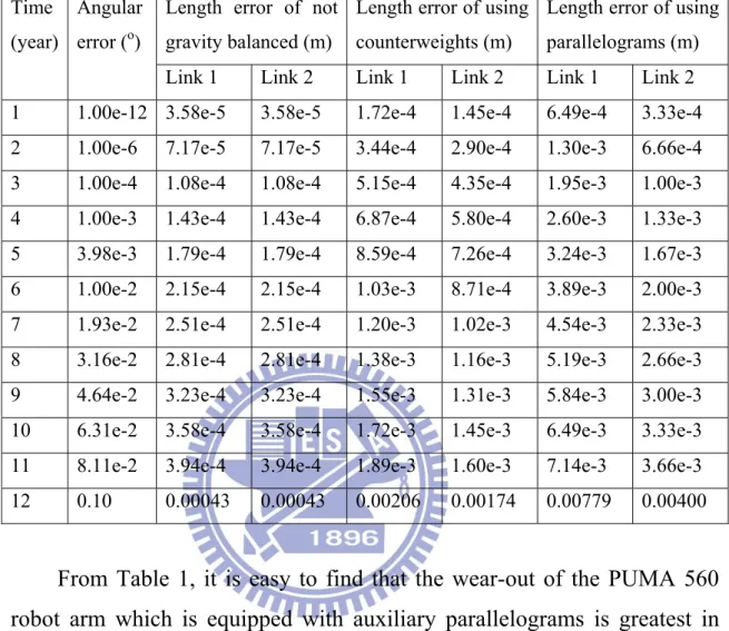
Page Table 1 Angular and length errors of a PUMA 560 robot arm without being gravity balanced, after being equipped with counterweights, and after being equipped with auxiliary parallelograms ... 48 Table 2 D-H parameters of the first three links of a PUMA 560 robot arm ... 50 Table 3 Inertial parameters of a PUMA 560 robot arm... 50 Table 4 Information of center of masses of the first three links and the

corresponding output limits of the joint actuators ... 50 Table 5 Parameters corresponding to the counterweights ... 52 Table 6 Parameters corresponding to the auxiliary parallelograms... 55

(12)

List of Figures

Page

Figure 1: The counterweight approach – a two-link example ... 11

Figure 2: The cam and spring approach – a single link example ... 13

Figure 3: The contour of the cam... 13

Figure 4: Two-link example of the orthosis approach... 15

Figure 5: Two-link example of the parallelogram approach ... 16

Figure 6: Definition of the acceleration radius with a 2 DOF example... 17

Figure 7. Diagrammatic definitions of D-H parameters ... 18

Figure 8: Diagrammatic definitions of modified D-H parameters ... 25

Figure 9: Failure block diagram of the original manipulator ... 42

Figure 10: Failure block diagram of a manipulator which is equipped with counterweights ... 43

Figure 11: Failure block diagram of a manipulator equipping with parallelograms... 44

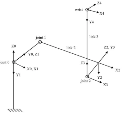
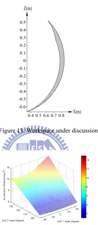
Figure 12: Zero position with attached frames of a PUMA 560 robot arm 50 Figure 13: Workspace under discussion ... 51

Figure 14: Dynamic Performance of a PUMA 560 robot arm without being equipped with any gravity balance mechanism ... 51

Figure 15: Skeleton drawing of a PUMA 560 robot arm which is equipped with the counterweights ... 53 Figure 16: (a) Dynamic performance of a PUMA 560 robot arm before and

(13)

Maneuverability ratio of a PUMA 560 robot arm equipped with the counterweights ... 53 Figure 17: Skeleton drawing of a PUMA 560 robot arm which is equipped

with the auxiliary parallelograms... 56 Figure 18: (a) Dynamic performance of a PUMA 560 robot arm before and

after being equipped with the auxiliary parallelograms (b) Maneuverability ratio of a PUMA 560 robot arm equipped with the auxiliary parallelograms... 56 Figure 19: The deterioration in dynamic performance of a PUMA 560 robot

arm after servicing for 1 year (a) without being gravity balanced (b) after being equipped with the counterweights (c) after being equipped with the auxiliary parallelograms... 57 Figure 20: The deterioration in dynamic performance of a PUMA 560 robot

arm after servicing for 2 years (a) without being gravity balanced (b) after being equipped with the counterweights (c) after being equipped with the auxiliary parallelograms ... 58 Figure 21: The deterioration in dynamic performance of a PUMA 560 robot

arm after servicing for 5 years (a) without being gravity balanced (b) after being equipped with the counterweights (c)

(14)

after being equipped with the auxiliary parallelograms ... 61 Figure 24: The deterioration in dynamic performance of a PUMA 560 robot

(15)

balanced (b) after being equipped with the counterweights (c) after being equipped with the auxiliary parallelograms ... 68 Figure 31: The run chart of the deterioration in the dynamic performance of

(16)

Glossary

m _：Mass

c _{：Distance between the center of mass of a link and its} corresponding joint

cm_{：Weight of counterweight}

l _{：Length between two ends of a link or distance between} two specified points of a link

wc ：Distance between the center of mass of counterweight and its corresponding joint

r _{：Effective radius of a cam}

k _{：Stiffness coefficient of a spring}

g _{：Gravitational acceleration}

 _{：Angle between two specified objects around z axis (if} applicable)

c

r ：Actual radius of a cam

 _{：Angle between effective and actual radiuses of a cam}

f _{：External force}

h _{：Vertical distance}

s _{：Length associates with an auxiliary parallelogram}

X _{：Position vector described in world space}

i

r ：Acceleration radius without the effect of errors

e

r _{：Acceleration radius with the effect of errors}

d _{：Distance between two consecutive frames along z axis}  _{：Angle between two consecutive frames around x axis} a _{：Distance between two consecutive frames along x axis}

A _{：D-H transformation matrix between two consecutive}

frames

T _：_{D-H transformation matrix between two non-consecutive}

frames

R _{：Rotation part of D-H transformation matrix} P _{：Translation part of D-H transformation matrix}

v _{：Linear velocity described in world space} w _{：Angular velocity described in world space} J _{：Jacobian matrix}

(17)

q _{：Position vector described in the joint space}

 _{：Force or torque vector proposed by actuators} ( , )

c q q ：Torque or force vector resulted from centrifugal and Coriolis forces

( )

g q ：Torque or force vector resulted from gravitational force

( )

M q _{：Inertia matrix}

L _{：Actuator output matrix} MR_{：Maneuverability ratio}

 _{：Angle between two consecutive frames around y axis} H _{：Wear depth}

S _{：Relative slide distance}

K _{：Wear coefficient} p _{：Contact pressure}

(18)

I. Introduction

This study investigates the variation in the dynamic performance and the designed service life of a manipulator after being equipped with a gravity balance mechanism. Service life means that a product can keep performing its designed functions without any unacceptable outcome. This study also proposes a methodology to evaluate the possible service life of a manipulator. Acceleration radius is usually utilized to be a measure of evaluating the dynamic performance of a manipulator with a certain configuration and at a specific posture, and it means that the maximum achievable acceleration in all directions at that posture. This study utilizes acceleration radius to evaluate the dynamic performance of a manipulator and uses maneuverability ratio to investigate and evaluate the variation in the dynamic performance of a manipulator before and after it is equipped with a gravity balance mechanism. Besides, deterioration rate is used in this study to evaluate the deterioration in dynamic performance of a manipulator resulted from the errors which are produced during the operation and to investigate how these errors influence the service life of a manipulator before and after being equipped with a gravity balance mechanism. In the following sections, the motivation and the goals of this study will be interpreted.

1.1 Motivation

In industrial field, many kinds of manipulators are designed to do the assembling job in the production line or perform some function in hazard environments. They indeed improve the productivity and quality of products and prevent humans getting injure from working environments. However, many of the manipulators used in industrial field have one common characteristic which is that the weight of the manipulator system itself is much greater than the payload at its end-effector. The stiff and

(19)

heavy structure is used to assure the stiffness of the manipulator is sufficient to counter the loading exerting on it to prevent excessive deformation which will deteriorate its positioning accuracy, especially when the manipulator is at a fully stretched posture. The stiff and heavy structure of a manipulator will consume considerable output energy of the constituent joint actuators to counterbalance the influence of self-weight even when this manipulator is in static working conditions. For many applications, manipulators spend most of their time on static or low-speed applications. However, these manipulators still need to spend considerable energy on counterbalancing their self-weight [1] even in these static or low-speed applications, and this will increase the operation cost.

To cope with this problem, the concept of gravity balance is proposed decades ago, and it successfully eliminates the influence of self-weight of a manipulator. For decades, gravity balance models and theories have been studied and investigated in a large volume of literature [2-22], such as the mathematical models of the auxiliary parallelogram approach [22]. In [5], it also emphasizes that after a manipulator has been gravity balanced, the energy efficiency of the manipulator shall become better, and the quantity of the energy can be saved by gravity balance mechanisms can be calculated by following the methodology provided in [1] and [10]. At the same time, many special designs have been developed and successfully satisfy the specific requirements of different applications [1, 23-31], such as an orthosis mechanism which can be used to assist the lower-limb disable patients to stand up from the sitting posture [33]. Meanwhile, the required actuator output which is used to perform a specific task before and after a manipulator is equipped with a gravity balance mechanism has been investigated in some studies [32]. However, as the author’s best knowledge, there is no other researcher discusses what the variation in dynamic performance is before and after a manipulator is equipped with a gravity

(20)

balance mechanism, and they all focus on how to eliminate the influence of the self-weight or the required actuator output used to perform a specific task after a gravity balance mechanism is applied. Because manipulators are not just designed for or dedicated to static or low-speed applications and definitely not just designed for a specific task, this will lead to insufficient conclusions. How the gravity balance mechanism influences the dynamic performance after a manipulator is equipped with it needs to be considered.

After a gravity balance mechanism equips to a manipulator, the configuration of a manipulator is changed, and the loading exerting on each constituent joint and the mass arrangement of the system change too. This means the wear-out of each joint and dynamic performance of the manipulator will change associatively. Besides, the equipped gravity balance mechanism may make the dynamic performance of the manipulator more sensitive to the deviation of the parameters of Denavit–Hartenberg transformation matrix (D-H parameters) and may decline the designed service life which is based on the dynamic performance after the manipulator is equipped with a gravity balance mechanism. Although the subject of investigating the designed service life of a product has been studied for more than 50 years, there is limited literature which discusses the designed service life of a manipulator based on its functional performance, and all of the literature only takes the positioning [34-39] or velocity [36] performance as the functional performance of the corresponding manipulator. As the author’s best knowledge, there is no other researcher discusses the designed service life of a manipulator including its dynamic performance which is represented by acceleration radius. This makes the study on the designed service life of manipulators insufficient.

(21)

variation in the dynamic performance and the designed service life of a manipulator after being equipped with a gravity balance mechanism.

1.2 Literature Review

The concept of gravity balance was proposed decades ago, and its function is to counterbalance the self-weight of a manipulator to reduce the loading on the constituent joint actuators of a manipulator and promote the energy efficiency in static or low-speed applications. General speaking, there are two approaches can be used to satisfy the requirement of gravity balance. The first one is using counterweights to counterbalance the gravitational force resulted from the self-weight [5,8,18,23], and the other is utilizing springs and auxiliary links which include wires and cams to keep the summation of the gravitational potential energy of the manipulator system and the elastic potential energy of the spring system constant [1,4,12-15,17,19-20,22,24,27-29,31,33]. Although there are still other approaches which are able to keep manipulators in gravity balance [6,21,25-26,30], such as full spring approach [21], they are rarely used in practice.

In [5], [8], and [18], they investigate how to apply counterweights to the parallel mechanisms to eliminate the self-weight influence. In [23], it studies the torque which is needed to each joint actuator of a PUMA 760 robot arm to perform the motion which follows a prescribed trajectory after the robot arm is gravity balanced by using the counterweights.

How to use cams and springs to eliminate self-weight is introduced in [24] and [31]. Using auxiliary links and springs to form the orthosis to eliminate the self-weight influence is interpreted in [13-14], [17], [19], [28-29], and [33]. In [1], [4], [12], [15], [20], [22], and [27], using auxiliary links and springs to form auxiliary parallelograms to eliminate the self-weight is demonstrated.

(22)

[6] and [30] introduce how to only use auxiliary links to fix the center of mass of the whole system to a inertial position to keep the potential energy of this system invariant to achieve gravity balance. In [21] and [26], only using springs to fully or partially eliminate the self-weight influence is explained. Using strings to hang the weight of each links to eliminate the self-weight influence is introduced in [25].

In [2], it introduces how to use counterweights or auxiliary links and springs to eliminate the self-weight influence of planar linkages. [3] includes the effect of deformation into the discussion of a 2 DOF gravity balanced mechanism. In [7], it compares the influence of different transmission structures on the performance of gravity balance. [9] and [10] introduce how to use counterweights or auxiliary links and springs to eliminate the self-weight influence on certain postures or in a region. The performance comparison of a mechanism after being gravity balanced by counterweights and springs on lifting a certain weight is introduced in [11]. The classification of gravity balanced industrial robots is interpreted in [16]. In [32], it compares the velocity performance of a manipulator after being gravity balanced by counterweights and springs along a prescribed path.

Acceleration radius was proposed to be the index of measuring the dynamic performance of a manipulator with a certain configuration and at a specific posture in the 80’s. In that period, the studying focus was on what the definition of dynamic performance would be and how to express it [40-42]. In the 90’s, the dynamic performance of a redundant manipulator was wildly investigated, and these studies focused on finding the better expression and calculation methodology [43-48]. After the millennium, the influence of velocity on the dynamic performance of a manipulator started to be investigated [49-52]. Recently, the study on this field started to investigate the influence of the fabrication and assembly errors on the dynamic performance of a manipulator [53]. These studies really do a great

(23)

contribution on researching the dynamic performance of a manipulator and greatly progress the development in robotics.

The service life of a product started to be systematically investigated by the U.S. military in the 50’s. For decades, much literature studied on this field had been proposed and promoted the quality of industrial products greatly. However, there are still few studies focus on the service life of a manipulator based on its functional performance until now [34-39]. All of these studies which investigate the service life of a manipulator only take the positioning or velocity performance as the functional performance of the manipulator, not including its dynamic performance.

1.3 Goal and Contribution

As the author’s best knowledge, there is no other researcher investigates the variation in dynamic performance of a manipulator after being equipped a gravity balance mechanism, and this leads their conclusions on the applicability of gravity balance mechanisms insufficient. To rectify this insufficiency, this study utilizes acceleration radius as the index to evaluate the dynamic performance before and after a gravity balance mechanism equips to a manipulator. For gaining the quantitative information about how a gravity balance mechanism influences the dynamic performance of a manipulator, this study utilizes maneuverability ratio to evaluate whether being equipped with gravity balance mechanisms would improve or degrade the dynamic performance of a manipulator.

Because manipulators used in industrial field are not just for static or low-speed applications, the studying on the designed service life of manipulators should not be limited to the scopes of positioning accuracy and velocity performance as the functional performance. The evaluation of the designed service life of a manipulator should include its dynamic performance to match practical applications. To rectify this insufficiency,

(24)

this study utilizes deterioration rate as the dynamic performance deterioration index to evaluate the deterioration of dynamic performance of a manipulator and uses this index to investigate the variation in the designed service life which is based on the dynamic performance before and after the manipulation is equipped with a gravity balance mechanism.

This study not only discusses the variation in the dynamic performance of a manipulator before and after being equipped with a gravity balance mechanism, but also is the first one which discusses the designed service life of a manipulator based on its dynamic performance. The methodology proposed in this study includes using maneuverability ratio to evaluate the variation in dynamic performance and introducing the configuration errors into the model of acceleration radius to conduct deterioration rate to verify whether the dynamic performance is still acceptable after certain time in service. With the help of what is proposed by this study, the variation in the dynamic performance and the designed service life based on the dynamic performance of a manipulator after being equipped with a gravity balance mechanism can be found out. This can not only help designers of manipulators verify whether installing a gravity balance mechanism to a manipulator is beneficial to the application but also help them to choose the best design based on the requirements of the application.

In order to systematically and comprehensively introduce the fundamentals, methodology, and the conclusions used or proposed in this study, this study is arranged as follows: In Chapter II, it reviews the fundamentals of gravity balance, acceleration radius, maneuverability ratio, and deterioration rate. Chapter III interprets how to conduct maneuverability ratio to evaluate the variation in the dynamic performance of a manipulator before and after being equipped with a certain gravity balance mechanism. The designed service life evaluation of a manipulator

(25)

before and after being equipped with a certain gravity balance mechanism is performed in Chapter IV. Chapter V takes a PUMA 560 robot arm as an example to interpret how to use the proposed methodology and how it works. In Chapter VI, some conclusions are proposed.

(26)

II. Fundamental Review

In this chapter, it introduces the fundamental theories and approaches used in this study. For systematically introducing these theories and approaches, this chapter is arranged as follows: in Section 2.1, it introduces the fundamentals of each principle category of gravity balance mechanisms. How to conduct the acceleration radius to measure the dynamic performance of a manipulator with a certain configuration at a specific posture is explained in Section 2.2. Section 2.3 introduces how to conduct maneuverability ratio to evaluate the variation in the dynamic performance of a manipulator before and after being equipped with a gravity balance mechanism. In Section 2.4, how to conduct deterioration rate which is used to evaluate the influence of errors which is resulted from fabrication or assembly processes on the dynamic performance of a manipulator is provided.

2.1 Gravity Balance

Gravity balance means that using a special developed approach eliminates the influence of the self-weight of a manipulator or mechanism. Generally speaking, there are two approaches which can be applied to a manipulator or a mechanism to satisfy the definition of gravity balance without consuming any extra energy. The first one is the counterweight approach, and the other is the auxiliary link and spring approach. In the following subsections, the fundamental of each approach will be introduced.

2.1.1 The Counterweight Approach

The counterweight approach utilizes a counterweight to place the center of mass of a link and its successive links and their corresponding counterweights to the corresponding joint. The sequence of applying counterweights to a manipulator is from its last link to its first link

(27)

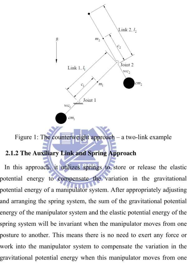
progressively. After applying a counterweight to the first link, the center of mass of the whole manipulator system locates at the joint which connects the base and the first link. Because the center of mass of the manipulator system is fixed to an inertial joint, the gravitational potential energy of the manipulator system will keep in constant from one posture to another. Since there is no change in the gravitational potential energy, it is no need to exert any force or work into the manipulator system to compensate the variation in its gravitational potential energy. For providing a clearer explanation of the concept and implementation of the counterweight approach, a two-link manipulator is taken as the example and shown in Figure 1. In the counterweight approach, the weight of each counterweight is unknown and needs to be calculated because it depends on the dimensions, configuration and weight arrangement of the manipulator. For this two-link example, the weights of each counterweight in use are shown in (1) and (2), respectively. For a general case, the weight of each counterweight can be calculated from (3) [33].

1 1 2 2 1 1 1 ( ) m c cm m l cm wc    (1) 2 2 2 2 m c cm wc  (2) 1 ( ) n i i i j j j i i i m c l cm m cm wc         (3)

Where n is the number of links; cm_i and cm_j are the weight of counterweight of link i and link j respectively; m_i is the weight of link i ; m_j is the weight of link j ; c_i is the distance between the center of mass of link i and joint i ; l_i is the length of link i ;

i

(28)

link i to joint i .

Figure 1: The counterweight approach – a two-link example

2.1.2 The Auxiliary Link and Spring Approach

In this approach, it utilizes springs to store or release the elastic potential energy to compensate the variation in the gravitational potential energy of a manipulator system. After appropriately adjusting and arranging the spring system, the sum of the gravitational potential energy of the manipulator system and the elastic potential energy of the spring system will be invariant when the manipulator moves from one posture to another. This means there is no need to exert any force or work into the manipulator system to compensate the variation in the gravitational potential energy when this manipulator moves from one posture to another. Generally speaking, the auxiliary link and spring approach includes three sub-approaches, and they are: the cam and the spring approach, the orthosis approach, and the auxiliary parallelogram approach. In the following subsections, the fundamental of each of the

(29)

three approaches will be introduced.

2.1.2.1 The Cam and Spring Approach

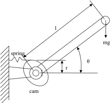
In the cam and spring approach, the contours of the cams are specialized according to the dimensions, configuration and weight arrangement of the manipulator they will be applied to. When in application, a spring will be dragged along with the contour of the corresponding cam to store or release its elastic potential energy to compensate the variation in gravitational potential energy of the corresponding link of the manipulator system. To explain this approach more clearly, a single link system is taken as the example and is shown in Figure 2. The contour of the cam of this example is depicted in Figure 3. When the diameter of the wire connecting the spring and the cam is negligible, the contour of the cam for this single link system can be conducted by following (4), (5), and (6) [24].

(sin cos ) 2 2 2 mgl r k



   (4) (5 3sin ) 8 mgl rc  _k 



(5) 1 1 tan [ (csc tan )] 2



_  _



_



₍₆₎

Where r is the effective radius of the cam; k is the stiffness

coefficient of the spring; mg is the effective gravitational force of the self-weight; l is the distance from the joint axis to the location of the

effective weight;



is the angle between the link and the horizontal

plane; c represents the real leave point of the wire to the cam; r is _c

the actual radius following the cam shape;



is the angle deviation

(30)

Figure 2: The cam and spring approach – a single link example

Figure 3: The contour of the cam

2.1.2.2 The Orthosis Approach

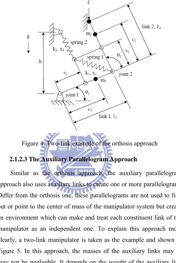
In the orthosis approach, it utilizes auxiliary links to create one or several parallelograms among the constituent links of a manipulator to identify or point to the center of mass of the manipulator system. Then a zero free length spring is used to connect the joint which identifies or points to the center of mass of the manipulator system to a certain inertial place. Then use other zero free length springs to connect each parallelogram to a certain place which depends on the dimensions, link number, configuration, and weight arrangement of the manipulator. In

dr dθ To spring r _r_c π/2-θ δ c r mg l θ cam spring

(31)

this approach, the length of auxiliary link and the stiffness coefficient are the parameters need to be conducted. Figure 4 shows a two-link example which can be used to lift up heavy weight and external force in the gravitational direction with relative small input force, and the

lengths of the auxiliary links (l₁ and s₁ s ) are expressed in (5) and ₂

(6) respectively, and the stiffness coefficients of the springs (k and ₁

2

k ) can be calculated by (7) and (8) respectively [33].

2 1 1 2 1 1 1 1 1 2 2 2 ( ) s m gc m gl fl l s l m gc fl       (5) 2 2

0s  , and l s must satisfy ₂ 0  s₁ l₁ (6)

1 2 2 2 1 2 1 1 ( ) ( ) s m gc fl k hs l s    (7) 2 2 2 2 2 m gc fl k hs   (8)

Where f is the external force exerted on the end point of link 2

in the gravitational direction; m and ₁ m are the masses of link 1 and ₂

link 2 respectively; c and ₁ c are the distance from the center of ₂

mass of link 1 to joint 1 and the distance from the center of mass of

link 2 to joint 2 respectively; l and ₁ l are the lengths of link 1 and ₂

link 2 respectively; h is the vertical distance from one end of spring 2

to the base;



₁ and



₂ are the angles from the base to link 1 and the

(32)

Figure 4: Two-link example of the orthosis approach

2.1.2.3 The Auxiliary Parallelogram Approach

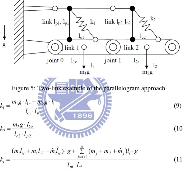
Similar as the orthosis approach, the auxiliary parallelogram approach also uses auxiliary links to create one or more parallelograms. Differ from the orthosis one, these parallelograms are not used to find out or point to the center of mass of the manipulator system but create an environment which can make and treat each constituent link of the manipulator as an independent one. To explain this approach more clearly, a two-link manipulator is taken as the example and shown in Figure 5. In this approach, the masses of the auxiliary links may or may not be negligible. It depends on the weight of the auxiliary link and how the accuracy of the result it needs. If the weight of the auxiliary link is relative small when it compares with the one of the corresponding link of the manipulator or the required accuracy is not too high, the weight of the auxiliary link can be neglected to simplify

(33)

the calculation and evaluation. When the masses of the auxiliary links are negligible in this example, the stiffness coefficients of the springs can be expressed as (9) and (10), respectively. When the masses of the auxiliary links are not negligible, the general form of calculating the stiffness coefficient of each spring can be expressed as (11) [20].

Figure 5: Two-link example of the parallelogram approach

1 1 2 1 1 1 1 c c p m g l m g l k l l      (9) 2 2 2 2 2 c c p m g l k l l    (10) ci pi n i j j j j i ic i ic i ic i i _l _l g l m m m g l m l m l m k            1 ) ˆ ( ) ˆ ˆ ( (11)

Where k is the stiffness coefficient of the spring i ; _i m and _i

j

m are the masses of link i and link j respectively; m and i m j are the masses of auxiliary link i and auxiliary link j which are

parallel to link i and link j respectively; mˆ and _i mˆ are the _j

masses of auxiliary link i and auxiliary link j which are parallel to

the gravitational direction respectively; l is the distance between _ic

(34)

along link i and between joint i and the center of mass of 1

auxiliary link i which is parallel to the gravitational direction; l_i is

the distance from the joint which connects one end of auxiliary link i

which is parallel to the gravitational direction and link i to joint i ; 1

pi

l is the height which is from the one end of spring i to the

connecting joint of link l and link i in the gravitational direction; _pi

ci

l is the distance which is along link i and between the one end of

spring i to the connecting joint of link l and link i . _pi

2.2 Acceleration Radius

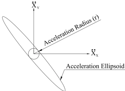
Acceleration radius is the index which is mostly used to measure the dynamic performance of a manipulator with a certain configuration at a specific posture under known output limits of the constituent joint actuators. Acceleration radius is defined as the maximum achievable acceleration in all directions of the end-effector of a manipulator at a specific posture. In Figure 6, it demonstrates a two degree of freedoms (DOF) example for providing a visual and clearer explanation of the definition of acceleration radius.

X

Acc

eler

atio

n R

adiu

s (r

)

Acceleration Ellipsoid

Y X

X

(35)

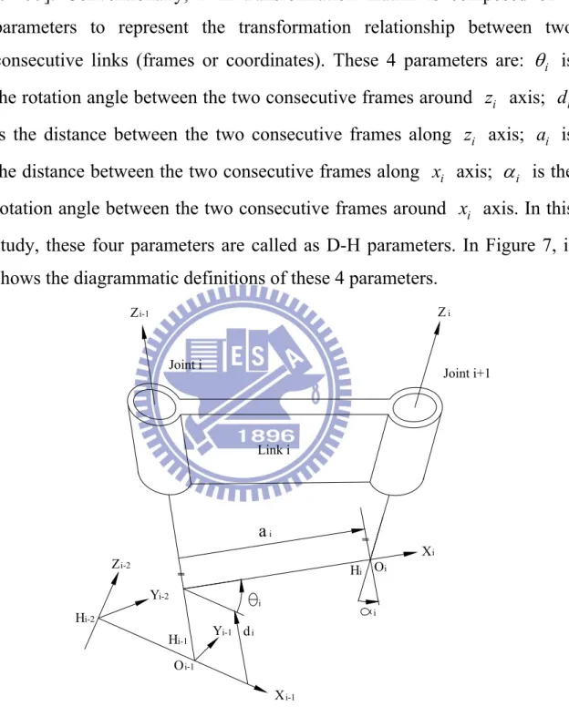
Before introducing acceleration radius, Denavit-Hartenberg transformation matrix (D-H transformation matrix) must be interpreted first [54-55]. Conventionally, D-H transformation matrix is composed of 4 parameters to represent the transformation relationship between two

consecutive links (frames or coordinates). These 4 parameters are:



_i is

the rotation angle between the two consecutive frames around z axis; _i d _i

is the distance between the two consecutive frames along z axis; _i a is _i

the distance between the two consecutive frames along x axis; _i



_i is the

rotation angle between the two consecutive frames around x axis. In this _i

study, these four parameters are called as D-H parameters. In Figure 7, it shows the diagrammatic definitions of these 4 parameters.

i Link i Joint i Joint i+1 Z Z Z X X H H d a i i i-1 i-1 i-2 i-2 i i-1 i i i i-1 O O Yi-2 i-1 Y i H

Figure 7. Diagrammatic definitions of D-H parameters

Based on the definitions of D-H parameters and their diagrammatic

explanation shown in Figure 7, D-H transformation matrix from link i

(36)

1 0 0 0 0 1 i i i i i i i i i i i i i i i i i i i C S C S S a C S C C C S a S A S C d                    _           (12)

Where i1A_i is the D-H transformation matrix from link i frame to

link 1i frame; S represents the sine function; C represents cosine

function.

When a manipulator is composed of n links, the D-H transformation matrix from the frame which locates at the end-effector to the base or

reference frame, T , can be expressed as (13). _n

1 1 0 1 n i n n n i i R P T  A      _{ } _   (13)

Where R is the rotation portion of _n T ; _n P is the translate portion _n

of T . _n

After introducing the total transformation matrix of a manipulator, how to conduct Jacobian matrix will be explained in the following discussion. Jacobian matrix is used to transform the constituent joint velocities of a manipulator in the joint space to the velocity of the end-effector in the world space. For a non-redundant manipulator, Jacobian matrix can be expressed as (14).

n n n n n n v x J q w    _{ }      (14)

Where n is the number of the constituent joints; v is the linear _n

velocity vector of the end-effector in the reference frame (world space); w _n

is the angular velocity vector of the end-effector in the world space; J_{n n}_

is the n n Jacobian matrix; _{q is the constituent joint velocity vector in}_n

(37)

1 1 1 1 ( ) n _i n i i n i i i v



z_  p z d_    _{ }    _ (15) 1 1 n n i i i w



z_     (16)

Where z_i_₁ is the z axis direction of the i frame which is 1 described in the reference frame and equivalent to the 3rd column vector of

1

i

R_ ; i1p_n is the position vector from end-effector to the origin of the i 1 frame and is also described in the reference frame;



 is the angular _i velocity of the thi revolute joint; d is the linear velocity of the _i

th

i prismatic joint.

From (15) and (16), the general form of Jacobian matrix can be expressed as (17). 1, ,...,2 n J _{ }J J J _{ (17)} Where 1 1 1 i i n i i z p J z           

 _{ is for a revolution joint, and}

1 0 i i z J _{  }    _{ is} for a prismatic joint.

After interpreting Jacobian matrix, the acceleration radius of a non-redundant manipulator will be introduced in the following. The first and second order differential kinematic equations of the end-effector of a non-redundant manipulator can be expressed as (18) and (19) respectively.

( ) n n n n x J _ q q_{ (18)} ( ) ( ) n n n n n n n x J q q J q q         (19)

Where q is the joint variable vector or angular position vector of the constituent joints described in the joint space; x is the position variable vector of the end-effector which is described in the reference frame.

(38)

( ) ( , ) ( )

M q q c q q g q



    (20)

Where



Rn is the vector of the constituent joint forces, torques, or

both; M q( )Rn n is the symmetric, positive definite inertial matrix;

( , ) n

c q q R is the vector of the forces, torques, or both resulted from

centrifugal and Coriolis forces; ( )g q Rn is the vector of the force, torque,

or both caused by external forces, torques, or both exerting on the manipulator.

From (20), the q can be expressed as (21).

1₍ ₎

q M 



 c g (21)

Take (21) into (19), x can be expressed as (22).

1 1 1 1 ( ) ( ) ( ) x JM c g Jq JM JM c Jq JM g



                  (22)

Where x is the acceleration vector of the end-effector which is

described in the reference frame; JM1



is the acceleration vector which

is contributed by the constituent joint actuators; (JM c Jq1   is the )

acceleration vector caused by the centrifugal and Coriolis forces;

1

(JM g ) is the acceleration vector resulted from the gravitational force

and external forces, torques, or both.

The output of an actuator used in industrial field usually has symmetric upper and lower limits. Thereof, the output range of each actuator used in a manipulator can be expressed as (23).

limit limit_, _{1 ~}

i i i i n



 

    (23)

After normalizing (23), the normalized output vector of the constituent

joint actuators, ˆ



, can be expressed as (24).

1

ˆ L



_ 



₍₂₄₎

(39)

element is equal to the output limit of the corresponding actuator and can be expressed as (25). limit 1 limit 0 0 0 0 0 0 _n L



            (25)

Because ˆ



is a normalized matrix, it has the characteristic which can

be expressed as (26).

ˆ ˆ 1T

 

 (26)

Through (22) and (24), x and



 can be expressed as (27) and (28)

respectively after appropriate arrangement.

1 _{ˆ (} 1 _{) (} 1 ₎ x JM L 



 JM c Jq    JM g   (27) 1 1 1 1 ˆ L MJ (x JM c Jq JM g)



_   _  _ _ _    (28)

Take (28) into (26), the equation of the acceleration ellipsoid can be conducted and expressed as (29).

1 1 1 1 1 1

(x JM c Jq JM g J M L L MJ_   _  )T T T T   (x JM c Jq JM g_   _  ) 1 ...(29)

After taking Q J M L L MJ T T T 1 1 and substitute it into (29), a

compact form of acceleration ellipsoid can be expressed as (30)

1 1 1 1

(x JM c Jq JM g Q x JM c Jq JM g     )T (     ) 1 (30) The value of acceleration radius is equal to the value of the radius of

the smallest inner tangent sphere of the acceleration ellipsoid which is centered in the origin of the reference frame. When a manipulator is at a standing posture, the acceleration radius will be equal to the reciprocal of the square root of the maximum eigenvalue of Q .

2.3 Maneuverability Ratio

After a manipulator is equipped with a gravity balance mechanism, its configuration changes, and its dynamic performance may vary and would

(40)

not be the same as the original one. To evaluate this variation, maneuverability ratio is developed and used to evaluate the variation in dynamic performance of a manipulator before and after being equipped with a gravity balance mechanism or a mechanism used for other purposes. Maneuverability ratio at a specific posture can be defined as (31), and this ratio in a specific workspace can be expressed as (32). With the help of this ratio, it is easy to quantitatively evaluate how much the dynamic performance of a manipulator improves or deteriorates after being equipped with a gravity balance mechanism or a mechanism used for other purposes.

g o P o r r MR r   (31)

Where MR_P is the maneuverability ratio at this specific posture; r_g

and r_o are the acceleration radiuses after and before being equipped with a

gravity balance mechanism respectively.

( ) w W w MR dw MR dw    (32)

Where MR is the maneuverability ratio in a prescribed workspace; _W

( )

w MR dw

 is the integral of the maneuverability ratio over the workspace;

wdw

 presents the workspace; MR is the maneuverability ratio at dw ;

dw presents the differential area of the workspace.

If MR_P or MR_W is positive, this means that equipping with this

gravity balance mechanism can improve the dynamic performance of the

manipulator and eliminate the influence of self-weight. If MR_P or MR_W

is negative, this means that being equipped with this gravity balance mechanism will sacrifice the dynamic performance of the manipulator though it eliminates the influence of self-weight. With the help of maneuverability ratio, designers of manipulators can get the information of how to adjust the setup of the controllers which will be used to perform the

(41)

trajectory planning automatically.

2.4 Deterioration Rate

Deterioration rate is an index of measuring the variation in the dynamic performance of a manipulator before and after including the influence of the errors which are resulted from the manufacturing, assembling, and operating processes. Deterioration rate is defined as the ratio of the deviation between the acceleration radius without and with the influence of the errors resulted from the manufacturing, assembling, and operating processes to the acceleration radius without these errors. The acceleration radius without the influence of these errors can be found out by using the processes provided in Section 2.2. However, finding out the acceleration radius with the influence of these errors which is due to the manufacturing, assembling, and operating processes is more complicated than finding the radius without the influence of these errors. How to conduct the acceleration radius with the influence of the errors resulted from the manufacturing, assembling, and operating processes will be explained in the following.

The first step of conducting the acceleration radius with the influence of the errors resulted from the manufacturing, assembling, and operating processes is to include the effect of these errors into the D-H parameters. The conventional D-H transformation matrix which has four D-H parameters is not sufficient to fully include the influence of these errors because it cannot include the angular error which is about the y axis. To cope with this insufficiency, an improved D-H transformation matrix which composes of five D-H parameters was proposed [56-58] and successfully includes all the effect of the errors resulted from the manufacturing, assembling, and operating processes into the transformation matrix. This kind of D-H transformation matrix which owns five D-H parameters is

(42)

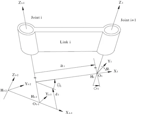
called modified D-H transformation matrix hereafter. In the modified D-H

transformation matrix, the extra parameter,



_i, is the rotation angle of the

two consecutive frames about y axis and is shown in Figure 8. The _i

modified D-H transformation matrix, i1A_i' can be conducted by

post-multiplying the conventional D-H transformation matrix, i1A_i , with

the rotation homogeneous matrix of



_i as shown in (33).

Figure 8: Diagrammatic definitions of modified D-H parameters

1 ' 1

0

1

0

1

0

1

i i i i i i i i i i i i i i i i i i i i i i i i i i i i i i i i i i i i i i i i i i i i i i i i i i

A

A A(y ,β )

Cθ

Sθ Cα

Sθ Sα

a Cθ

Cβ

Sβ

Sθ

Cθ Cα

Cθ Sα

a Sθ

Sα

Cα

d

Sβ

Cβ

Cθ Cβ

Sθ Sα Sβ

Sθ Cα Cθ Sβ

Sθ Sα Cβ

a Cθ

Sθ Cβ Cθ Sα Sβ

Cθ Cα

Sθ Sβ



_











_





































0

1

i i i i i i i i i i i

Cθ Sα Cβ

a Sθ

Cα Sβ

Sα

Cα Cβ

d







_





















(33)

(43)

Where A(y ,β ) is the rotation homogeneous matrix of _i _i



_i. When i



is equal to zero, (33) is fully equivalent to the conventional D-H

transformation matrix as shown in (12). In fact, the purpose of existence of i



is to include the rotation error about the y axis which is resulted from _i

the manufacturing, assembling, and operating processes. Because



_i is

used to introduce the influence of the angular error about the y axis, _i _i,

into the modified D-H transformation matrix,



_i itself has no intended

function and is always assigned to be zero in practical applications. When the errors resulted from the manufacturing, assembling, and operating processes exist in the modified D-H parameters, the corrective modified D-H transformation matrix which includes the influence of these errors can be expressed as the sum of the original modified D-H transformation matrix and the differential change matrix. The corrective modified D-H transformation matrix can be expressed as (34).

1 1 '

i C i

i i i

A A dA

 _  _ ₍₃₄₎

Where i1A_iC is the corrective modified D-H transformation matrix;

1 '

i i

A

 _{is the modified D-H transformation matrix with nominal modified}

D-H parameters; dA is the differential change matrix resulted from the _i

influence of the errors caused by the manufacturing, assembling, and

operating processes. Because



_i is always zero, then i1 'A_i  i1A_i ,

1 i

C



 , and S



_i  . To stress on the configuration errors have been 0

introduced into the D-H transformation matrix, i1 'A_i will still be used in

the following discussion. Assuming  ,



_i  , d_i  , a_i  , and



_i  are the



_i

errors of



_i, d , _i a , _i



_i, and



_i respectively. Because these errors are

always much smaller than the corresponding nominal modified D-H

(44)

without significantly losing the representativeness, and it can be expressed as (35). i i i i i i i i i i i i i i i i A A A A A dA d a d a                           (35) Set i i 1 i i A D_ A    _  , 1 i i d i i A D A d   _  , 1 i i a i i A D A a   _  , 1 i i i i A _D _A     _  , and 1 i i i i A D_ A      . Where 0 1 0 0 1 0 0 0 0 0 0 0 0 0 0 0 D_               ; 0 0 0 0 0 0 0 0 0 0 0 1 0 0 0 0 d D              ; 0 0 0 0 0 0 0 0 0 0 i i i i i i a i i S d S C d C D S C           _           ; 0 0 0 0 0 0 0 0 0 0 0 0 0 0 i i C S D_                ; 0 0 0 0 0 0 0 i i i i i i i i i i i i i i i i i i i i i i i i S C C a S S d C C S S C a C S d S C D C C S C a C                          _ _            From (35), 1 ( )i i i d i a i i i i dA  D_  D d  D a D_  D_  A (36) Set i 1 i i d i a i i i A D_ D d D a D_ D_

  _ _{ } _{ } _{ } _{ } _ _{, then the corrective}

modified D-H transformation matrix can be expressed as (37).

1 1 ' 1 1 ' ₍ 1 ₎ 1 ' i C i i i i i i i i i i i A A d A A  A A  _  _  _  _   ₍₃₇₎ Where

(45)

1 0 0 0 0 0 0 0 0 ( ) 0 ( ) 0 i i i i i i i i i i i i i i i i i i i i i i i i i i i i i i i i i i i i i i i i i i i i i i i i i i i i i i i i A S a C d S a C a S d C a S a C a d S C C a S S d C C S S C a C S d S C C C S C a C





 



 



 

  

 



 

  

 



  

 

         _ _ _ _{ } _                              0 0 0 0            

After conducting the corrected modified D-H transformation matrix, the total corrected modified D-H transformation matrix can be shown as (38). 1 1 1 ' 1 1( ) n n C i C i i n i i i i i T  A I



 A  A        (38)

Where n is the link number; I is a n n identity matrix.

Because the kinematic deviation resulted from the error items,



i1A_i, is relatively small, the influence of the second and higher order terms can be omitted without any significant influence on the result. In the following discussion, only the first order approximation of (38) will be utilized, and it can be presented as (39). 1 1 1 1 1 1 1 1 1 1 1 1 1 1 1 1 1 1 1 1 1 1 1 1 1 1 1 ( ) 0 1 ( ) [ ( )] ( ) 0 1 [ ( )] [ ( n n C i i i n n i i n i i i n i i C C n n n n n n i i i n n i i i n i i i i i i i i i n i i i n i i T T T A T I T AT T R P R R r R R P R r R P R r R P R p I R r R R I R                                                _ _ _ _ __ _             1 1 1 1 1 1 1 1 )] 1( ) 0 1 n n i i n i i i i i i i r R P i R r R P R p           _ __ _        (39)

重力平衡機構對機械手臂動態表現與壽命的影響評估

國

立

交

通

大

學

機械工程學系

博士論文

重力平衡機構對機械手臂動態表現與壽命的影響評估

Evaluation of the Variation in Dynamic Performance and Service

Life of a Manipulator after being Gravity Balanced

研 究 生

程貴仁

指導教授

鄭璧瑩 博士

重力平衡機構對機械手臂動態表現與壽命的影響評估

Evaluation of the Variation in Dynamic Performance and Service

Life of a Manipulator after being Gravity Balanced

重力平衡機構對機械手臂動態表現與壽命的影響評估

Evaluation of the Variation in Dynamic Performance and

Service Life of a Manipulator after being Gravity Balanced

Contents

List of Tables

List of Figures

Glossary





















X

Acc

eler

atio

n R

adiu

s (r

)

Acceleration Ellipsoid

X

























 













 











0

0

0

1

0

0

0

0

0

研究生

鄭璧瑩博士

_

_