Active noise cancellation in ducts using internal model-based control algorithms

IEEE TRANSACTIONS ON CONTROL SYSTEMS TECHNOLOGY, VOL. 4, NO. 2, MARCH 1996 163

Brief Papers

Active Noise Cancellation in Ducts Using Internal

Model-Based Control Algorithms

Jwu-Sheng

Hu

Abstract-A feedback control algorithm based on the internal model principle is proposed to solve the active noise control

(ANC) problem in ducts. Because of its infinite open-loop gain at selected frequencies, the controller is able, at the cancellation speaker position, to block noise transmission of these frequencies. In other words, the speaker acts like a totally reflective boundary. Stability analysis of the closed-loop system is performed using the Nyquist criterion. Experimental results confirm the theoretical analysis, showing an average noise level reduction of 30 to 40 dB at the target frequencies.

I. INTRODUCTION

CTIVE noise control (ANC) uses the principle of super-

A

imposing sound wave to cancel unwanted noises. This technique has received much attention during the last decade because of recent advances in electronics and microprocessors [8], [14]. Various studies on fan noise, exhaust noise, and motor noise [5], [15] show great potential in applying ANC to noise control problems. An effective ANC system requires an efficient control algorithm. Controller design based on modern control theories [3], [ 1 11 and signal processing techniques such as the FIR (finite impulse response) filter, the IIR (infinite impulse response) filter [5], [19], adaptive filters 1131, and ARMAX models [16] were studied. Due to the complex dynamics of sound, however, both the model-based and black- box types of controller design face the problems of closed-loop stability and performance evaluation.

This paper presents novel application of the internal model principle [7] to ANC. The internal model principle is a useful tool for disturbance rejection in feedback system design. One example is the so-called “repetitive controller” [9], [17]. In active noise control literature, a concept related to the internal model principle is the acoustical virtual earth [l], [18]. They found out that the pressure amplitude at the microphone can be greatly reduced if the open-loop gain is high. Moreover,

as started by Trinder and Nelson [18]: The acoustical virtual earth thus behaves like a perfectly reflecting open-ended duct termination situated by y;.

Here the y: is the location of the actuator. In other words, the noise will be totally reflected upstream if a pressure null

Manuscript received July 30, 1993; revised July 27, 1995. Recommended by Associate Editor, N. Yoshitani. This work was supported in part by the National Science Foundation of the United States under Grant MSS-9210756 and the National Science Council of the Republic of China under Grant The author is with the Department of Control Engineering, National Chao Publisher Item Identifier S 1063-6536(96)02075-0.

NSC84-22 12-E009-0 13.

Tung University, Hsiuchu, Taiwan, R.O.C.

is created at the actuator’s location. As will be shown later, an internal model-based controller, which has infinite open- loop gain at the target frequencies, can completely block noise transmission at those frequencies.

The stability of the closed-loop system is analyzed by using the Nyquist criterion. Since the internal model-based controller has unstable poles on the stability boundaries, the control gain must be carefully selected to avoid instability. Experimental results demonstrate the proposed controller’s effectiveness. An average reduction of 30 to 40 dB at target frequencies can be easily achieved.

As compared with feedforward control methods commonly used in ANC (for example, [4] and [6]), the internal model- based control law does not need to measure the noise signal, i.e., only a feedback sensor is required. Consequently, the acoustic feedback problem [6] encountered in a feedforward sensor is avoided. The proposed control law, however, can only deal with narrow-band noise since the signal model (rational transfer function) of a broad-band noise does not exist. Moreover, the success of this control law depends on an accurate internal model of the noise (e.g., frequency). For

applications such as the motor noise control, it is possible to synchronize the control law with the motor speed (e.g., using encoders to trigger the controller) to accurately pinpoint the noise frequency.

11. CLOSED-FORM TRANSFER FUNCTION

MODEL OF A DUCT

The one-dimensional dynamic equation of sound in a hard- walled duct can be described as in [ 2 ] and [121

where L , r , e , L G , p , and q are defined in the nomenclature section. The sound sources discussed in this paper are either force per unit mass or volume velocity source (such as a dipole). For a point dipole source located at

x

= a, (1)

becomes L2 dp2 &l

3

=

-

-

+

p L

-

{

- [.(t)]6(x - a ) } ( 2 ) 8x2 e2 at2

ax

at

with 1063-6536/96$05.00 0 1996 IEEE

Feedback Microphone

The duct's boundary conditions are described by the Noisesource

impedance function [2], (Pierce, 1981), i.e., at

x

= 0

x==a x=l

and at x = 1

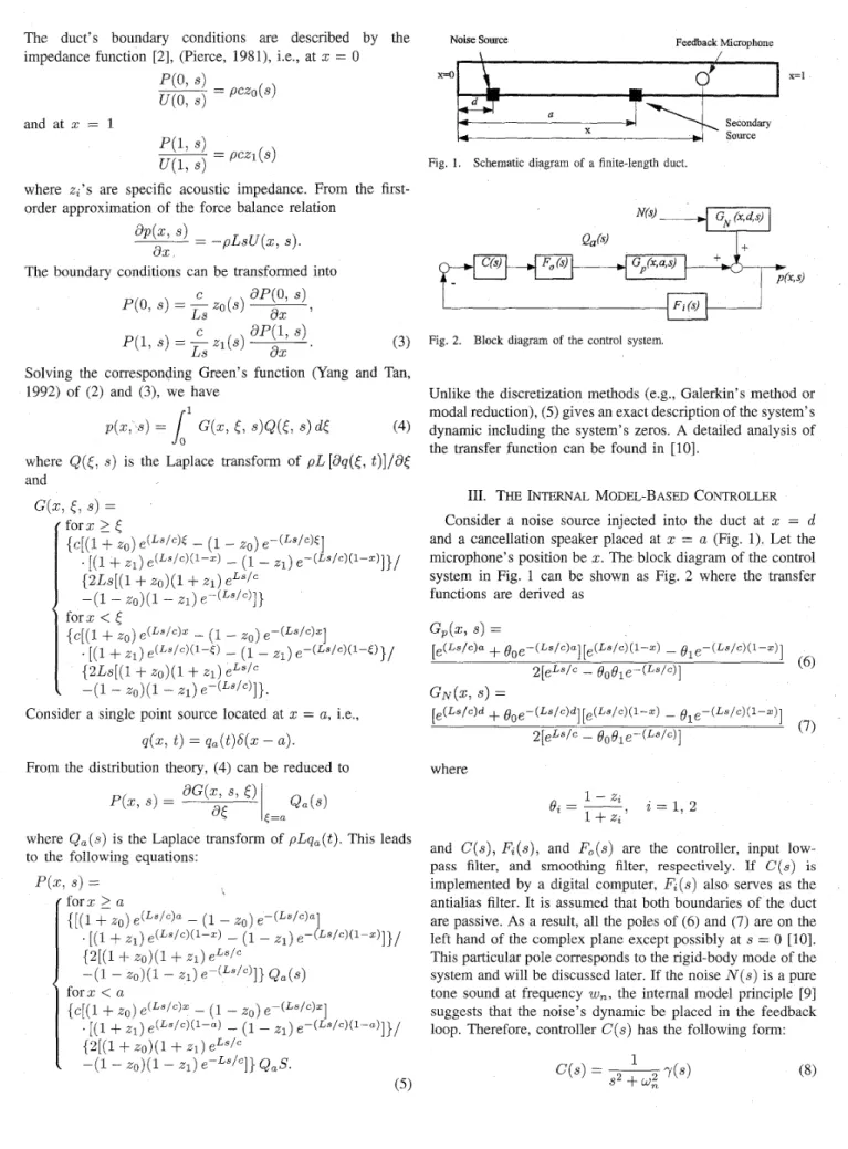
Fig. 1. Schematic diagram of a finite-length duct.

where zz's are specific acoustic impedance. From the first- order approximation of the force balance relation

d X

The boundary conditions can be transformed into

(3) Fig. 2. Block diagram of the control system.

C 5-1

P(1, s) = - z1(s) ~

Ls

ax

'

Unlike the discretization methods (e.g., Galerkin's method or modal reduction), (5) gives an exact description of the system's dynamic including the system's zeros. A detailed analysis of the transfer function can be found in [lo].

111. THE INTERNAL MODEL-BASED CONTROLLER

Consider a noise source injected into the duct at

x

= d

and a cancellation speaker placed at

x

=

a

(Fig. 1). Let the microphone's position be

x.

The block diagram of the control system in Fig. 1 can be shown as Fig. 2 where the transfer functions are derived as

From the distribution theory, (4) can be reduced to where

and C ( s ) , F,(s), and F,(s) are the controller, input low- pass filter, and smoothing filter, respectively. If C(s) is implemented by a digital computer, F,(s) also serves as the antialias filter. It is assumed that both boundaries of the duct are passive. As a result, all the poles of (6) and (7) are on the left hand of the complex plane except possibly at s = 0 [lo]. This particular pole corresponds to the rigid-body mode of the system and will be discussed later. If the noise N ( s ) is a pure tone sound at frequency w,, the internal model principle [9]

suggests that the noise's dynamic be placed in the feedback loop. Therefore, controller C ( s ) has the following form:

IEEE TRANSACTIONS ON CONTROL SYSTEMS TECHNOLOGY, VOL. 4, NO. 2, MARCH 1996 I65

where y(s) is an additional filter used to achieve closed-loop stability. To apply this controller, it is necessary that both

G,(z; s) and G N ( I C , s) do not vanish at s = j w n . This is usually achieved by carefully placing the microphone so

that the transmission zeros of both the noise and cancellation sources are not located at or near s = j w n [lo]. To analyze the effect of the internal model (8), first observe the following equality derived from (6) and (7):

The second terms on the right side of (12) and (13) represent the effect of noise without active cancellation while the first term depict the energy reflected due to cancellation.

To cancel noise with multiple tones, the controller (8) can be extended as

m

(14)

Pn n = l

GP(Y, j W ) G N ( Z , j w ) = G P ( ~ , j W ) G N ( Y , j w ) (9) The effect of applying (14) to the duct system is essentially the same as indicated in the previous analysis at a single frequency. It is also possible to write the controller in a serial form, i.e.,

where 1

2

2

a. The closed-loop response of the duct at is

m

The parallel structure of (14), however, allows a parallel hardware implementation of the controller. Besides, it is easy to determine the stability condition by using (14). This is the subject of the next section.

Since C ( j w n ) --f 00 (9), the pressure response at wn becomes

'(Y,

j w n > = -Gp(Y

,

j W n ) G N ( Z , j w n ) N ( j w n ) Gp(x, jw n >

Equation (1 1) means that by using an internal model-based controller, the noise at the segment of the duct, (1 _> y

2

a),

will be completely canceled. Hence, a pressure null (zero pressure) is created at the cancellation source. This result matches the concept of acoustic virtual earth raised by Trinder and Nelson [18]. In fact, the internal model creates a totally re- flective boundary so that the noise is driven upstream (between zero and a). The residual pressure response at y, a

2 2

0, is for a

2

. 1 ~

2

d

f o r d ? y 2 0

IV. STABILITY CONDITIONS

A. Continuous-Time Control System

Although the internal model-based controller (15) offers good performance in canceling noise at designated frequencies, it is, however, an unstable filter. Care must be exercised regarding the stability of the closed-loop system. The closed loop characteristic equation of the system is (10)

The Nyquist criterion makes it quite easy to determine the gains pi to guarantee stability. The following theorem states the condition:

Stability Condition I: All the roots of (16) are on the open left side of the complex plane if

and where G,"(Ic, s) = and G ~ ( z , s) = where

Equations (17b) and (17c) are closely related to the closed- loop roots on the imaginary axis. Notice that the set of gains which result in purely imaginary roots ( h j n ) satisfy

One of the important features of this condition is the way it allows the design of p z ’ s from experimental data, e.g., spec- trum. For a finite dimensional system (or lumped parameter system), the number of frequency points in set K (17c) is finite. An infinite dimensional system like the duct, however, may have an infinite number of points in K . Solving an infinite number of inequalities (17b) is not a practical approach. To resolve this problem, the conditions in (17) are replaced by sufficient ones. Since most of the cancellations occur in the low-frequency range, it is possible to find an upper bound of

R

=

Ru

such that w,

<

R,

for every n. Therefore, sufficient conditions to guarantee stability can be derived as follows.

Stability Condition 2: All the roots of (16) are on the open left-hand side of the complex plane if

forn = 1 N m

and

where

Only a finite number of inequalities has to be checked [(18b) and (18c)l.

B. Discrete-Time Control System

To implement noise cancellation using DSP’s (digital signal processors), it is necessary to formulate the problem in the digital domain. The discrete internal model-based controller can be written as m 1

--

I speaker

T--

microphone Fig. 3.

Time domain noise signal. (b) Noise spectrum.

Experimental setup (DSP: TMS320C30 Digital Signal Processor). (a)

TABLE I

DISCRETE-TIME TRANSFER FUNCTION OF THE DUCT (SAMPLING RATE = 10 IcHz)

POLE 0 0 0.1223 f j 0.1089 -0.0951 * j 0.4695 0.7358 + j 0.0592 0.7816 i j 0 . 1 7 6 7 0.8797

+

j 0.2753 0.8921 ij 0.4152 0.9380 + j 0.2972 0.9840 * j 0.0116 0.9900 i j 0.0575 0.9888

+

j 0.0984 0.9308 i j 0.3492 0.9067 k j 0.4086 0.9864 + j 0.1276 0.9760 fj 0.1921 0.9405 i j 0.3240 0.9822 + j 0.1604 0.9323 & j 0.2896 0.9620 + j 0.2561 0.9704 & j 0.2265 __p_ ZERO 5 5813 +J 15 7893 -3 8907 fj 1 0843 -1 2527 -0 5852 -0 3005 - 0 0 8 3 8 + ~ 0 0 1 1 8 0 0 0 4 1 ~ ~ 0 0 1 6 6 0 9072 i j 0 4042 0 9 8 2 8 + ~ 0 3 7 4 2 0 9013 + j 0 3532 0 9 4 3 7 + ~ 0 3 1 3 1 0 9 1 1 0 + ~ 0 3 0 0 2 10178 +J 0 2575 0 9235 +J 0 2380 0 9 7 6 1 k j 0 2 3 2 2 10418 f j 0 1336 0 9326 & J 0 1366 0 9825 +J 0 1473 0 9826 F J 0 0706 10262 10165

I

GAIN = 4.4082e-11

where T is the sampling time and 2-l is the back shift operator. Defining the digital plant as

Gd (2 - ) =

.{

F z

( 3 ) Gp (s)Fo (3))

IEEE TRANSACTIONS ON CONTROL SYSTEMS TECHNOLOGY, VOL. 4, NO. 2, MARCH 1996 167 I 0.5

g o

t

-0.5 1 0 1 0 IS 0 2 60 , 46.42dE

-

0

20

-

-

I

I

IO0 200 300 400 500 600 700 800 -40

w w

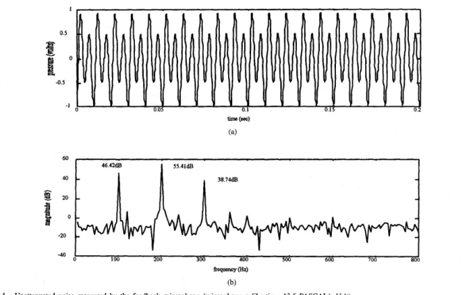
(Hz) (b)

Fig. 4. Unattenuated noise measured by the feedback microphone (microphone calibration: 13.5 PASCAL/mVolt).

teristic equation is Stability Condition 4: All the roots of (20) are inside the

unit circle if m 1

+

G ~ ( z - ' ) ~ ( z - ' ) P n ,unxIm {Gd(e-Jwn')r(e-JwnT)}

>

0 , n=l forn = 1

-

m ₍₂₂₄ = 0. (20)

One can derive stability conditions similar to the ones in the preceding section.

Stability Condition 3: All the roots of (20) are inside the unit circle if 1 - 2 COS ( j w , T ) z - l

+

2 - 2 Re {y(e-""T)Gd(e-3nT)e3'T}

>

-1 (22b)

1

Pn x

{

2

(wn

-

0 ) T sin ( W n

+

R ) T n=l 4 sin 2 2

,unxIm {Gd(e-""nT)y(e-3"-T)>

>

0 , and

(214 _{( w n - RuT sin ( w n}

₊

_Ru)T

forn = 1

-

m

1

(22c) 2 2

1

sin 4 m sup (Gd(e-3wT)y(e--3WT)I lbnl - w2nu Re

{

y (e--3 O T ) Gd ( e - J R T ) e J G T )

>

- 1 (2 1 b) where

R

E K = {wI Im { y ( e - ~ w T ) G d ( e - " T ) ( e " W T ) } = 0, CLn sin 2 2 w

< nu}.

where

a

E

K

=

{

Im {~(~-""T>G~(~-"T>.""T) = 0, V. SELECTION OF CONTROLLER PARAMETERS The closed-form transfer function formulation in Section

I1

explains the effect of an internal model-based control sys- tem. It is difficult, however, to obtain a closed-form transfer function in real practice. As a result, a reduced-order model is usually used for control system synthesis. While many 7r

w

5

T).

(21c)

By selecting an upper bound flu

<

n / T ,

the following sufficient condition can also be derived.

1 , o s 2z ?2

-

E o

E -0 5 I 0 05 0 1 0 I5 02 0 25 0 3 0 35 0 4 6o 40

5

-

I

12 51dB

z

20

I o

2

!

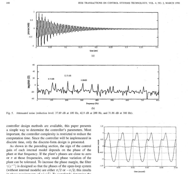
-20 -40 “cy (Hz) (b)

Fig. 5. Attenuated noise (reduction level. 37 89 dB at 100 Hz, 42 9 dB at 200 Hz, and 31 86 dB at 300 Hz).

controller design methods are available, this paper presents a simple way to determine the controller’s parameters. Most important, the controller complexity is restricted to reduce the computation time. Since the controller will be implemented in discrete time, only the discrete-form design is presented.

As shown in the preceding section, the sign of the control gain of each internal model depends on the phase of the plant at that frequency. If the plant’s phases are close to zero or 7r at those frequencies, only small phase variation of the

plant can be tolerated. To increase the phase margin, the filter ~ ( z - l ) is designed so that the phases of the open-loop system (without internal models) are either 7 r / 2 or -7r/2; this results in phase requirements of ~ ( 2 - l ) . To completely determine the parameters on ~ ( z - ’ ) , additional constraints are needed. One of the choices is to minimize the gain of ~ ( 2 - l ) (or H, norm) for better robustness properties. In other words, the following optimization problem can be formulated:

Cost function:

Constraints:

In this paper, the structure of g(2-l) was determined in advance to simplify computation. This point will be further illustrated in the experiment.

The control gain p,’s have a direct effect on the system’s performance. In active noise cancellation, a fast system re-

I I

-1 5

1

0 01 0 02 0 03 0 04 0 05 time (second)

Fig. 6 .

open end; solid line: active control off; dashed line: active control on). Sound pressure measured at a downstream position (1.2 m from the

sponse is important, especially when the noise characteristic (such as magnitude or phase) changes in time. To achieve this, the magnitude of closed-loop poles must be as small as

possible. Let the closed-loop poles be A,,

i

= 1 N N , where

N

is the order of the closed-loop system, and the following optimization problem is proposed:

Cost Function:

min max

p n i = l ~ N (24)

Constraints: (22a)-(22d).

Both the problems in (23) and (24) can be solved numeri- cally once a reduced-order plant is identified.

IEEE TRANS 169 70 60

-

SO

B

8

40

2

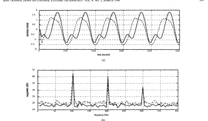
30 20 10

Fig. 7. Sound pressure active control on).

I I I I I I I

I

0 50 100 150 200 250 300 350 400

tlequency Wiz)

(b)

bignals measured at an upstream position (1 m from the cancellation speaker: solid line: active control off, dashed line:

VI. EXPERIMENTAL RESULTS

An experimental model was built to verify the proposed the- ory. Fig. 3 shows the schematic diagram of the experimental setup. The circular duct is made of PVC material 3.13 m long and 0.2 m in diameter. A TMS320C30 floating point digital signal processor hosted by a PC-AT is used to perform the computation

as

well as data acquisition. The antialias filter is a fourth-order Butterworth filter with a cutoff frequency of 3000 Hz. The cutoff frequency for the first mode of the duct is approximately 850 Hz. The cancellation speaker is placed 2.0 m and the microphone is placed 0.18 m from the open end of the duct. Another speaker is mounted at the other end to generate noise. Since our primary concern is low-frequency noise, the cutoff frequency of the smoothing filter (sixth-order Butterworth) is selected to be 500 Hz.

At a sampling rate of 10 kHz, the plants are identified as

F,(z-’)

= (0.1932-1

+

0 . 6 6 3 ~ - ~

+

0 . 2 4 5 ~ ~ ~

+

0 . 0 0 9 2 f 4 ) / (1

-

0.0542-1

+

0 . 2 1 ~ - ~ - 0 . 0 5 1 ~ - ~

+

0 . 0 0 6 2 ~ - ~ ) ,

+

2 8 3 . 8 2 ~ - ~

+

5 2 . 5 ~ - ~

+

0 . 9 0 3 ~ - ~ ) ] / [I - 5.852-1

+-

14.26z-’

-

1 8 . 5 6 ~ ~ ~

+

1 3 . 6 ~ ~ ~ - 5 . 3 2 ~ ~ ~

+

0.87.#]

FO(zp1)

= [2.12 x 10-ll(z-l

+

5 5 . 8 2 ~ ~ ~

+

2 8 9 . 6 8 ~ ~ ~

and the duct’s transfer function is shown in Table I. Three tonal noises are generated to demonstrate the con- trol system (100, 200, and 300 Hz). According to (19), the

controller can be written as

(1 - 1 . 9 9 6 L

+

2 - 2 C(z-1) = r(z-1) cL2 + 1 - 1.98422-1

+

2 - 2 + 1 - 1 . 9 6 4 6 ~ ~

+

x P 2 cL3

A simple choice of y(z-’) uses the FIR filter. The order of the filter is selected to be four. Solving (23), we obtain

r(2-l)

= 1 - 2.56182-1

+

1 . 4 5 0 4 ~ - ~

+

0 . 8 1 3 4 ~ - ~ - 0 . 7 6 0 1 ~ - ~

and the resulting maximum gain is 4.9661. To solve the control gain p,’s, the constraints in (23) are calculated by selecting R,

to be 600 Hz. One can choose a lower frequency to reduce the number of constraints, but it will result in a more conservative solution. The resulting control gains are computed as

pi =0.1030,

~2 =0.2624,

p3 =0.1309

and the maximum spectral radius of the closed-loop system

is 0.9981.

The noise generated by the speaker (measured at the feed- back microphone) is plotted in Fig. 4. Convergence of the error signal after ANC is plotted in Fig. 5(a). Although it takes about 4000 steps (0.4 s) to totally reduce the noise, laboratory experience shows that the response seems, to the

human ear, almost instant. From the spectrum [Figs. 4(b) and 5(b)], the controller is able to reduce the noise level by 38 dB at 100 Hz, 43 dB at 200 Hz, and 32 dB at 300 Hz. To verify that the noise is blocked at the cancellation speaker location, sound measurements are taken at other downstream points of

the duct. Fig. 6 depicts the pressure level of sound measured 1.2 m from the open end. Since the feedback microphone is not placed at this position, a small sound level still exists after the controller is turned on. The significant reduction in sound, however, justifies the theory presented in Section

111.

To verify the upstream reflection of noise, sound measurement is taken at an upstream position [Fig. 7(a)]. The increased sound energy level can be seen by comparing the spectrum shown in Fig. 7(b). An average increase of 6 dB reveals that the sound energy is approximately doubled.

VII. CONCLUSION

An internal model-based controller is proposed for active noise cancellation in ducts. It is shown that the controller can reduce the noise level by 30-40 dB at the downstream portions of the duct. Moreover, both theoretical and experimental results agree that the noise is driven to the upstream portion of the duct. While many ANC designs are based on feedfonvard types of algorithms, this paper shows that for noises with simple intemal models, it is possible to perform cancellation by a pure feedback configuration. Applications of the controller

to branched-duct systems as well as theoretical studies on convergent rates will be investigated in future research.

REFERENCES

[I] A. R. 0 . Curtis, P. A. Nelson, S. J. Elliott, and A. J. Bullmore, “Active suppression of acoustic resonance,” J. Acoust. Soc. Amer., vol. 81, pp. 624-631, 1987.

121 P. E. Doak, “Excitation, transmission and radiation of sound from sources in hard-walled ducts of finite length (1): The effect of duct

cross-section geometry and source distribution space-time pattern,” J. Sound Vibration, vol. 31, pp. 1-72, 1973.

[3] J. L. Dohner and R. Shoureshi, “Modal control of acoustic plahts,”

J. Vibration, Acoust., Stress, Reliability Design, vol. 11 1, pp. 326-330,

1989.

[4] L. J. Eriksson, M. C. Allie, and R. A. Greiner, “The selection and application of an IIR adaptive filter for use in active sound attenuation,”

IEEE Trans. Acoust., Speech, Signal Processing, vol. ASSP-33, no. 4, 1987.

[5] L. J. Eriksson, M. C. Allie, C. D. Bremigan, and J. A. Gilbert, “The use of active noise control for industrial fan noise,” in Proc. ASME Winter

Ann. Mtg., 1987.

[6] L. J. Eriksson, “Development of filtered-U algorithm for active noise control,” J. Acoust Soc. Amer., vol. 89, pp..257-265, 1991.

[7] B. A. Francis and W. M. Wonham, “The internal model principle for linear multivariable regulars,” AppZ. Math Optimization, vol. 2, pp. 170-194, 1975.

[8] R. T. Gorden and W. D. Vining, “Active noise control: A review of the field,” Amer. Ind. Hygiene Assoc. J., vol. 53, no. 11, Nov. 1992.

[9] S. Hara, Y. Yamamoto, T. Omata, and M. Nakano, “Repetitive control system: A new type of servo system for periodic exogenous signals,”

IEEE Trans. Automat. Contr., vol. AC-33, no. 7 , pp. 659-668, July 1988.

[lo] .J. Hu, “Active sound cancellation in finite-length ducts using closed form transfer function models,” ASME J. Dynamic Syst., Measurement, Contr., vol. 117, no. 2, pp. 143-154, 1995.

1111 A. J. Hull, C. J. liadcliffe, and C. R. MacCluer, “State estimation of the nonself-adjoint acoustic system,” ASME J. Dynamic Syst., Measure- ments, Contr., vol. 113-1, pp. 122-126, 1991.

[12] P. M. Morse and K. U. Ingard, Theoretical Acoustics. Princeton, NJ: Princeton Univ. Press, 1968.

[I31 K. Nagayasu and S. Susuki, “Application of active control to noise reduction by adaptive signal processing,” IEICE Trans. Fundamentals, vol. E75-A, no. 11, Nov. 1992.

[I41 P. A. Nelson and S. J. Elliott, “Active noise control: A tutorial review,”

IEICE Trans. Furuiamentals, vol. E75-A, no. 11, Nov. 1992. [lS] B. Sanito, “Electronic automobile muffler quiets the skeptics,” EE Times,

Oct. 1992.

[16] R. Shoureshi, N. Kubota, and G. Batta, “A modern control approach to active noise control,” in Proc. ASME Winter Ann. Mtg., Active Noise Vibration Contr., 1990, pp. 167-175.

[17] M. Tomizuka, T. C. Tsao, and K. K. Chew, “Discrete-time domain analysis and synthesis of repetitive controllers,” in Proc. Amer. Contr.

Cont. 1988, pp. 860-866.

[I81 M. C. J. Trinder and P. A. Nelson, “Active noise control in finite length ducts,’‘ J. Sound Vibration, vol. 89, pp. 95-105, 1983.

[I91 J. V. Warner, D. E. Water, and R. J. Bernhard, “Digital filter implemen- tation of local active noise control in a three dimensional enclosure,” ‘in